The motion of the Solar System and
the Michelson-Morley experiment

M. Consoli and E. Costanzo

Istituto Nazionale di Fisica Nucleare, Sezione di Catania
Dipartimento di Fisica e Astronomia dell’ Università di Catania
Via Santa Sofia 64, 95123 Catania, Italy

Abstract

Historically, the Michelson-Morley experiment has played a crucial role for abandoning the idea of a preferred reference frame, the ether, and for replacing Lorentzian Relativity with Einstein’s Special Relativity. However, our re-analysis of the Michelson-Morley original data, consistently with the point of view already expressed by other authors, shows that the experimental observations have been misinterpreted. Namely, the fringe shifts point to a non-zero observable Earth’s velocity $v_{\rm obs}=8.4\pm 0.5~{}{\rm km/s}$. Assuming the existence of a preferred reference frame, and using Lorentz transformations to extract the kinematical Earth’s velocity that corresponds to this $v_{\rm obs}$, we obtain a real velocity, in the plane of the interferometer, $v_{\rm earth}=201\pm 12~{}{\rm km/s}$. This value is in excellent agreement with Miller’s calculated value $v_{\rm earth}=203\pm 8$ km/s and suggests that the magnitude of the fringe shifts is determined by the typical velocity of the Solar System within our galaxy. This conclusion, which is also consistent with the results of all other classical experiments, leads to an alternative interpretation of the Michelson-Morley type of experiments. Contrary to the generally accepted ideas of last century, they provide experimental evidence for the existence of a preferred reference frame. This point of view is also consistent with the most recent data for the anisotropy of the two-way speed of light in the vacuum.

1. Introduction

The Michelson-Morley experiment [1] was designed to detect the relative motion of the Earth with respect to a preferred reference frame, the ether, by measuring the shifts of the fringes in an optical interferometer. These shifts, that should have been proportional to the square of the Earth’s velocity, were found to be much smaller than expected. Thus, that experiment was taken as an evidence that there is no ether and, as such, represented the essential ingredient for deciding between Lorentzian Relativity and Einstein’s Special Relativity.

However, according to some authors, the fringe shifts observed by Michelson and Morley, while certainly smaller than the classical prediction corresponding to the orbital velocity of the Earth, were not negligibly small. This point was clearly expressed by Hicks, see page 36 of Ref.[2] ”..the numerical data published in the Michelson-Morley paper, instead of giving a null result, show a distinct evidence of an effect of the kind to be expected” and also by Miller, see Fig.4 of Ref.[3]. In the latter case, Miller’s refined analysis of the half-period, second-harmonic effect observed in the original experiment, and in the subsequent ones by Morley and Miller [4], showed that all data were consistent with an effective, observable velocity lying in the range 7-10 km/s. For comparison, the Michelson-Morley experiment gave a value $v_{\rm obs}\sim 8.8$ km/s for the noon observations and a value $v_{\rm obs}\sim 8.0$ km/s for the evening observations.

Due to the importance of the issue, we have decided to re-analyze the original data obtained by Michelson and Morley and re-calculate the values of $v_{\rm obs}$ for their experiment. Our findings completely confirm Miller’s indication of an observable velocity $v_{\rm obs}\sim 8.4$ km/s in their data.

In addition assuming, as in the pre-relativistic physics, the existence of a preferred reference frame, but using Lorentz transformations to connect with the Earth’s reference frame, it turns out that this $v_{\rm obs}$ corresponds to a real Earth’s velocity, in the plane of the interferometer, $v_{\rm earth}\sim 201\pm 12$ km/s. This value, which is remarkably consistent with Miller’s kinematically calculated value $v_{\rm earth}\sim 203\pm 8$ km/s [3], suggests that the magnitude of the fringe shifts is determined by the typical velocity of the Solar System within our galaxy (and not, for instance, by its velocity $v_{\rm earth}\sim 336$ km/s with respect to the centroid of the Local Group).

We emphasize that the use of Lorentz transformations is absolutely crucial. In fact, in this case, differently from the classical predictions, the fringe shifts measured with an interferometer filled with a dielectric medium of refractive index ${\cal N}_{\rm medium}$ are proportional to the Fresnel’s drag coefficient $1-1/{\cal N}^{2}_{\rm medium}$. For this reason, a large ‘kinematical’ velocity $\sim 200$ km/s is seen, in an in-air-operating optical system, as a small ‘observable’ velocity $\sim 8.4$ km/s. At the same time, without using Lorentz transformation, there was no hope to understand why, for the same value of $v_{\rm earth}$, the effective $v_{\rm obs}$ had to be $\sim 3$ km/s for the Illingworth experiment (performed in an apparatus filled with helium) or $\sim 1$ km/s for the Joos experiment (performed in an evacuated housing).

2. The Michelson-Morley data

We have analyzed the original data obtained by Michelson and Morley in each of the six different sessions of their experiment. No form of inter-session averaging has been attempted. As discovered by Miller, in fact, inter-session averaging of the raw data may be misleading. For instance, in the Morley-Miller data [4], the morning and evening observations each were indicating an effective velocity of about 7.5 km/s (see Fig.11 of Ref.[3]). This indication was completely lost with the wrong averaging procedure adopted in Ref.[4]. The same point of view has been advocated by Munera in his recent re-analysis of the classical experiments [5].

To obtain the fringe shifts of each session we have followed the well defined procedure adopted in the classical experiments as described in Miller’s paper [3]. Namely, starting from the seventeen entries, say $E(i)$, reported in the Michelson-Morley Table [1], one was first correcting the data for the difference $E(1)-E(17)$ between the 1st entry and the 17th entry obtained after a complete rotation of the apparatus. Therefore, assuming the linearity of the correction effect, one was adding 15/16 of the correction to the 16th entry, 14/16 to the 15th entry and so on, thus obtaining a set of 16 corrected entries

$$E_{\rm corr}(i)={{i-1}\over{16}}(E(1)-E(17))+E(i)$$ (1)

Finally, the fringe shift is defined from the differences between each of the corrected entries $E_{\rm corr}(i)$ and their average value $\langle E_{\rm corr}\rangle$ as

$${{\Delta\lambda(i)}\over{\lambda}}=E_{\rm corr}(i)-\langle E_{\rm corr}\rangle$$ (2)

These final data for each session are shown in Table 1.

Following the above procedure, the fringe shifts are given as a periodic function (with vanishing mean) in the range $0\leq\theta\leq 2\pi$ with $\theta={{i-1}\over{16}}2\pi$. Therefore, they can be reproduced in a Fourier expansion

$${{\Delta\lambda(\theta)}\over{\lambda}}=\sum_{n}~{}\bar{A}_{n}\cos(n\theta+\phi_{n})$$ (3)

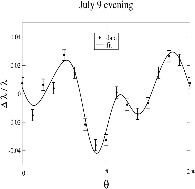
Figure 1: We show a typical fit Eq. (3) to the Michelson-Morley data shown in Table 1.

In this way, one can extract the amplitude $\bar{A}_{2}$ of the second-harmonic component which is the relevant one to determine the observable velocity. Following Miller’s indications, we have included terms up to $n=5$, although the results for $\bar{A}_{2}$ are practically unchanged if one excludes from the fit the terms with $n=4$ and $n=5$. The typical fit to the data is illustrated in Fig.1 while we report in Table 2 the values of $\bar{A}_{2}$ for each session.

The Fourier analysis allows to determine the azimuth of the ether-drift effect, from the phase $\phi_{2}$ of the second-harmonic component, and an observable velocity from the value of its amplitude. To this end, we have used the basic relation of the experiment

$$2\bar{A}_{2}={{2D}\over{\lambda}}~{}{{v^{2}_{\rm obs}}\over{c^{2}}}$$ (4)

where $D$ is the length of each arm of the interferometer.

Notice that, as emphasized by Shankland et al. (see page 178 of Ref.[6]), it is the quantity $2\bar{A}_{2}$, and not $\bar{A}_{2}$ itself, that should be compared with the maximal displacement obtained for rotations of the apparatus through $90^{o}$ in its optical plane (see also Eqs.(23) and (24) below). Notice also that the quantity $2\bar{A}_{2}$ is denoted by $d$ in Miller’s paper (see page 227 of Ref.[3]).

Therefore, for the Michelson-Morley apparatus where ${{D}\over{\lambda}}\sim 2\cdot 10^{7}$ [1], it becomes convenient to normalize the experimental values of $\bar{A}_{2}$ to the classical prediction for an Earth’s velocity of 30 km/s

$${{D}\over{\lambda}}~{}{{(30{\rm km/s})^{2}}\over{c^{2}}}\sim 0.2$$ (5)

and we obtain

$$v_{\rm obs}\sim 30~{}\sqrt{{\bar{A}_{2}}\over{0.2}}~{}~{}{\rm km/s}$$ (6)

Now, by inspection of Table 1, we find that the average value of $\bar{A}_{2}$ from the noon sessions, $\bar{A}_{2}=0.017\pm 0.003$, indicates a velocity $v_{\rm obs}=8.7\pm 0.8$ km/s and the average value from the evening sessions, $\bar{A}_{2}=0.014\pm 0.003$, indicates a velocity $v_{\rm obs}=8.0\pm 0.8$ km/s. Since the two determinations are well consistent with each other, we conclude that the Michelson-Morley experiment provides an ${\bar{A}}_{2}$ which is $\sim 1/13$ of the classical expectation and an observable velocity

$$v_{\rm obs}=8.4\pm 0.5~{}{\rm km/s}$$ (7)

in excellent agreement with Miller’s estimate.

Notice that this value is also in excellent agreement with the results obtained by Miller himself at Mt. Wilson. Differently from the original Michelson-Morley experiment, Miller’s data were taken over the entire day and in four epochs of the year. However, after the critical re-analysis of Shankland et al. [6], it turns out that the average daily determinations of $\bar{A}_{2}$ for the four epochs were statistically consistent (see page 170 of Ref.[6]). Therefore, one can take the average of the four daily determinations, $\bar{A}_{2}=0.044\pm 0.005$, and compare with the equivalent form of Eq.(5) for the Miller’s interferometer ${{D}\over{\lambda}}~{}{{(30{\rm km/s})^{2}}\over{c^{2}}}\sim 0.56$. Again, the observed $\bar{A}_{2}$ is just $\sim 1/13$ of the classical expectation for an Earth’s velocity of 30 km/s and the effective $v_{\rm obs}$ is exactly the same as in Eq.(7).

3. Miller’s 1932 cosmic solution

The problem with Miller’s analysis was to reconcile such low observable values of the Earth’s velocity with those obtained from the daily variations of the azimuth ( i.e. $\phi_{2}$) and magnitude (i.e. $\bar{A}_{2}$) of the ether-drift effect. In this way, on the base of the theory exposed by Nassau and Morse [7], Miller could obtain two determinations of the apex of the Earth’s motion for any given epoch of the year. These consist in two pairs of values $(\alpha,\delta)$ where $\alpha$ denotes the right ascension and $\delta$ the declination. The pair of values obtained from the variation of the azimuth, say $(\alpha$-Az,$\delta$-Az), and that obtained from the variation of the magnitude, say $(\alpha$-Mag,$\delta$-Mag), were found in good agreement with each other (see Fig.23 of Ref.[3]). Therefore, it makes sense to average the two determinations in a single value, say $(\langle\alpha\rangle,\langle\delta\rangle)$, for each of the four epochs of the year of his observations. These four average values lie, to a very good approximation, on the Earth’s ‘aberration orbit’, the centre of which is the apex of the cosmic component of the Earth’s motion. Subtracting out from each $(\langle\alpha\rangle,\langle\delta\rangle)$ the known effects of the Earth’s orbital motion, Miller could finally restrict kinematically the cosmic component of the Earth’s velocity in the range 200-215 km/s (see page 233 of Ref.[3]) with the conclusion that ”…a velocity $v_{\rm earth}\sim 208~{}{\rm km/s}$ for the cosmic component, gives the closest grouping of the four independently determined locations of the cosmic apex”. The direction of the apex thus determined points toward the midst of the Great Magellanic Cloud $20^{o}$ south of Canopus, the second brightest star in the heavens.

At the same time, due to the particular magnitude and direction of the cosmic component, Miller’s predictions for the total Earth’s velocity in the plane of the interferometer had very similar values (see Table V of Ref.[3]), say

$$v_{\rm earth}\sim 203\pm 8~{}{\rm km/s}$$ (8)

Therefore, after Miller’s observations, the situation with the ether-drift experiments could be summarized as follows (see page 236 of Ref.[3]). On one hand, ”the observed displacement of the interference fringes, for some unexplained reason, corresponds to only a fraction of the velocity of the Earth in space”. On the other hand, the theoretical solution of the Earth’s cosmic motion involves only the relative values of the ether-drift effect and ”..does not require a knowledge of the cause of the reduction in the apparent velocity nor of the amount of this reduction”. A check of this is that, after inserting the final parameters of the cosmic component in the Nassau-Morse expressions, ”..the calculated curves fit the observations remarkably well, considering the nature of the experiment” (see Figs. 26 and 27 of Ref.[3]).

In spite of this beautiful agreement, the unexplained large discrepancy between the typical values of $v_{\rm obs}$, as given in Eq.(7), and the typical calculated values of $v_{\rm earth}$, as given in Eq.(8), has been representing a very serious objection to the consistency of Miller’s analysis.

4. The role of Lorentz transformations

It has been recently pointed out, however, by Cahill and Kitto [8] that an effective reduction of the Earth’s velocity, from a large ‘kinematical’ value $v_{\rm earth}={\cal O}(10^{2})$ km/s down to a small ‘observable’ value $v_{\rm obs}={\cal O}(1)$ km/s, can be understood by taking into account the effects of the Lorentz contraction and of the refractive index ${\cal N}_{\rm medium}$ of the dielectric medium used in the interferometer.

In this way, the observations become consistent [8] with values of the Earth’s velocity that are comparable to $v_{\rm earth}\sim 365$ km/s as extracted by fitting the COBE data for the cosmic background radiation [9]. The point is that the fringe shifts are proportional to ${{v^{2}_{\rm earth}}\over{c^{2}}}(1-{{1}\over{{\cal N}^{2}_{\rm medium}}})$ rather than to ${{v^{2}_{\rm earth}}\over{c^{2}}}$ itself. For the air, where ${\cal N}_{\rm air}\sim 1.00029$, assuming a value $v_{\rm earth}\sim 365$ km/s, one would expect fringe shifts governed by an effective velocity $v_{\rm obs}\sim 8.8$ km/s consistently with our value Eq.(7).

This would also explain why the experiments of Illingworth [10] (performed in an apparatus filled with helium where ${\cal N}_{\rm helium}\sim 1.000036$) and Joos [11] (performed in the vacuum where ${\cal N}_{\rm vacuum}\sim 1.00000..$) were showing smaller fringe shifts and, therefore, lower effective velocities.

In Ref.[12] the argument has been completely reformulated by using Lorentz transformations (see also Ref.[13]). As a matter of fact, in this case there is a non-trivial difference of a factor $\sqrt{3}$. When properly taken into account, the Earth’s velocity extracted from the absolute magnitude of the fringe shifts is not $v_{\rm earth}\sim 365$ km/s but $v_{\rm earth}\sim 201$ km/s thus making Miller’s prediction Eq.(8) completely consistent with Eq.(7). For the convenience of the reader, we shall report in the following the essential steps.

The key point is that Lorentz transformations preserve the value of the speed of light in the vacuum $c=2.9979..10^{10}$ cm/s but do not preserve its value

$$u\equiv{{c}\over{\cal{N}_{\rm medium}}}$$ (9)

in a medium. In this case, due to a refractive index ${\cal N}_{\rm medium}>1$, one has to account for the effects of a non-vanishing Fresnel’s drag coefficient

$$k_{\rm medium}=1-{{1}\over{{\cal N}^{2}_{\rm medium}}}\ll 1$$ (10)

Therefore, if light would be seen to propagate isotropically with velocity Eq.(9) in one (‘preferred’) reference frame $\Sigma$, it will not be seen to propagate isotropically in any other frame $S^{\prime}$ that is in relative motion with respect to $\Sigma$.

Now, this is precisely the basic issue: determining experimentally, and to a high degree of accuracy, whether light propagates isotropically for an observer $S^{\prime}$ placed on the Earth. For instance within the air, where the relevant value is ${\cal N}_{\rm air}=1.00029..$, the isotropical value ${{c}\over{\cal{N}_{\rm air}}}$ is usually determined directly by measuring the two-way speed of light along various directions. In this way, isotropy can be established at the level $\sim 10^{-7}$. If we require, however, a higher level of accuracy, say $10^{-9}$, the only way to test isotropy is to perform a Michelson-Morley type of experiment and look for fringe shifts upon rotation of the interferometer.

Therefore, if one finds experimentally fringe shifts (and thus some non-zero anisotropy) it becomes natural to explore the possibility that this effect is due to the Earth’s motion with respect to a preferred frame $\Sigma\neq S^{\prime}$. Assuming this scenario, the degree of anisotropy for $S^{\prime}$ can easily be determined by using Lorentz transformations. By denoting ${\bf{v}}$ the velocity of $S^{\prime}$ with respect to $\Sigma$ one finds ($\gamma=1/\sqrt{1-{{{\bf{v}}^{2}}\over{c^{2}}}}$)

$${\bf{u}}^{\prime}={{{\bf{u}}-\gamma{\bf{v}}+{\bf{v}}(\gamma-1){{{\bf{v}}\cdot{\bf{u}}}\over{v^{2}}}}\over{\gamma(1-{{{\bf{v}}\cdot{\bf{u}}}\over{c^{2}}})}}$$ (11)

where $v=|{\bf{v}}|$. By keeping terms up to second order in $v/u$, denoting by $\theta$ the angle between ${\bf{v}}$ and ${\bf{u}}$ and defining $u^{\prime}(\theta)=|{\bf{u^{\prime}}}|$, we obtain

$${{u^{\prime}(\theta)}\over{u}}=1-\alpha{{v}\over{u}}-\beta{{v^{2}}\over{u^{2}}}$$ (12)

where

$$\alpha=(1-{{1}\over{{\cal N}^{2}_{\rm medium}}})\cos\theta+{\cal O}(({\cal N}^{2}_{\rm medium}-1)^{2})$$ (13)

$$\beta=(1-{{1}\over{{\cal N}^{2}_{\rm medium}}})P_{2}(\cos\theta)+{\cal O}(({\cal N}^{2}_{\rm medium}-1)^{2})$$ (14)

with $P_{2}(\cos\theta)={{1}\over{2}}(3\cos^{2}\theta-1)$.

Finally, the two-way speed of light is

$${{\bar{u}^{\prime}(\theta)}\over{u}}={{1}\over{u}}~{}{{2u^{\prime}(\theta)u^{\prime}(\pi+\theta)}\over{u^{\prime}(\theta)+u^{\prime}(\pi+\theta)}}=1-{{v^{2}}\over{c^{2}}}(A+B\sin^{2}\theta)$$ (15)

where

$$A={\cal N}^{2}_{\rm medium}-1+{\cal O}(({\cal N}^{2}_{\rm medium}-1)^{2})$$ (16)

and

$$B=-{{3}\over{2}}({\cal N}^{2}_{\rm medium}-1)+{\cal O}(({\cal N}^{2}_{\rm medium}-1)^{2})$$ (17)

To address the theory of the Michelson-Morley interferometer we shall consider two light beams, say 1 and 2, that for simplicity are chosen perpendicular in $\Sigma$ where they propagate along the $x$ and $y$ axis with velocities $u_{x}(1)=u_{y}(2)=u={{c}\over{{\cal N}_{\rm medium}}}$. Let us also assume that the velocity $v$ of $S^{\prime}$ is along the $x$ axis.

Let us now define $L^{\prime}_{P}$ and $L^{\prime}_{Q}$ to be the lengths of two optical paths, say P and Q, as measured in the $S^{\prime}$ frame. For instance, they can represent the lengths of the arms of an interferometer which is at rest in the $S^{\prime}$ frame. In the first experimental set-up, the arm of length $L^{\prime}_{P}$ is taken along the direction of motion associated with the beam 1 while the arm of length $L^{\prime}_{Q}$ lies along the direction of the beam 2.

In this way, the interference pattern, between the light beam coming out of the optical path P and that coming out of the optical path Q, can easily be obtained from the relevant delay time. By using the equivalent form of the Robertson-Mansouri-Sexl parametrization [14, 15] for the two-way speed of light defined above in Eq.(15), this is given by

$$\Delta T^{\prime}(0)={{2L^{\prime}_{P}}\over{\bar{u^{\prime}}(0)}}-{{2L^{\prime}_{Q}}\over{\bar{u^{\prime}}(\pi/2)}}$$ (18)

On the other hand, if the beam 2 were to propagate along the optical path P and the beam 1 along Q, one would obtain a different delay time, namely

$${(\Delta T^{\prime})}_{\rm rot}={{2L^{\prime}_{P}}\over{\bar{u^{\prime}}(\pi/2)}}-{{2L^{\prime}_{Q}}\over{\bar{u^{\prime}}(0)}}$$ (19)

Therefore, by rotating the apparatus and using Eqs.(16) and (17), one obtains fringe shifts proportional to

$$\Delta T^{\prime}(0)-(\Delta T^{\prime})_{\rm rot}\sim(-2B){{(L^{\prime}_{P}+L^{\prime}_{Q})}\over{u}}{{v^{2}}\over{u^{2}}}$$ (20)

or

$$\Delta T^{\prime}(0)-(\Delta T^{\prime})_{\rm rot}\sim{{3(L^{\prime}_{P}+L^{\prime}_{Q})}\over{u}}k_{\rm medium}{{v^{2}}\over{u^{2}}}$$ (21)

(neglecting ${\cal O}(\kappa^{2}_{\rm medium})$ terms). This coincides with the pre-relativistic expression provided one replaces $v$ with an effective observable velocity

$$v_{\rm obs}=v\sqrt{k_{\rm medium}}\sqrt{3}$$ (22)

Finally, for the Michelson-Morley experiment, where $L^{\prime}_{P}=L^{\prime}_{Q}=D$, and for an ether wind along the $x$ axis, the prediction for the fringe shifts at a given angle $\theta$ has the particularly simple form

$${{\Delta\lambda(\theta)}\over{\lambda}}={{u\Delta T^{\prime}(\theta)}\over{\lambda}}={{u}\over{\lambda}}({{2D}\over{\bar{u^{\prime}}(\theta)}}-{{2D}\over{\bar{u^{\prime}}(\pi/2+\theta)}})={{2D}\over{\lambda}}{{v^{2}}\over{c^{2}}}(-B)\cos(2\theta)$$ (23)

that corresponds to a pure second-harmonic effect. At the same time, it becomes clear the remark by Shankland et al. (see page 178 of Ref.[6]) that its amplitude

$$\bar{A}_{2}\equiv{{2D}\over{\lambda}}{{v^{2}}\over{c^{2}}}(-B)={{D}\over{\lambda}}{{v^{2}_{\rm obs}}\over{c^{2}}}$$ (24)

is just one-half of the corresponding quantity entering Eq.(20).

5. Interpretation of the Michelson-Morley observations

Now, if upon operation of the interferometer there are fringe shifts and if their magnitude, observed with different dielectric media and within the experimental errors, points consistently to a unique value of the Earth’s velocity, there is experimental evidence for the existence of a preferred frame $\Sigma\neq S^{\prime}$. In practice, to ${\cal O}({{v^{2}_{\rm earth}}\over{c^{2}}})$, this can be decided by re-analyzing [8] the experiments in terms of the effective parameter $\epsilon={{v^{2}_{\rm earth}}\over{u^{2}}}k_{\rm medium}$. The conclusion of Cahill and Kitto [8] is that the classical experiments are consistent with the value $v_{\rm earth}\sim 365$ km/s obtained from the COBE data.

However, in our expression Eq.(22) determining the fringe shifts there is a difference of a factor $\sqrt{3}$ with respect to their result $v_{\rm obs}=v\sqrt{k_{\rm medium}}$. Therefore, using Eqs.(22) and (7), for ${\cal N}_{\rm air}\sim 1.00029$, the relevant Earth’s velocity (in the plane of the interferometer) is not $v_{\rm earth}\sim 365$ km/s but rather

$$v_{\rm earth}\sim 201\pm 12~{}{\rm km/s}$$ (25)

This value, obtained from the magnitude of the fringe shifts, is in excellent agreement with the value Eq.(8) calculated kinematically by Miller. Therefore, from this excellent agreement, we deduce that the observed fringe shifts are determined by the typical velocity of the Solar System within our galaxy and not, for instance, by its velocity relatively to the centroid of the Local Group. In the latter case, one would get higher values such as $v_{\rm earth}\sim 336$ km/sec, see Ref.[16].

Notice that such ambiguity, say $v_{\rm earth}\sim 200,300,365,...$ km/s, on the actual value of the Earth’s velocity determining the fringe shifts, can only be resolved experimentally in view of the many theoretical uncertainties in the operative definition of the preferred frame where light propagates isotropically. At this stage, we believe, one should just concentrate on the internal consistency of the various frameworks. In this sense, the analysis presented in this paper shows that internal consistency is extremely high in Miller’s 1932 solution.

We are aware that our conclusion goes against the widely spread belief that Miller’s results were only due to statistical fluctuation and/or local temperature conditions (see the Abstract of Ref.[6]). However, within the paper the same authors of Ref.[6] say that ”…there can be little doubt that statistical fluctuations alone cannot account for the periodic fringe shifts observed by Miller” (see page 171 of Ref.[6]). In fact, although ”…there is obviously considerable scatter in the data at each azimuth position,…the average values…show a marked second harmonic effect” (see page 171 of Ref.[6]). In any case, interpreting the observed effects on the base of the local temperature conditions cannot be the whole story since ”…we must admit that a direct and general quantitative correlation between amplitude and phase of the observed second harmonic on the one hand and the thermal conditions in the observation hut on the other hand could not be established” (see page 175 of Ref.[6]). This rather unsatisfactory explanation of the observed effects should be compared with the previously mentioned excellent agreement that was instead obtained by Miller once the final parameters for the Earth’s velocity were plugged in the theoretical predictions (see Figs.26 and 27 of Ref.[3]).

The most surprising thing, however, is that Shankland et al. did not realize that Miller’s average value $\bar{A}_{2}=0.044\pm 0.005$, obtained after their own critical re-analysis of his observations, gives precisely the same $v_{\rm obs}$ Eq.(7) obtained from the Miller’s re-analysis of the Michelson-Morley experiment. Conceivably, their emphasis on the role of the temperature effects in Miller’s data would have been turned down whenever they had realized the perfect identity between two determinations obtained in completely different experimental conditions.

6. Comparison with other classical experiments

On the other hand, additional information on the validity of Miller’s results can also be obtained by other means, for instance comparing with the experiment performed by Michelson, Pease and Pearson [17]. These other authors in 1929, using their own interferometer, again at Mt. Wilson, declared that their ”precautions taken to eliminate effects of temperature and flexure disturbances were effective”. Therefore, their statement that the fringe shift, as derived from ”..the displacements observed at maximum and minimum at sidereal times..”, was definitely smaller than ”…one-fifteenth of that expected on the supposition of an effect due to a motion of the Solar System of three hundred kilometres per second”, can be taken as an indirect confirmation of Miller’s results. Indeed, although the ”one-fifteenth” was actually a ”one-fiftieth” (see pag.240 of Ref.[3]), their fringe shifts were certainly non negligible. This is easily understood since, for an in-air-operating interferometer, the fringe shift $(\Delta\lambda)_{\rm class}(300)$, expected on the base of classical physics for an Earth’s velocity of 300 km/s, is about 500 times bigger than the corresponding relativistic one

$$(\Delta\lambda)_{\rm rel}(300)\equiv 3k_{\rm air}~{}(\Delta\lambda)_{\rm class}(300)$$ (26)

computed using Lorentz transformations (compare with Eqs.(21) and (22) for $k_{\rm air}\sim{\cal N}^{2}_{\rm air}-1\sim 0.00058$). Therefore, the Michelson-Pease-Pearson upper bound

$$(\Delta\lambda)_{\rm obs}<0.02~{}(\Delta\lambda)_{\rm class}(300)$$ (27)

is actually equivalent to

$$(\Delta\lambda)_{\rm obs}<24~{}(\Delta\lambda)_{\rm rel}(208)$$ (28)

As such, it poses no strong restrictions and is entirely consistent with those typical low effective velocities detected by Miller in his observations of 1925-1926.

A similar agreement is obtained when comparing with the Illingworth’s data [10] as recently re-analyzed by Munera [5]. In this case, using Eq.(22), from the observable velocity $v_{\rm obs}=3.13\pm 1.04$ km/s [5] and the value ${\cal N}_{\rm helium}\sim 1.000036$, one deduces $v_{\rm earth}=213\pm 71$ km/s, in very good agreement with Miller’s calculated value Eq.(8).

The same conclusion applies to the Joos experiment [11]. His interferometer was placed in an evacuated housing and he declared that the velocity of any ether wind had to be smaller than 1.5 km/s. Although we don’t know the exact value of ${\cal N}_{\rm vacuum}$ for the Joos experiment, it is clear that this is the type of upper bound expected in this case. As an example, for $v_{\rm earth}\sim 208$ km/s, one obtains $v_{\rm obs}\sim 1.5$ km/s for ${\cal N}_{\rm vacuum}-1=9\cdot 10^{-6}$ and $v_{\rm obs}\sim 0.5$ km/s for ${\cal N}_{\rm vacuum}-1=1\cdot 10^{-6}$. In this sense, the effect of using Lorentz transformations is most dramatic for the Joos experiment when comparing with the classical expectation for an Earth’s velocity of 30 km/s. Although the relevant Earth’s velocity is $\sim 208$ km/s, the fringe shifts, rather than being $\sim 50$ times bigger than the classical prediction, are $\sim 1000$ times smaller.

7. Comparison with present-day experiments

Lets us now briefly address a comparison with present-day, ‘high vacuum’ Michelson-Morley experiments of the type first performed by Brillet and Hall [18] and more recently by Müller et al. [19]. In a perfect vacuum, by definition ${\cal N}_{\rm vacuum}=1$ so that $v_{\rm obs}=0$ and no anisotropy can be detected. However, one can explore [13, 20] the possibility that, even in this case, a very small anisotropy might be due to a refractive index ${\cal N}_{\rm vacuum}$ that differs from unity by an infinitesimal amount. In this case, the natural candidate to explain a value ${\cal N}_{\rm vacuum}\neq 1$ is gravity. In fact, by using the Equivalence Principle, any freely falling frame $S^{\prime}$ will locally measure the same speed of light as in an inertial frame in the absence of any gravitational effects. However, if $S^{\prime}$ carries on board an heavy object this is no longer true. For an observer placed on the Earth, this amounts to insert the Earth’s gravitational potential in the weak-field isotropic approximation to the line element of General Relativity [21]

$$ds^{2}=(1+2\varphi)dt^{2}-(1-2\varphi)(dx^{2}+dy^{2}+dz^{2})$$ (29)

so that one obtains a refractive index for light propagation

$${\cal N}_{\rm vacuum}\sim 1-2\varphi$$ (30)

This represents the ‘vacuum analogue’ of ${\cal N}_{\rm air}$, ${\cal N}_{\rm helium}$,…so that from

$$\varphi=-{{G_{N}M_{\rm earth}}\over{c^{2}R_{\rm earth}}}\sim-0.7\cdot 10^{-9}$$ (31)

and using Eq.(17) one predicts

$$B_{\rm vacuum}\sim-4.2\cdot 10^{-9}$$ (32)

For $v_{\rm earth}\sim 208$ km/s, this implies an observable anisotropy of the two-way speed of light in the vacuum Eq.(15)

$${{\Delta\bar{c}_{\theta}}\over{c}}\sim|B_{\rm vacuum}|{{v^{2}_{\rm earth}}\over{c^{2}}}\sim 2\cdot 10^{-15}$$ (33)

in good agreement with the experimental value ${{\Delta\bar{c}_{\theta}}\over{c}}=(2.6\pm 1.7)\cdot 10^{-15}$ determined by Müller et al.[19].

8. Summary and conclusions

In this paper we have presented our re-analysis of the original data obtained by Michelson and Morley [1]. Contrary to the generally accepted ideas, but in agreement with the point of view expressed by Hicks in 1902, Miller in 1933 and Munera in 1998, the results of that experiment cannot be considered null. The observed fringe shifts, although smaller than the classical prediction corresponding to the orbital motion of the Earth, point to an effective observable velocity $v_{\rm obs}=8.4\pm 0.5$ km/s. As emphasized at the end of Sect.2 and at the end of Sect.5, this value is exactly the same average value obtained by Miller in his observations at Mt.Wilson (after the critical re-analysis of Shankland et al.[6]).

Therefore, it becomes natural to explore the existence of a preferred reference frame and use Lorentz transformations to extract the real kinematical velocity corresponding to this $v_{\rm obs}$. In this case, we find a value (in the plane of the interferometer) $v_{\rm earth}=201\pm 12$ km/s. This value is in excellent agreement with the value that was kinematically calculated by Miller on the base of the observed variations of the ether-drift effect in different epochs of the year. As a consequence, we conclude that the magnitude of the fringe shifts is determined by the typical velocity of the Solar System within our galaxy. This conclusion is also consistent with the most recent data for the anisotropy of the two-way speed of light in the vacuum.

It is somewhat surprising that the crucial role of Lorentz transformations has been overlooked for so long time in the analysis of the Michelson-Morley experiment. This is, probably, due to the wrong impression that there should be very little difference from the classical predictions since the velocities in the game (30, 200, 300,..) km/s are so much smaller than the speed of light. The point is, however, that Lorentz transformations preserve exactly the value of the speed of light in the vacuum. Therefore, in a medium any anisotropy has to be proportional to the Fresnel drag coefficient $k_{\rm medium}\ll 1$. For an in-air-operating optical interferometer, this effect is responsible for the huge reduction of the Earth’s velocity from its relevant kinematical value $v_{\rm earth}\sim 200$ km/s down to its observable value $v_{\rm obs}\sim 8.4$ km/s governing the magnitude of the fringe shifts in the Michelson-Morley and Miller’s experiments. At the same time, without using Lorentz transformation, there was no hope to understand why, for the same value of $v_{\rm earth}$, the effective $v_{\rm obs}$ had to be $\sim 3$ km/s for the Illingworth experiment or $\sim 1$ km/s for the Joos experiment.

This set of puzzling experimental results can now be described within a single consistent framework. Therefore, we conclude that an alternative interpretation of the Michelson-Morley type of experiments is now emerging. Contrary to the point of view that was generally accepted in the past century, they provide experimental evidence for the existence of a preferred reference frame.

i	July 8 (n.)	July 9 (n.)	July 11 (n.)	July 8 (e.)	July 9 (e.)	July 12 (e.)
1	-0.001	+0.018	+0.015	-0.016	+0.007	+0.034
2	+0.024	-0.004	-0.035	+0.008	-0.015	+0.042
3	+0.053	-0.004	-0.039	-0.010	+0.006	+0.045
4	+0.015	-0.003	-0.067	+0.070	+0.004	+0.025
5	-0.036	-0.031	-0.043	+0.041	+0.027	-0.004
6	-0.007	-0.020	-0.015	+0.055	+0.015	-0.014
7	+0.024	-0.025	-0.001	+0.057	-0.022	+0.005
8	+0.026	-0.021	+0.027	+0.029	-0.036	-0.013
9	-0.021	-0.049	+0.001	-0.005	-0.033	-0.030
10	-0.022	-0.032	-0.011	+0.023	+0.001	-0.066
11	-0.031	+0.001	-0.005	+0.005	-0.008	-0.093
12	-0.005	+0.012	+0.011	-0.030	-0.014	-0.059
13	-0.024	+0.041	+0.047	-0.034	-0.007	-0.040
14	-0.017	+0.042	+0.053	-0.052	+0.015	+0.038
15	-0.002	+0.070	+0.037	-0.084	+0.026	+0.057
16	+0.022	-0.005	+0.005	-0.062	+0.024	+0.041
17	-0.001	+0.018	+0.015	-0.016	+0.007	+0.034

Table 1: We report the fringe shifts ${{\Delta\lambda(i)}\over{\lambda}}$ for all noon (n.) and evening (e.) sessions of the Michelson-Morley experiment.

SESSION	$\bar{A}_{2}$
July 8 (noon)	$0.010\pm 0.005$
July 9 (noon)	$0.015\pm 0.005$
July 11 (noon)	$0.025\pm 0.005$
July 8 (evening)	$0.014\pm 0.005$
July 9 (evening)	$0.011\pm 0.005$
July 12 (evening)	$0.018\pm 0.005$

Table 2: We report the amplitude of the second-harmonic component $\bar{A}_{2}$ obtained from the fit Eq.(3) to the various samples of data.

References

- [1] A. A. Michelson and E. W. Morley, Am. J. Sci. 34, 333 (1887).
- [2] W. M. Hicks, Phil. Mag.3, 9 (1902).
- [3] D. C. Miller, Rev. Mod. Phys. 5, 203 (1933).
- [4] E. W. Morley and D. C. Miller, Phil. Mag. 9, 669 (1905).
- [5] H. A. Munera, APEIRON 5, 37 (1998).
- [6] R. S. Shankland et al., Rev. Mod. Phys. 27, 167 (1955).
- [7] J. J. Nassau and P. M. Morse, ApJ. 65, 73 (1927).
- [8] R. T. Cahill and K. Kitto, arXiV:physics/0205070.
- [9] G. F. Smoot et al., ApJL. 371, L1 (1991).
- [10] K. K. Illingworth, Phys. Rev. 30, 692 (1927).
- [11] G. Joos, Ann. d. Physik 7, 385 (1930).
- [12] M. Consoli, arXiv:physics/0310053, submitted to Physics Letters A.
- [13] M. Consoli, A. Pagano and L. Pappalardo, Phys. Lett. A318, 292 (2003).
- [14] H. P. Robertson, Rev. Mod. Phys. 21, 378 (1949).
- [15] R. M. Mansouri and R. U. Sexl, Gen. Rel. Grav. 8, 497 (1977).
- [16] G. De Vaucouleurs and W. L. Peters, ApJ. 248, 395 (1981).
- [17] A. A. Michelson, F. G. Pease and F. Pearson, Nature 123, 88 (1929).
- [18] A. Brillet and J. L. Hall, Phys. Rev. Lett. 42, 549 (1979).
- [19] H. Müller, S. Herrmann, C. Braxmaier, S. Schiller and A. Peters, arXiv:physics/0305117.
- [20] M. Consoli, arXiv:gr-qc/0306105.
- [21] S. Weinberg, Gravitation and Cosmology, John Wiley and Sons, Inc., 1972, pag. 181.