Simulations of Large-Scale Structure
in the New Millennium

Abstract

Simulations of large-scale structure in the universe have played a vital role in observational cosmology since 1980’s in particular. Their important role will definitely continue to be true in the 21st century. Rather the requirements for simulations in the precision cosmology era will become more progressively demanding; they are supposed to fill the missing link in an accurate and reliable manner between the “initial” condition at z=1000 revealed by WMAP and the galaxy/quasar distribution at z=0 - 6 surveyed by 2dF and SDSS. In this review, I will summarize what we have learned so far from the previous cosmological simulations, and discuss several remaining problems for the new millennium.

Department of Physics, School of Science, The University of Tokyo, Tokyo 113-0033, Japan

1. Introduction: evolution of cosmological simulations

Cosmological $N$-body simulations started in late 1970’s, and since then have played an important part in describing and understanding the nonlinear gravitational clustering in the universe. As far as I know, the cosmological N-body simulation in a comoving periodic cube, which is quite conventional now, was performed for the first time by Miyoshi & Kihara (1975) using $N=400$ particles. Figure 1 plots the evolution of the number of particles employed in cosmological N-body simulations. Here I consider only the “high-resolution” simulations including Particle-Particle, Particle-Particle–Particle-Mesh, and tree algorithms which are published in refereed journals (excluding, e.g., conference proceedings). I found that the evolution is well fitted by

$$N=400\times 10^{0.215({\rm Year}-1975)},$$ (1)

where the amplitude is normalized to the work of Miyoshi & Kihara (1975). Just for comparison, the total number of CDM particles of mass $m_{\rm CDM}$ in a box of the universe of one side $L$ is

$$N=\frac{\Omega_{\rm{\scriptscriptstyle{CDM}}}\rho_{\rm cr}L^{3}}{m_{\rm{\scriptscriptstyle{CDM}}}}\approx 10^{83}\left(\frac{\Omega_{\rm{\scriptscriptstyle{CDM}}}}{0.23}\right)\left(\frac{L}{1h^{-1}{\rm Gpc}}\right)^{3}\left(\frac{1{\rm keV}}{m_{\rm{\scriptscriptstyle{CDM}}}}\right)\left(\frac{0.71}{h}\right).$$ (2)

If I simply extrapolate equation (1) and adopt the WMAP parameters (Spergel et al. 2003), then the number of particles that one can simulate in a $(1h^{-1}{\rm Gpc})^{3}$ box will reach the real number of CDM particles in December 2348 and February 2386 for $m_{\rm{\scriptscriptstyle{CDM}}}=1{\rm keV}$ and $10^{-5}{\rm eV}$, respectively. I have not yet checked the above arithmetic, but the exact number should not change the basic conclusion; simulations in the new millennium will be unbelievably realistic.

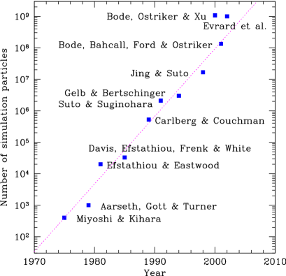
Figure 1.: Evolution of the number of particles in “high-resolution” cosmological N-body simulations.

2. 1970’s: simulating nonlinear gravitational evolution

It is not easy to identify who attempted seriously for the first time the numerical simulation of large-scale structure in the universe. Still I believe that a paper by Miyoshi & Kihara (1975) is truly pioneering, and let me briefly mention it here. They carried out a series of cosmological $N$-body experiments with $N=400$ galaxies (=particles) in an expanding universe. The simulation was performed in a comoving cube with a periodic boundary condition (Fig.2). As the title of the paper “Development of the correlation of galaxies in an expanding universe” clearly indicates, they were interested in understanding why the observed galaxies in the universe exhibit a characteristic correlation function of $g(r)=(r_{0}/r)^{s}$. In fact, Totsuji & Kihara (1969) had already found that $r_{0}=4.7h^{-1}$Mpc and $s=1.8$ is a reasonable fit to the clustering of galaxies in the Shane – Wirtanen catalogue. One of the main conclusions of Miyoshi & Kihara (1975) is that “The power-type correlation function $g(r)=(r_{0}/r)^{s}$ with $s\approx 2$ is stable in shape; it is generated from motionless galaxies distributed at random and also from a system with weak initial correlation ”.

Several years after Totsuji & Kihara (1969) published the paper, Peebles (1974) and Groth & Peebles (1977) reached the same conclusion independently, which has motivated several cosmological $N$-body simulations all over the world. Among others, Aarseth, Gott & Turner (1979) conducted a series of careful and systematic simulations to explore nonlinear gravitational clustering. Those simulations in 1970’s assume that galaxy distribution is well traced by simulations particles. In fact, the above papers spent many pages in an argument to justify the assumption, and then attempted to understand the nonlinear gravitational evolution and to quantitatively describe the large-scale structure in the computer on the basis of two-point correlation functions. In this sense, I would say that the simulations in late 1970’s are more physics-oriented rather than astronomy. Also it is interesting to mention that Prof. Kihara was a solid state physicist in the University of Tokyo and I speculate that this is why he was able to accomplish truly pioneering work from such an interdisciplinary point of view.

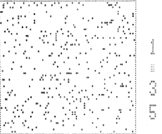
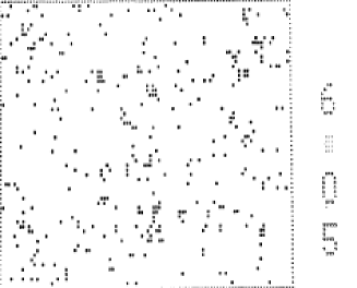
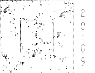
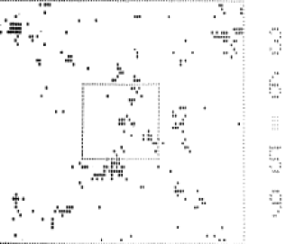
Figure 2.: Evolution of clustering from Miyoshi & Kihara (1975) at expansion factor (relative to the initial epoch of simulations) of 1.35, 6.05, 20.09 and 36.59.

3. 1980’s: introducing galaxy biasing

The primary goal of simulations of large-scale structure in 1980’s was to predict observable galaxy distribution from dark matter clustering. Necessarily one had to start distinguishing galaxies and simulation particles (designed to represent dark matter in the universe), i.e., to introduce the notion of galaxy biasing according to the current terminology. Furthermore a variety of astronomical and/or observational effects (selection function, redshift-space distortion, etc.) had to be incorporated towards more realistic comparison with galaxy redshift survey data which became available those days. Davis, Efstathiou, Frenk and White (1985) is the most influential and seminal paper in cosmological $N$-body simulations in my view. While their work is quite pioneering in many aspects, the most important message that they were able to show in a quite convincing fashion is that simulations of large-scale structure can provide numerous realistic and testable predictions of dark matter scenarios against the observational data from luminous galaxy samples. Considering the fact that they used only $N=32^{3}$ particles and thus had to identify the present epoch as when they advance the simulation merely by a factor of 1.4 relative to the initial epoch, this presents a convincing case that the most important is not the quality of simulations but those who interpret the result.

4. 1990’s: more accurate and realistic modeling of galaxy clustering

I started to work on cosmological N-body simulations around 1987, and it has been my major research topic for the next several years. At that time I often asked myself if purely N-body simulations would continue to advance our understanding of galaxy clustering significantly. My personal answer was “No. Without proper inclusion of hydrodynamics, radiative processes, star formation and feedback, it is unlikely to proceed further”, so I moved to more analytical and/or observational researches. Although I still do not think that my thought was terribly wrong, I have to admit that my decision was premature; purely N-body simulations in 1990’s turned out to be so successful and they achieved quite important contributions in (at least) three basic aspects; (i) accurate modeling of nonlinear two-point correlation functions, (ii) abundance and biasing of dark matter halos, and (iii) density profiles of dark halos, which are separately described below. Thus I returned to simulation work again in late 1990’s.

4.1. Nonlinear two-point correlation function of dark matter

The first breakthrough came from the discovery of the amazing scaling property in the two-point correlation functions (Hamilton et al. 1991). They found that the two-point correlation functions in N-body simulations can be well approximated by a universal fitting formula which empirically interpolates the linear regime and the nonlinear stable solution. Their remarkable insight was then elaborated and improved later (e.g., Peacock & Dodds 1996; Smith et al. 2003), and the resulting accurate fitting formulae have been applied in a variety of cosmological analyses.

Figure 3 plots two-point correlations of dark matter from N-body simulations (Hamana, Colombi & Suto 2001a). The symbols indicate the averages over the five realizations from simulations in real space (open circles) and in redshift space (solid triangles), and the quoted error-bars represent the standard deviation among them. The results for all particles (left panels) agree very well with the theoretical predictions (solid lines) which combine the Peacock-Dodds formula and the light-cone effect (e.g., Yamamoto & Suto 1999; Suto et al. 1999). The scales where the simulation data in real space become smaller than the corresponding theoretical predictions simply reflect the force resolution of the simulations. The result is fairly robust against the selection effect; Figure 4 indicates that the simulation results and the predictions are still in good agreement even after incorporating the realistic selection functions.

One of the main purposes of N-body simulations in 1970’s and 1980’s was to compute the nonlinear two-point correlation functions which were unlikely to predict analytically with a reasonable accuracy. In the light of this, it is interesting to note that as long as two-point correlation functions of dark matter are concerned, one does not have to run N-body simulations owing to the significant progress in semi-analytical modeling achieved on the basis of previous N-body simulations.

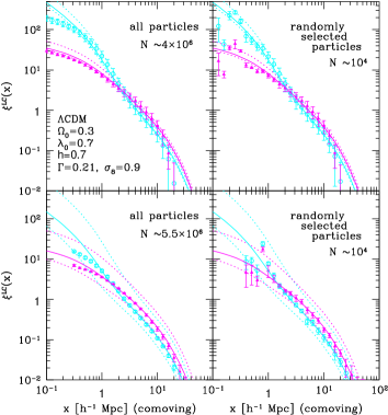
Figure 3.: Two-point correlation functions of dark matter on the light cone neglecting selection functions in $\Lambda$CDM model. Upper: $z<0.4$, Lower: $0<z<2.0$. Left: all particles, Right: randomly selected particles from the left results (Hamana, Colombi & Suto 2001a).

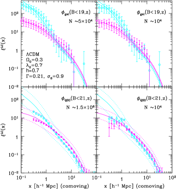
Figure 4.: Same as Figure 3 but taking account of redshift-dependent selection functions. The B-band magnitude limits of 19 (upper panels) and 21 (lower panels) are adopted so as to mimic the galaxy and QSO selection functions (Hamana, Colombi & Suto 2001a).

4.2. Biasing of dark matter halos

The second remarkable progress where N-body simulations have played a major role in 1990’s is related to the statistics of dark halos, in particular their mass function and spatial biasing. The standard picture of structure formation predicts that the luminous objects form in a gravitational potential of dark matter halos. Therefore, a detailed understanding of halo clustering is the natural next step beyond the description of clustering of dark matter particles. Both the extended Press-Schechter theory and high-resolution N-body simulations have made significant contributions in constructing a semi-analytical framework for halo clustering.

For a specific example, let me show our recent mass-, scale-, and time-dependent halo bias model (Hamana et al. 2001b):

$$b_{\rm halo}(M,R,z) = b_{\scriptscriptstyle\rm ST}(M,z)\left[1.0+b_{\scriptscriptstyle\rm ST}(M,z)\sigma_{M}(R,z)\right]^{0.15},$$ (3)

$$b_{\scriptscriptstyle\rm ST}(M,z) = 1+\frac{\nu-1}{\delta_{c}(z)}+\frac{0.6}{\delta_{c}(z)(1+0.9\nu^{0.3})},$$ (4)

which generalizes the previous work including Mo & White (1996), Jing (1998), Sheth & Tormen (1999) and Taruya & Suto (2000). The above biasing parameter is adopted for $R>2R_{\rm vir}(M,z)$, where $R_{\rm vir}(M,z)$ is the virial radius of the halo of mass $M$ at $z$, while we set $b_{\rm halo}(M,R,z)=0$ for $R<2R_{\rm vir}(M,z)$ in order to incorporate the halo exclusion effect approximately. In the above expressions, $\sigma_{M}(R,z)$ is the mass variance smoothed over the top-hat radius $R\equiv(3M/4\pi\rho_{0})^{1/3}$, $\rho_{0}$ is the mean density, $\delta_{c}(z)=3(12\pi)^{2/3}/20D(z)$, $D(z)$ is the linear growth rate of mass fluctuations, and $\nu=[\delta_{c}(z)/\sigma_{M}(R,z=0)]^{2}$.

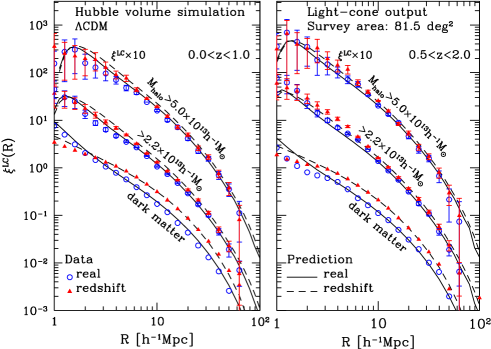
Figure 5.: Two-point correlation functions of halos on the light-cone; simulation results (symbols; open circles and filled triangles for real and redshift spaces, respectively) and our predictions (solid and dotted lines for real and redshift spaces, respectively). The error bars denote the standard deviation computed from 200 random re-samplings of the bootstrap method. The amplitudes of $\xi^{LC}$ for $M_{\rm halo}\geq 5.0\times 10^{13}h^{-1}M_{\odot}$ are increased by an order of magnitude for clarity (Hamana et al. 2001b).

Figure 5 shows the comparison of the two-point correlation functions of dark matter halos between the above semi-analytical predictions and the simulation data (Hamana et al. 2001b). For this purpose, we analyze “light-cone output” of the Hubble Volume $\Lambda$CDM simulation (Evrard et al. 2002). The two-point correlation functions on the light-cone plotted in Figure 5 correspond to halos with $M>5.0\times 10^{13}h^{-1}M_{\odot}$, $M>2.2\times 10^{13}h^{-1}M_{\odot}$ and dark matter from top to bottom. The range of redshift is $0<z<1$ (Left panel) and $0.5<z<2$ (Right panel). Predictions in redshift and real spaces are plotted in dashed and solid lines, while simulation data in redshift and real spaces are shown in filled triangles and open circles, respectively.

Our model and simulation data show quite good agreement for dark halos at scales larger than $5h^{-1}$Mpc. Below that scale, they start to deviate slightly in a complicated fashion depending on the mass of halo and the redshift range. Nevertheless the clustering of clusters on scales below $5h^{-1}$Mpc is difficult to determine observationally anyway, and our model predictions differ from the simulation data only by $\sim 20$ percent at most. This illustrates the fact that the clustering not only of dark matter but also of dark halos, at least as far as their two-point statistics is concerned, can be described well semi-analytically without running expensive N-body simulations at all.

4.3. Density profiles of dark halos

The third, and perhaps the most useful in cosmological applications, result out of N-body simulations in 1990’s is the discovery of the universal density profile of dark halos.

The study of the density profiles of cosmological self-gravitating systems or dark halos has a long history. Navarro, Frenk & White (1995, 1996, 1997) found that all simulated density profiles can be well fitted to the following simple model (now generally referred to as the NFW profile):

$$\rho(r)\propto{1\over(r/r_{\rm s})(1+r/r_{\rm s})^{2}}$$ (5)

by an appropriate choice of the scaling radius $r_{\rm s}=r_{\rm s}(M)$ as a function of the halo mass $M$. Subsequent higher-resolution simulations (Fukushige & Makino 1997, 2001; Moore et al. 1998; Jing & Suto 2000) have indicated that the inner slope of density halos is steeper than the NFW value, and the current consensus among most N-body simulators is given by

$$\rho(r)\propto{1\over(r/r_{\rm s})^{\alpha}(1+r/r_{\rm s})^{3-\alpha}}$$ (6)

with $\alpha\approx 1.5$ rather than the NFW value, $\alpha=1$ for $r>0.01r_{\rm vir}$.

Actually it is rather surprising that the fairly accurate scaling relation applies after the spherical average despite the fact that the departure from the spherical symmetry is quite visible in almost all simulated halos. A more realistic modeling of dark matter halos beyond the spherical approximation is important in understanding various observed properties of galaxy clusters and non-linear clustering of dark matter. In particular, the non-sphericity of dark halos is supposed to play a central role in the X-ray morphologies of clusters, in the cosmological parameter determination via the Sunyaev-Zel’dovich effect and in the prediction of the cluster weak lensing and the gravitational arc statistics (Bartelmann et al. 1998; Meneghetti et al. 2000, 2001).

Recently Jing & Suto (2002) presented a detailed non-spherical modeling of dark matter halos on the basis of a combined analysis of the high-resolution halo simulations (12 halos with $N\sim 10^{6}$ particles within their virial radius) and the large cosmological simulations (5 realizations with $N=512^{3}$ particles in a $100h^{-1}$Mpc boxsize). The density profiles of those simulated halos are well approximated by a sequence of the concentric triaxial distribution with their axis directions being fairly aligned:

$$R^{2}(\rho_{\rm s})=\frac{X^{2}}{a^{2}(\rho_{\rm s})}+\frac{Y^{2}}{b^{2}(\rho_{\rm s})}+\frac{Z^{2}}{c^{2}(\rho_{\rm s})}.$$ (7)

The origin of the coordinates is set at the center of mass of each surface, and the principal vectors ${\bf a}$, ${\bf b}$ and ${\bf c}$ ($a\leq b\leq c$) are computed by diagonalizing the inertial tensor of particles in the isodensity surface $\rho=\rho_{\rm s}$. Figure 6 plots the density profiles measured in this way for individual halos as a function of $R$, which indicates that equation (6) is still a good approximation if the spherical radius $r$ is replaced by equation (7). The application of the above triaxial modeling for the X-ray, Sunyaev-Zel’dovich, and lensing data is in progress (Lee & Suto 2003, 2004; Oguri, Lee & Suto 2003).

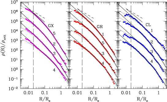
Figure 6.: Radial density profiles in our triaxial model of the simulated halos of galaxy (left), group (middle), and cluster (right) masses. The solid and dotted curves represent fits to equation (6) with $\alpha=1.5$ and 1.0, respectively. For reference, we also show $\rho(R)\propto R^{-1}$ and $R^{-1.5}$ in dashed and solid lines. The vertical dashed lines indicate the force softening length which corresponds to our resolution limit. For the illustrative purpose, the values of the halo densities are multiplied by 1, $10^{-1}$, $10^{-2}$, $10^{-3}$ from top to bottom in each panel (Jing & Suto 2002).

5. 2000’s: galaxies in cosmological hydrodynamic simulations

Although serious attempts to create galaxies phenomenologically but directly from cosmological hydrodynamic simulations have been initiated in early 1990’s (e.g., Cen & Ostriker 1992; Katz, Hernquist & Weinberg 1992), those resulting simulated galaxies are far from realistic and there are still plenty of room for improvement. Thus this is one of the most important, and yet quite realistic, goals for the simulations in the new millennium, or hopefully in this decade.

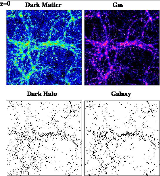
Figure 7.: Distribution of gas particles, dark matter particles, galaxies and dark halos in the volume of $75h^{-1}\times 75h^{-1}\times 30h^{-1}$Mpc³ model at $z=0$. Upper-right: gas particles; Upper-left: dark matter particles; Lower-right: galaxies; Lower-left: dark halos (Yoshikawa et al. 2001)

Let me show the result of Yoshikawa et al. (2001) for an example of such approaches. They apply cosmological smoothed particle hydrodynamic simulations in a spatially-flat $\Lambda$-dominated CDM model with particular attention to the comparison of the biasing of dark halos and simulated galaxies. Figure 7 illustrates the distribution of dark matter particles, gas particles, dark halos and galaxies at $z=0$. Clearly galaxies are more strongly clustered than dark halos. In order to quantify the effect, we define the following biasing parameter:

$$b_{\xi,i}(r)\equiv\sqrt{\frac{\xi_{ii}(r)}{\xi_{\rm mm}(r)}},$$ (8)

where $\xi_{ii}(r)$ and $\xi_{\rm mm}(r)$ are two-point correlation functions of objects $i$ and of dark matter, respectively. Furthermore for each galaxy identified at $z=0$, we define its formation redshift $z_{\rm f}$ by the epoch when half of its cooled gas particles satisfy our criteria of galaxy formation. Roughly speaking, $z_{\rm f}$ corresponds to the median formation redshift of stars in the present-day galaxies. We divide all simulated galaxies at $z=0$ into two populations (the young population with $z_{\rm f}<1.7$ and the old population with $z_{\rm f}>1.7$) so as to approximate the observed number ratio of $3/1$ for late-type and early-type galaxies.

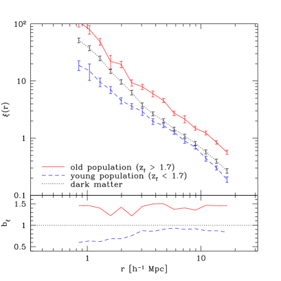
Figure 8.: Two-point correlation functions for the old and young populations of galaxies at $z=0$ as well as that of dark matter distribution. The profiles of bias parameters $b_{\xi}(r)$ for both of the two populations are also shown in the lower panel (Yoshikawa et al. 2001).

The difference of the clustering amplitude can be also quantified by their two-point correlation functions at $z=0$ as plotted in Figure 8. The old population indeed clusters more strongly than the mass, while the young population is anti-biased. The relative bias between the two populations $b^{\rm rel}_{\xi,{\rm g}}\equiv\sqrt{\xi_{\rm old}/\xi_{\rm young}}$ ranges $1.5$ and 2 for $1h^{-1}\mbox{Mpc}<r<20h^{-1}\mbox{Mpc}$, where $\xi_{\rm young}$ and $\xi_{\rm old}$ are the two-point correlation functions of the young and old populations. It is interesting to note that even this crude approach is able to explain the morphological-dependence of bias, although still in a rather quantitative manner, derived later by Kayo et al. (2004) for SDSS galaxies. With the still on-going rapid progress of observational exploration (e.g., Lahav & Suto 2003 for a recent review on galaxy redshift survey), understanding galaxy biasing as a function of galaxy properties is definitely one of the unsolved important questions in observational cosmology, and the present result indicates that the formation epoch of galaxies plays a crucial role in the morphological segregation.

6. Distribution of dark baryons

Finally let me briefly mention yet another possibility of tracing the large-scale structure of the universe using the oxygen emission lines. It is widely accepted that our universe is dominated by dark components; 23 percent of dark matter, and 73 percent of dark energy (e.g., Spergel et al. 2003). Furthermore, as Fukugita, Hogan & Peebles (1998) pointed out earlier, even most of the remaining 4 percent of the cosmic baryons has evaded the direct detection so far, i.e., most of the baryons is indeed dark. Subsequent numerical simulations (e.g., Cen & Ostriker 1999a, 1999b; Davé et al. 2001) indeed suggest that approximately 30 to 50 percent of total baryons at $z=0$ take the form of the warm-hot intergalactic medium (WHIM) with $10^{5}{\rm K}<T<10^{7}{\rm K}$ which does not exhibit strong observational signature.

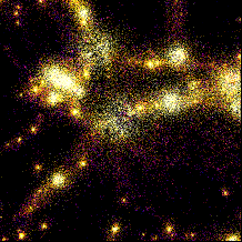
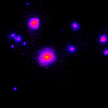
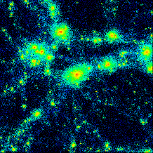
Figure 9.: Distribution of WHIM (left) compared with those of hot intracluster gas (center) and dark matter (right). The plotted box corresponds to $30h^{-1}$Mpc $\times 30h^{-1}$Mpc $\times 10h^{-1}$Mpc.

Figure 9 compares the distribution of WHIM ($10^{5}{\rm K}<T<10^{7}{\rm K}$), hot intracluster gas ($T>10^{7}{\rm K}$), and dark matter particles from cosmological smoothed-particle hydrodynamic simulations (Yoshikawa et al. 2001). Clearly WHIM traces the large-scale filamentary structure of mass distribution more faithfully than the hot gas which preferentially resides in clusters that form around the knot-like intersections of those filamentary regions. In order to carry out a direct and homogeneous survey of elusive dark baryons, we propose a dedicated soft-X-ray mission, DIOS (Diffuse Intergalactic Oxygen Surveyor; see Fig. 10). The detectability of WHIM through Oviii and Ovii emission lines via DIOS was examined in detail by Yoshikawa et al. (2003) assuming a detector which has a large throughput $S_{\rm eff}\Omega=10^{2}$ cm² deg² and a high energy resolution $\Delta E=2$ eV. Their results are summarized in Figure 11; they first create a light-cone output from the hydrodynamic simulation up to $z=0.3$, compute the bolometric X-ray surface intensity map, select several target fields and finally compute the corresponding spectra relevant for the DIOS survey. The high-spectral resolution of DIOS enables to identify the redshifts of several WHIMs at different emission energies, i.e., Oxygen emission line tomography of the WHIMs at different locations.

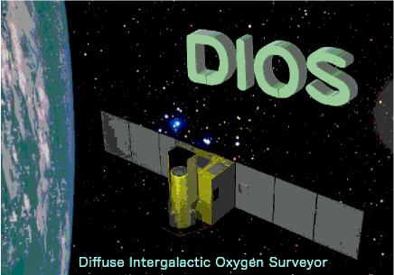
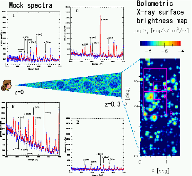
Figure 10.: A dedicated soft X-ray mission to search for dark baryons via oxygen emission lines, DIOS (Diffuse Intergalactic Oxygen Surveyor).

Figure 11.: Mock spectra of WHIMs expected for DIOS.

They concluded that within the exposure time of $T_{\rm exp}=10^{5-6}$ sec DIOS will be able to reliably identify Oviii emission lines (653eV) of WHIM with $T=10^{6-7}$ K and the overdensity of $\delta=10^{0.5-2}$, and Ovii emission lines (561, 568, 574, 665eV) of WHIM with $T=10^{6.5-7}$ K and $\delta=10^{1-2}$. The WHIM in these temperature and density ranges cannot be detected with the current X-ray observations except for the oxygen absorption features toward bright QSOs. DIOS is especially sensitive to the WHIM with gas temperature $T=10^{6-7}$K and overdensity $\delta=10-100$ up to a redshift of $0.3$ without being significantly contaminated by the cosmic X-ray background and the Galactic emissions. Fang et al. (2003) also conducted a similar study and reached quite consistent conclusions. Thus such a mission, hopefully launched in several years, promises to provide a unique and important tool to trace the large-scale structure of the universe via dark baryons.

7. Conclusions

It turned out that I was able to review the cosmological simulations only for a time-scale of decades. Still the material may be heavily biased, which I have to apologize for the organizers and possible readers of these proceedings. A millennium is definitely too long for any scientist to make any reliable prediction for its eventual outcome. Thus the number of simulation particles that I predicted in Introduction might sound ridiculous, but in reality the progress in the new millennium may be even more drastic that whatever one can imagine. For instance, it is unlikely that one still continues to use currently popular particle- or mesh-based simulation techniques over next hundreds of years. In that case, the number of particles may turn out to be a totally useless measure of the progress or reliability of simulations. Nevertheless I believe that a historical lesson that I learned in preparing this talk will be still true even at the end of this millennium; good science favors the prepared mind, not the largest simulation at the time.

Acknowledgments.

I thank Stephan Colombi, Gus Evrard, Takashi Hamana, Y.P.Jing, Atsushi Taruya, Naoki Yoshida, and Kohji Yoshikawa for enjoyable collaborations. Naoki Yoshida also encouraged me to plot Figure 1 in order to illustrate the progress of cosmological N-body simulations. I am also grateful to Ed Turner for providing me a digitized version of the first movie of his cosmological N-body simulations that I was able to present in the talk. My presentation file for the symposium may be found in the PDF format at http://www-utap.phys.s.u-tokyo.ac.jp/~ suto/mypresentation_2003e. This research was supported in part by the Grant-in-Aid for Scientific Research of JSPS. Numerical computations presented in this paper were carried out mainly at ADAC (the Astronomical Data Analysis Center) of the National Astronomical Observatory, Japan (project ID: yys08a, mky05a). DIOS (Diffuse Intergalactic Oxygen Surveyor) is a proposal by a group of scientists at Tokyo Metropolitan University, Institute of Astronautical Sciences, the University of Tokyo, and Nagoya University (P.I., Takaya Ohashi).

References

Aarseth, S.J., Gott, J.R. & Turner, E.L. 1979, ApJ, 228, 664.

Bartelmann, M., Huss, A., Colberg, J. M., Jenkins, A., & Pearce, F. R. 1998, A&A, 330, 1.

Bode, P., Bahcall, N. A., Ford, E. B., Ostriker, J.P. 2001, ApJ, 551, 15

Bode, P., Ostriker, J. P., & Xu, G. 2000, ApJS, 128, 561.

Cen, R., & Ostriker, J.P. 1992, ApJ, 399, L113.

Cen, R., & Ostriker, J. 1999a, ApJ, 514, 1.

Cen, R., & Ostriker, J. 1999b, ApJ, 519, L109.

Davé, R., et al. 2001, ApJ, 552, 473.

Davis, M., Efstathiou, G., Frenk, C.S., & White, S.D.M. 1985, ApJ, 292, 371.

Efstathiou, G., & Eastwood, J.W. 1981, MNRAS, 194, 503.

Evrard, A.E., et al. 2002, ApJ, 573, 7.

Fang, T. et al. 2003, ApJ, submitted (astro-ph/0311141).

Fukugita, M., Hogan, C.J., & Peebles, P.J.E., 1998, ApJ, 503, 518.

Fukushige, T., & Makino, J. 1997, ApJ, 477, L9.

Fukushige, T., & Makino, J. 2001, ApJ, 557, 533.

Gelb, J. M., & Bertschinger, E. 1994, ApJ, 436, 467.

Groth,E.J., & Peebles, P.J.E. 1977, ApJ, 217, 385.

Hamana, T., Colombi, S., & Suto, Y. 2001a, A& A, 367, 18.

Hamana, T., Yoshida, N., Suto, Y., & Evrard, A.E. 2001b, ApJ, 561, L143.

Hamilton, A.J.S., Matthews, A., Kumar, P., & Lu, E. 1991, ApJL, 374, L1.

Jing, Y.P. 1998, ApJ, 503, L9.

Jing, Y.P., & Suto, Y. 1998, ApJL, 494, L5.

Jing, Y. P., & Suto, Y. 2000, ApJ, 529, L69.

Jing, Y. P., & Suto, Y. 2002, ApJ, 574, 538.

Kayo, I. et al. 2004, in preparation.

Lahav, O., & Suto, Y. 2003, Living Reviews in Relativity, in press (astro-ph/0310642).

Lee, J., & Suto, Y. 2003, ApJ, 585, 151.

Lee, J., & Suto, Y. 2004, ApJ, 601, February 1 issue, in press (astro-ph/0306217).

Katz, N., Hernquist, L., Weinberg, D. H. 1992, ApJ, 399, L109.

Meneghetti, M., Bolzonella, M., Bartelmann, M., Moscardini, L., & Tormen, G. 2000, MNRAS, 314, 338.

Meneghetti, M., Yoshida, N., Bartelmann, M., Moscardini, L., Springel, V., Tormen, G., & White S. D. M. 2001, MNRAS, 325, 435.

Miyoshi, K. & Kihara, T. 1975, Publ.Astron.Soc.Japan., 27, 333.

Mo, H.J., & White, S.D.M 1996,MNRAS, 282, 347.

Moore, B., Governato, F., Quinn, T., Stadel, J., & Lake, G. 1998, ApJ, 499, L5.

Navarro, J.F., Frenk, C.S., & White, S.D.M. 1995, MNRAS 275, 720.

Navarro, J.F., Frenk, C.S., & White, S.D.M. 1996, ApJ, 462, 563.

Navarro, J.F., Frenk, C.S., & White, S.D.M. 1997, ApJ, 490, 493.

Oguri, M., Lee, J., & Suto, Y. 2003, ApJ, in press (astro-ph/0306102) .

Peacock, J.A., & Dodds, S.J. 1996, MNRAS, 280, L19.

Peebles,P.J.E. 1974, ApJ, 189, L51.

Sheth, R.K., & Tormen, G. 1999, MNRAS, 308, 119.

Smith, R. E. et al. 2003, MNRAS, 341, 1311.

Spergel, D.N. et al. 2003, ApJS, 148, 175.

Suto, Y., Magira, H., Jing, Y. P., Matsubara, T., & Yamamoto, K. 1999, Prog.Theor.Phys.Suppl., 133, 183.

Taruya, A. & Suto,Y. 2000, ApJ, 542, 559.

Totsuji, H. & Kihara, T. 1969, Publ.Astron.Soc.Japan., 21, 221.

Yamamoto, K., & Suto, Y. 1999, ApJ, 517, 1.

Yoshikawa, K., Taruya, A., Jing, Y.P., & Suto, Y. ApJ, 2001, 558, 520.

Yoshikawa, K., Yamasaki, N.Y., Suto, Y., Ohashi, T., Mitsuda, K., Tawara, Y. & Furuzawa, A. 2003, PASJ, 55, 879.