The GraF instrument for imaging spectroscopy with the adaptive optics

Abstract

The GraF instrument using a Fabry-Perot interferometer cross-dispersed with a grating was one of the first integral-field and long-slit spectrographs built for and used with an adaptive optics system. We describe its concept, design, optimal observational procedures and the measured performances. The instrument was used in 1997-2001 at the ESO 3.6 m telescope equipped with ADONIS adaptive optics and SHARPII+ camera. The operating spectral range was 1.2 - 2.5 $\mu m$. We used the spectral resolution from 500 to 10 000 combined with the angular resolution of 0.1^′′ - 0.2^′′. The quality of GraF data is illustrated by the integral field spectroscopy of the complex $0.9{\hbox{${}^{\prime\prime}$}}\times 0.9{\hbox{${}^{\prime\prime}$}}$ central region of $\eta$ Car in the 1.7 $\mu m$ spectral range at the limit of spectral and angular resolutions.

Appl. Opt. e-mail: Almas.Chalabaev@obs.ujf-grenoble.fr

1 Introduction

High angular resolution observations at the diffraction limit of the ground based large telescopes were pioneered using the speckle analysis of images [Labeyrie (1970)], however their sensitivity was severely limited by the necessity to keep exposures short in order to “freeze” the turbulence induced patterns. The adaptive optics overcame this obstacle allowing long exposures (COME-ON and ADONIS at the ESO 3.6 m telescope, adonis97, PUEO at the CFHT, pueo98, NAOS at the ESO VLT, lagrange03, and others). The limiting magnitude on the telescopes equipped with the adaptive optics (hereafter AO) is now defined by the detector and optics efficiency as for any observations, while the angular resolution is close, at least in the IR, to the telescope diffraction limit, about 0.1^′′ for a 4 m aperture at $\lambda=2$ $\mu m$.

The achievements of the AO were firstly exploited for imaging (see reviews by close00, lai00, menard00). The next step was to use the adaptive optics for spectroscopy. Indeed, the combination of high angular and high spectral resolutions is a key issue for a number of observational programmes such as physics and evolution of multiple stellar systems, morphology and dynamics of circumstellar gas and jets in young and evolved stars, etc.

Driven by this ideas, the GraF project was started in 1995 with the aim to build an imaging spectrograph optimized for the use with the ADONIS at the ESO 3.6 m telescope. The instrument is based on the integral field spectroscopic properties of the Fabry-Perot interferometer (hereafter FPI) used in cross-dispersion with a grating (le Coarer et al., 1992, 1993). It was tested at the telescope in 1997 and successfully used for a number of astronomical programmes in 1998-2001 (for preliminary results see Chalabaev et al., 1999a, 1999b, 1999c, trouboul99).

In the present article we describe in details the optical concept and the instrument built to fit the constraints imposed by ADONIS Beuzit et al. (1997) and the SHARPII+ camera Hofmann et al. (1995). We give the account of the observational procedures emerged from our experience as optimal, present the measured performances, and illustrate them by a sample of reduced data obtained at the limit of the instrument possibilities in terms of the angular and spectral resolutions.

The discussion will be restricted to the applications of a high spectral resolution ($R\simeq 5000$ - $10000$) in a moderate passband ($\Delta\lambda\leq 50$) combined with a high angular resolution ($\simeq$ 0.1^′′ - 0.2^′′) in a small field of view ($FOV\leq 15{\hbox{${}^{\prime\prime}$}}$). The operating spectral range of the instrument was $1.2\,-\,2.5$ $\mu m$.

We hope that this one of the first experiences of the imaging spectroscopy with the adaptive optics (see also tiger95, lavalley97) will be useful for designers and users of future spectro-imaging instruments combining the high angular and high spectral resolutions.

2 Image restoration aspects

Let us in what follows to make the emphasis of the discussion on the scarcely resolved objects, i.e. having the spatial spectrum in the Fourier domain comparable in the extent to that of the AO corrected telescope modulation transfer function (MTF).

There are two reasons for such a choice. Firstly, as witnessed by the reviewers (cf. close00, lai00, menard00), the AO provides a considerable scientific contribution mainly in the case where the object under study, having remained point-like at lesser angular resolutions, becomes scarcely resolved, revealing new spatial features.

The second reason is dictated simply by the fact that the scarcely resolved objects are the most difficult to measure, so that the overall performance of a new instrument at the limit of resolution is best evaluated on such objects.

We can already note that the importance of the scarcely resolved objects shapes the specifications on the AO assisted spectrograph. Indeed, to recover the information up to the highest possible spatial frequency implies the image restoration, and this aspect has necessarily to be taken into account in the design of the spectrograph.

2.1 General

We shall consider the flux density distribution $S(x,y,\lambda)$ which is non-zero at least at 2 points of the two-dimensional (2D) sky field {$x,y$}. Here, $x$ and $y$ are the spatial coordinates, and $\lambda$ is the wavelength. As it was already said in Sect. 1, the discussion will be restricted to small fields, $\leq 15{\hbox{${}^{\prime\prime}$}}$.

The image restoration problem of imaging spectroscopy in the general case consists in finding the best estimate ${\hat{S}}(x,y,\lambda)$ of the object flux distribution density $S(x,y,\lambda)$, satisfying the tri-dimensional integral equation of convolution:

$$F(x,y,\lambda)=\int{}\int{}\int{}d\xi d\zeta dw\cdot S(\xi,\zeta,w)\cdot{\cal{G}}(\xi-x,\zeta-y,w-\lambda)$$ (1)

where $F$ is the measured flux density distribution and $\cal{G}$ is the instrumental impulse response.

The solution of the integral equation of convolution is known to be unstable (turchin71; see also lucy94review). The calibration errors of $\cal{G}$ are strongly amplified in the final result of image restoration, in particular at high frequencies, so that the solution $\hat{S}$ has to be regularized, i.e. searched in a space of appropriate smooth functions (see for details tikhonov77, titterington85, lucy94strategy).

The image restoration can be carried out using either one of the many proposed deconvolution algorithms (e.g. cornwell92, magain98, lucy03, and references therein), or by modeling $\hat{S}$ from a priori defined physical considerations and then searching for the best fit of the convolution product $\hat{S}\otimes{\cal{G}}$ to $F$ within the physical model.

It is clear that whatever the method adopted for the image restoration, the accurate calibration of $\cal{G}$ is of high importance. Let us analyze the sources of the calibrations errors in the case of imaging spectroscopy in order to get guidelines of the instrumental concept.

2.2 Calibration errors

Firstly, we can simplify the Eq.(1) by noting that for the considered here angular fields, spectral passbands and resolutions (see Sect. 1) the 3D impulse response $\cal{G}$ can be written as the product of the spatial point-spread function (psf) ${\cal{P}}(x,y|\xi,\zeta;\lambda)$ and the instrumental spectral profile ${\cal{L}}(x,y;\lambda|w)$ (see e.g. perina, goodman68, mariotti). Then we get:

$$F(x,y,\lambda)=\int{}dw\cdot{\cal{L}}(x,y,\lambda-w)\int{}\int{}d\xi d\zeta\cdot S(\xi,\zeta,w)\cdot{\cal{P}}(\xi-x,\zeta-y,\lambda)$$ (2)

We will further assume that the relevant scientific information can be extracted without deconvolution on $\lambda$. In other words, we will limit the discussion to the frequently encountered case where the instrumental spectral profile ${\cal{L}}$ is much narrower than the studied spectral lines.

We can then write:

$${\cal{L}}(x,y,\lambda-w)\simeq L(x,y,\lambda)\cdot\delta(\lambda-w)$$ (3)

where $L(x,y,\lambda)$ is the spectral transmission, a simple multiplicative factor, and $\delta(\lambda-w)$ is the Dirac impulse function.

The convolution concerns now only the spatial dimensions, so that the Eq.(2) is further simplified as follows:

$$F(x,y,\lambda)=L(x,y,\lambda)\int{}\int{}d\xi d\zeta\cdot S(\xi,\zeta,\lambda)\cdot{\cal{P}}(\xi-x,\zeta-y,\lambda)$$ (4)

The important consequence is that in the absence of the deconvolution on $\lambda$ the contribution of the calibration errors on ${\cal{L}}$ to the uncertainty of the final estimate $\hat{S}$ is considerably reduced.

Furthermore, we note that usually the variations of $\cal{L}$ during observations are due to mechanical flexure at the telescope. They are slow, with the time scale of tens of minutes, and can be monitored with a good accuracy. Similarly, the dependence of $\cal{L}$ on $x$ and $y$ is stable and can be calibrated accurately.

In contrast to the relative stability of ${\cal{L}}$, the psf ${\cal{P}}$ undergoes significant temporal variations on the time scale of minutes or even shorter due to atmospheric turbulence. Although the AO improves dramatically the situation, the residual wavefront variations can still be significant. Their amplitude depends on the operating wavelength, the amplitude and the time scale of the atmospheric turbulence, the performances of the AO system and the telescope aperture size. With the ESO 3.6 m telescope and the ADONIS, the variations of ${\cal{P}}$ expressed in terms of the Strehl ratio were found to change from 10 to 35 in the K band for the seeing value of $\approx 1.5{\hbox{${}^{\prime\prime}$}}$ within the time interval of 10 $s$ (adonis_lemignant). The variability is a fortiori stronger at the shorter wavelengths of J and H bands.

As to the wavelength dependence of ${\cal{P}}$, it is negligible within the considered here spectral range of a single instrument setting, $\Delta\lambda/\lambda\leq 50$.

We can conclude that the main source of errors in the final result of image restoration, the flux distribution estimate $\hat{S}$, comes from the calibration of the spatial psf ${\cal{P}}$ due to its rapid variability. The way it is calibrated needs thus special attention. For instance, the calibration errors can be substantially reduced if ${\cal{P}}$ is measured simultaneously with the measurement of $F$, e.g. on a suitable source in the same field. If ${\cal{P}}$ can be measured only on a source off the field, it must be done as close in time as possible. The instrumental concept has to take into account these observational aspects.

It also appears important that the two-dimensional $\{x,y\}$-structure of the field and of the psf $\cal{P}$ is recorded with no scanning on $\{x,y\}$, in order to keep the error on $\cal{P}$ homogeneous over $x$ and $y$, thus avoiding a random scrambling of spatial features, which can be unrecoverable.

As to the spectral response $\cal{L}$, the contribution of its calibration errors in the final uncertainty on $\hat{S}$ is considerably lesser than that of $\cal{P}$. Indeed, the instrumental spectral profile $\cal{L}$ is relatively stable and can be calibrated much more accurately than ${\cal{P}}$. Furthermore, if no deconvolution is justified on $\lambda$, i.e. if the spectral resolutions high enough, then the error on $\cal{L}$ propagates into the error on $\hat{S}$ without amplification.

2.3 Implications for the AO assisted spectroscopy

The above given analysis provides the guidelines of the instrumental concept for the AO assisted imaging spectroscopy which can be briefly summarized as follows: (i) the calibration of the psf $\cal{P}$ has to be simultaneous, or as close in time as possible, to the measurement of the flux distribution $F$; (ii) the scanning over the spatial $x$- and $y$-axes must be avoided; (iii) if scanning is unavoidable due to the volume of data to be recorded, the instrument concept allowing $\lambda$-scanning is preferable.

Obviously, the ideal spectro-imaging instrument would record the entire cube of data $F(x,y,\lambda)$ in one single exposure with no scanning, satisfying the criteria of both the accurate image restoration and the saving the telescope time.

The work is in progress on the “3D detectors” able to record both the position ${x,y}$ and the energy $\lambda$ of the photons, cf. the superconducting tunnel junctions (stj94, stj00) or the dye-doped polymers (shbd95). However, their sensitivity is still less convincing than that of the modern 2D-detectors.

The best available today solutions are offered by the optical set-ups known as the integral field spectrographs (IFS, courtes82, tiger95, mpi3d94, vimos98, spiffi00). They use the 2D detectors to record $F(x,y,\lambda)$ with no scanning, provided the detector size is large enough to record the 3D data cube at once.

3 Particular case of a “linear image”

Let us also consider the simplest case of the imaging spectroscopy when the object flux density $S(x,y,\lambda)$ is non-zero along a straight line, so that $S$ is a function of only two variables, $S(x,\lambda)$.

In this “linear” case, frequently encountered in the astrophysical practice (e.g. binary stellar systems), the common grating spectrographs recording $F(x,\lambda)$ at a single setting offer a suitable solution, insuring the calibration of psf ${\cal{P}}$ homogeneous over the studied field {$x$}. Furthermore, in the case of a circumstellar nebular object, when the extended feature is a gas emitting only in spectral lines, the emission in the continuum corresponds to the point-like star and provides the calibration of ${\cal{P}}(x)$ simultaneous to the measurement of $F$.

4 The minimum 3D data cube volume

At high angular and high spectral resolutions, the volume of data to be recorded in one observation of imaging spectroscopy can be large. Let us to estimate what is its minimum under typical astrophysical specifications.

Empirically, the angular field of $\simeq 3{\hbox{${}^{\prime\prime}$}}\times 3{\hbox{${}^{\prime\prime}$}}$ would be adequate to study most types of objects of interest of the stellar physics. The pixel size of 0.05^′′ is fixed by the angular resolution, which is $\approx 0.1{\hbox{${}^{\prime\prime}$}}$ at a 4 m telescope at $\lambda=2\,\mu$m. Thus, the record of the spatial flux distribution at a given wavelength $F_{\lambda}(x,y)$ consists of $60\times 60=3600$ data values. Along the $\lambda$-axis, the minimum of about 100 points is suitable in order to record the profile of a spectral line and the adjacent continuum. Thus, the entire cube data volume is at least $60\times 60\times 100\simeq 600^{2}$ values.

This largely exceeds the $256^{2}$ size of the detector available with ADONIS/SHARPII+. In our case the IFS approach is clearly unaffordable, the scanning is imposed. Then, in agreement with the conclusions of error analysis in imaging spectroscopy given in Sect. 2.3, we adopted the concept of the $\lambda$-scanning imaging spectrograph described below.

5 The GraF concept

5.1 Optical scheme. Data cube structure

The concept uses a Fabry-Perot interferometer in cross-dispersion with a grating (hence the acronym we gave for this concept, GraF = Gra(ting) and F(abry-Perot). The set-up (see Fig. 1) was first described by fabry, and used for spectroscopy by chabal and kulagin80. The IFS property of the set-up was noticed by elc-phd and demonstrated by le Coarer et al. (1992, 1993). baldry went further, describing a tunable echelle imager, where a FPI is cross-dispersed with a grism and with an echelle grating.

In a single frame, GraF records the quasi-monochromatic images of the field $F_{\lambda}(x,y)$ corresponding to several values of $\lambda$, which is the distinctive property of an IFS instrument. The spectrum is sampled by a comb of the FPI transmission peaks (interference orders) separated by the interorder wavelength spacing $\Delta\lambda_{f}$ (Sect. 6). The whole set of $\lambda$ values is recovered by scanning.

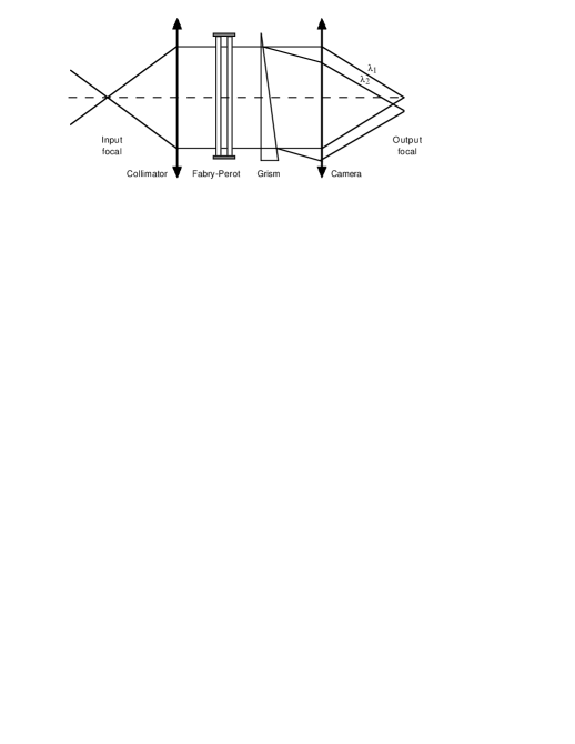
Figure 1: The optical concept of the the imaging spectrograph using a Fabry-Perot interferometer in cross-dispersion with a grating, replaced here by a grism for the convenience of the drawing.

The structure of the spectro-imaging data cube is illustrated in Fig. 2. The FPI acts as a “multi-passband” filter. The light of different FPI orders is sorted by the grating according their wavelength. The resulting series of quasi-monochromatic images of the sky field is formed in the output focal plane. Note that the width of the entrance field must be limited by a focal aperture to avoid superposition of order images.

Anticipating a detailed discussion (Sect. 6), let us give the figures of a typical cube volume recorded with the actually built instrument. At each step of scanning, the detector frame of $256^{2}$ pixels records 8 narrow-band images corresponding to the dispersed sequence of the FPI orders as selected by the grating angle value. Each FPI “order image” covers the same 1.5^′′$\times$12.4^′′ region of the entrance sky field sampled with the pixels of 0.05^′′, which makes $\simeq 30\times 250=7440$ spatial pixels.

This is close to the estimated minimum required by the stellar observations, although, the width of the FOV $\simeq$ 1.5^′′ is a factor of 2 less than the desirable $\simeq 3{\hbox{${}^{\prime\prime}$}}$ value. For the observations of the elongated objects, this shortage is partially compensated by the considerable height of the FOV of $\simeq 12{\hbox{${}^{\prime\prime}$}}$, which can be suitably aligned.

The spectral band covered by the detector is about 40 nm at $\lambda=2.2$ $\mu m$, corresponding to 8 FPI orders. It is scanned in 48 FPI channel frames, although in special cases one can limit the scan to a narrower range of interest. The number of spectral samples in a full FPI scan is $48\times 8=384$. The spectral passband of an image is $\delta\lambda\simeq 0.3$ nm at $\lambda$=2 $\mu m$, so that the corresponding spectral resolving power is $R=\lambda/\delta\lambda\simeq 7000$. The total volume of the cube is $48\times 256^{2}=3.15\cdot 10^{6}$ pixels, or $\simeq 1770^{2}$ pixels.

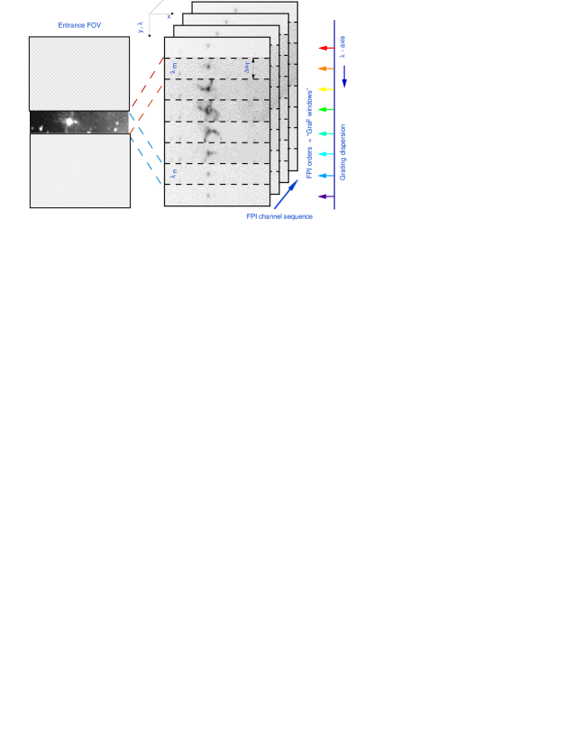
Figure 2: The structure of the GraF IFS cube. Left: The “Southern Crab” planetary nebula as it appears in the white light (simulated). The field of view is limited by a rectangular entrance aperture. Right: The images of the nebula in the light of a atomic spectral line (simulated image) as they appear in the focal plane of the GraF instrument. Each frame consists of several monochromatic “windows” corresponding to the FPI orders. Due to the differential motion of the nebulae, the aspect of the nebula is changing from one “window” to another.

5.2 Advantages and limitations of the concept

The GraF $\lambda$-scanning IFS appears as a suitable solution when scanning is imposed by the modest detector size. It allows a simultaneous record of several monochromatic images of a reasonably large field thus keeping possible an accurate image restoration.

Scanning is done by the comb of spaced FPI transmission peaks rather than by a contiguous set of the wavelength values like in a grating based instrument. The peaks spacing makes more certain to have in each frame at least one “order” image placed at the wavelengths of the continuum emission, thus providing a reference signal for photometric monitoring and, in the nebular cases, the calibration of the ${\cal{P}}$ simultaneous to the measurement of $F$.

Another convenient point of the concept is the simplicity of transforming a grating spectrograph into a GraF instrument by adding solely a FPI and an adjustable slit (see also comments by baldry). Vice versa, the instrument is easily switched to a grating spectrograph for observations of “linear” objects.

However, the GraF concept is intrinsically scanning, so that if scanning is unnecessary, the GraF is slower than other mentioned above IFS concepts.

Further, the width of the FOV has an upper limit. Expressed in the elements of the angular resolution $\delta\phi$, the FOV width cannot exceed the FPI finesse value $\cal F$ (see Sect.  6.2). For the maximum $\cal F$ of $\simeq 40$ still suitable for the high-throughput imaging (bland95), the maximum FOV width of a GraF is $\simeq 4{\hbox{${}^{\prime\prime}$}}$ for $\delta\phi\simeq 0.1{\hbox{${}^{\prime\prime}$}}$.

6 Formulae for GraF optical parameters

6.1 FPI formulae

Let us remind the basic terms describing the FPI properties. The FPI spectral transmission is a comb of peaks, called “orders”, occurring at $\lambda_{m}$ defined by the condition of the interference:

$$m\lambda_{m}=2ne\cos i$$ (5)

where the integer $m$ is the order of the interference, $n$ the refractive index, $e$ the gap between the FPI plates, and $i$ the angle of incidence.

The value of $\lambda_{m}$ varies over the FOV according to the value of $i$. However, as it can be estimated from Eq. 5, this variation is negligible: ${\delta\lambda}/{\lambda}\simeq 5\cdot 10^{-9}$ for the considered fields of view $\leq$ 15^′′. In what follows, it will be assumed that $i=90$^∘, so that the gap $e$ defines completely the set of $\lambda_{m}$.

The distance between two neighbor orders is called the interorder spectral spacing. Expressed in the wavelength units, $\Delta\lambda_{f}$, it can be written from Eq. 5 as follows:

$$\Delta\lambda_{f}=\frac{\lambda_{m}\lambda_{m+1}}{2ne}\simeq\frac{\lambda^{2}}{2ne}$$ (6)

It is often more convenient to use the interorder spacing expressed in the wavenumber units $\Delta\sigma_{f}$, which has no spectral dependence:

$$\Delta\sigma_{f}=\frac{1}{2ne}$$ (7)

The element of spectral resolution $\delta\lambda$ will be defined as the $FWHM$ of the instrumental profile $\cal{L}$. It has the advantage to be immediately measurable (see however jones_bland95 for different criteria of resolution).

The effective finesse $\cal{F}$ is defined as the ratio of the interorder spectral spacing to the element of spectral resolution:

$${\cal F}=\frac{\Delta\lambda_{f}}{\delta\lambda}$$ (8)

The instrumental profile $\cal{L}$ is the Airy function:

$${\cal{L}}=\frac{1}{1+{\cal{F}}sin^{2}(\pi\sigma/\Delta\sigma_{f}}$$ (9)

For high values of $\cal{F}$, it can be approximated by the Lorentzian:

$${\cal{L}}=\frac{1}{1+(2\sigma/\delta\sigma)^{2}}$$ (10)

Using Eqs.(6) and (8), the spectral resolving power $R=\lambda/\delta\lambda$ can be formally written as follows:

$$R=\frac{2ne\cal F}{\lambda}$$ (11)

Given that the finesse $\cal F$ approximately corresponds to the number of the effective reflections on the FPI plates, the maximum optical path difference between the interfering wavefronts $OPD_{max}$ can be written as follows:

$$OPD_{max}\approx 2ne{\cal{F}}$$ (12)

The sampling step we used for the FPI scanning is $h=\delta\lambda/2.7$. This appears as “oversampling” as compared to the “canonic” value of $h_{s}\simeq 2$.

There are two ways to justify the used value of $h$. The first one is to argue that the Airy profile of $\cal{L}$ has a considerably sharper core than the more familiar Gaussian or $sinc^{2}$ profiles of grating spectrographs, so that the rate based on the convention $\delta\lambda=FWHM$ would certainly undersample the core profile.

More strictly speaking, let us recall that the step $h$ allowing to fully interpolate the function with a finite Fourier spectrum must be $h\leq h_{s}=1/(2\cdot f_{cut})$ (Shannon theorem), where $f_{cut}$ is the cut-off frequency of the Fourier spectrum. It happens that for a Gaussian profile, $\delta\lambda=FWHM\simeq 1/f_{cut}$, which conveniently translates into “the rule” $h_{s}=\frac{1}{2}\delta\lambda$. The trouble with FPI is that the Fourier transform of $\cal{L}$ is never zero and has no $f_{cut}$. Thus, formally FPI escapes the Shannon theorem.

In practice, the effective number of reflexions on the FPI plates, hence the effective finesse $\cal{F}$ and the effective $OPD_{max}$, is limited by the noise, so that $f_{cut}$ can be defined on this basis. For the same instrument, it will vary depending on the S/N ratio. The uncertainty on $f_{cut}$, and hence on $h_{s}$, explains the choice of a conservatively small value of $h=\delta\lambda/2.7$.

6.2 GraF formulae. The limits and optimum for the FOV width

In the absence of the grating, the output image would be a superposition of all images transmitted in the passbands of the FPI orders. The grating deviates each order light into a specific angle according to its wavelength $\lambda_{m}$, and thus spatially sorts the order images (see Fig. 2).

In the output focal plane, the shift between the order images $\Delta w_{f}$ is equal to the interorder spectral spacing $\Delta\lambda_{f}$ scaled by the reciprocal dispersion $rdisp$ (expressed in $nm/pix$) as follows:

$$\Delta w_{f}~{}~{}\textstyle{[pix]}=\frac{\Delta\lambda_{f}}{rdisp}$$ (13)

Since the axis of $\lambda$ in the output focal plane is collinear with the spatial $y$-axis, the value of $\Delta w_{f}$ can be also expressed in $arcsec$ through the platescale $H$:

$$\Delta w_{f}~{}~{}\textstyle{[arcsec]}=P\cdot\frac{\Delta\lambda_{f}}{rdisp}$$ (14)

Albeit shifted according their wavelength, the order images superimpose. The confusion is finally avoided by limiting the width of the entrance FOV to the value $\Delta w_{f}$. The latter, expressed in $arcsec$, is the confusion free width of the FOV, or simply the free width (see Fig. 2).

The Eq.(13) seems to indicate that the free width $\Delta w_{f}$ can be increased arbitrarily by increasing the grating spectral dispersion. However, the extension of the output psf along the $\lambda$-axis, measured as the FWHM $\delta\phi_{graf,disp}$, also increases with the dispersion due to collinearity of $\lambda$- and $y$ axes.

We can write:

$${\cal{P}}_{graf,disp}=\int{}dw\cdot(M_{FP}(w)\cdot{\cal{P}}_{ao}(w)){\cal{L}}_{gr}(w-\lambda)$$ (15)

where ${\cal{P}}_{graf,disp}$ is the psf profile along the $\lambda$-axis at the GraF output, ${\cal{P}}_{ao}(\lambda)$ is profile of the monochromatic psf at the output of the adaptive optics, $M_{FPI}$ is the spectral transmission of the FPI, and ${\cal{L}}_{gr}(w-\lambda)$ is the instrumental spectral profile of the grating.

For the corresponding FWHM’s, we get :

$$\delta\phi_{graf,disp}~{}~{}\textstyle{[pix]}\simeq\sqrt{\delta\phi_{ao}^{2}+\left(\frac{\delta\lambda}{rdisp}\right)^{2}}$$ (16)

which gives the explicit relation of $\delta\phi_{graf,disp}$ and $rdisp$.

To get the insight into the tradeoff guiding the choice of the spectral dispersion value $rdisp$, let us introduce the dimensionless free width of FOV, $\Delta w_{el}$, expressed in the number of the spatial elements of resolution $\delta\phi_{graf,disp}$ as follows:

$$\Delta w_{el}=\frac{\Delta w_{f}}{\delta\phi_{graf,disp}}\simeq\frac{\frac{\Delta\lambda_{f}}{rdisp}}{\sqrt{\delta\phi_{ao}^{2}+\left({\frac{\delta\lambda}{rdisp}}\right)^{2}}}$$ (17)

From the last equation and Eq.(8), it follows that when the spectral dispersion increases, i.e. $rdisp\rightarrow 0$, then:

$$\Delta w_{el}\rightarrow\Delta w_{el,max}=\frac{\Delta\lambda_{f}}{\delta\lambda}={\cal F}$$ (18)

The finesse ${\cal F}$ sets the asymptotic upper limit to the number of spatial elements that one can get along the width of the GraF FOV. This is illustrated in Fig. 3, which displays the ratio of $\Delta w_{el}$ to the possible maximum $\Delta w_{el,max}$ in function of the spectral sampling ratio along the grating dispersion $\rho_{\lambda}$. The latter is defined as the number of pixels for one element of resolution, $\rho_{\lambda}=\delta\lambda/rdsip$. The curves are computed for several values of the spatial sampling ratio, $\rho_{s}=\delta\phi_{ao}/H$.

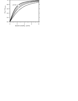
Figure 3: The ratio of the free width expressed in number of resolution elements $\Delta w_{el}$ to its asymptotic maximum $\Delta w_{el,max}={\cal F}$ in function of the spectral (along the grating dispersion) and spatial sampling ratios.

One can see that $\Delta w_{el}/\Delta w_{el,max}$ increases rapidly up to $\rho_{\lambda}\simeq 2.5$ and saturates afterwards. The range of $rdisp$ and $\Delta w_{f}$ corresponding to $\rho_{\lambda}\simeq 2.5$ can be considered as optimum. Higher dispersions will give only a slight increase of $\Delta w_{el}/\Delta w_{el,max}$, while the number of order windows covered by the detector, $M_{wind}$, will decrease linearly.

The numerical values of the free width $\Delta w_{f}$ chosen for the instrument are close to the optimum. They and are given in Tab. 3 in $arcsec$ and $pixels$. The corresponding value of $\Delta w_{el}$, for instance at $\lambda=2.2~{}\mu$m, is $\Delta w_{el}\approx 7$. The other parameters are the platescale $H=50$ $mas/pix$ (hereafter $mas$ states for $milli-arcseconds$), $rdisp$ of the 300 mm^-1 grating, the free width $\Delta w_{f}$ = 1.55^′′ and the measured psf extension $\delta\phi_{graf,disp}=0.22{\hbox{${}^{\prime\prime}$}}$ (see Sect. 10.1).

The maximum possible width at this wavelength is $\Delta w_{el,max}={\cal F}\approx 16.8$, as calculated from $\Delta\lambda_{f}=4.75$ nm and the measured spectral resolution $\delta\lambda=0.3$ nm of the FPI. The measured ratio $\Delta w_{el}/\Delta w_{el,max}\approx 0.45$ is close to the theoretical value of 0.55 derived from Fig. 3 for the used spatial and spectral samplings ratios respectively $\rho_{s}=2.6$ and $\rho_{\lambda}=1.9$.

7 Implementation at the telescope

7.1 Hardware

The implemented spectrograph has been designed to meet the ADONIS imposed mechanical constraints, dictating a compact (1.5 m $\times$ 0.5 m) and light (30 kg) instrument (see Fig. 4). The operating wavelength range from 1.2 $\mu m$ to 2.5 $\mu m$ corresponds to that of the SHARPII+ camera.

The spectrograph was installed at the ADONIS visitor equipment bench (adonis97), located between the adaptive optics output and the SHARPII+ camera. The flat mirror M_in intercepts the ADONIS f/45 output beam and sends it into the spectrograph. The beam passes firstly through a field rotator made of a prism and a flat mirror. The field rotator of GraF allows to vary the slit orientation on the sky, which otherwise would have been remained fixed due to ADONIS constraints.

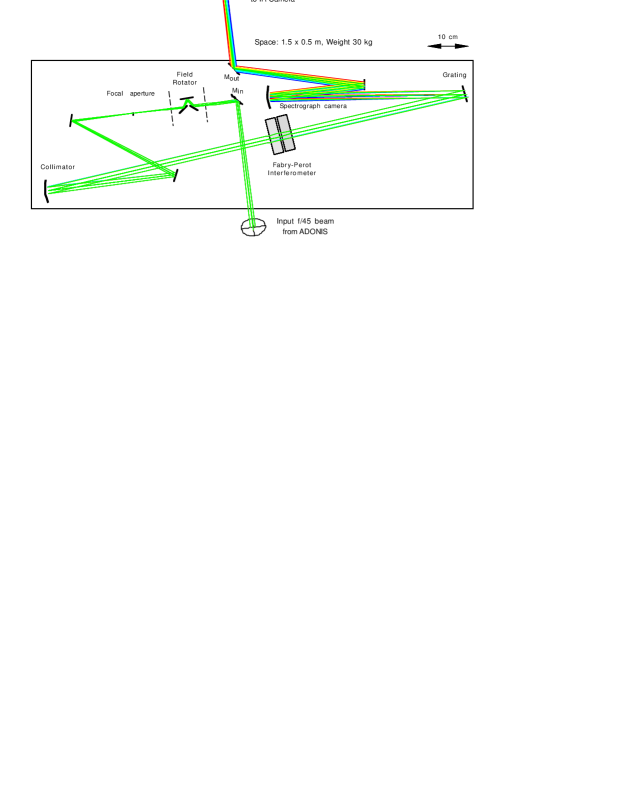
Figure 4: The GraF optical design.

The FOV is selected by the rectangular aperture located in the ADONIS focal plane. Its width, can be adjusted continuously and with a good precision from 0.1^′′ to 15^′′, and its height is fixed to about 30^′′. After the aperture, the beam is collimated, passes through the Fabry-Perot interferometer, is dispersed by the grating, reconfigured by the spectrograph camera back to the f/45 beam and sent to the SHARPII+ camera.

The instrument can also be used in a direct imaging mode, either by setting the grating at the zero order position, or replacing it by a flat mirror mounted at the back of the grating (not shown in Fig. 4). In this configuration the FPI is used in the classical scanning mode.

The two flat mirrors M_in and M_out, located on the axis of the ADONIS-SHARPII+ camera, are mounted on a dedicated common support, so that they can be removed and installed within minutes, allowing a quick change from the GraF IFS mode to the regular ADONIS imaging observations.

The motors controlling the focal aperture, the field rotator, the grating position, the FPI in- and out- of the beam movements, are operated through the GraF dedicated version of the ADOCAM real-time operations software written by F. Lacombe. The GraF operation at the telescope thus inherited conveniently from the user-friendly interface of the wide-band imaging ADONIS observations, and in particular the possibility to launch the command sequences in the batch mode.

7.2 Optical quality

The necessity to fit the instrument into a reduced room implied adding 5 more flat mirrors in the optical design, further, the necessity of the field rotator implied adding 3 mirrors more. In total, it makes 11 reflecting surfaces. The loss in transmission is limited by the high efficiency golden coatings. However, this extra number of optical surfaces certainly decreased the spectrograph image quality. Estimating that a mirror is manufactured with $\lambda/10$ precision, and $\lambda=0.6$ $\mu m$, the accumulated $rms$ wavefront error should be about 200 $nm$, or $\lambda/5$ at the shortest operating wavelength of $1.2$ $\mu m$, which can be considered as still acceptable.

More importantly, these static aberrations, at least at low and moderate spatial frequencies, are corrected by the fine tuning of the AO, so that the degradation of the final image quality is negligible as witnessed by the stellar images given in Fig. 7. The AO tuning is done at the beginning of each night.

7.3 Observing modes

The Table 1 summarize the observing modes of the GraF instrument. It shows an apparently complex instrument, while in practice the change from one mode to another is done in a few dozen of seconds or in a few minutes at longest, and can be programmed beforehand using the ADONIS/ADOCAM control software scripts. The availability of the modes of direct imaging and of grating spectroscopy (hereafter GS) was very valuable during the tests, providing independent and complementary measurements for the IFS mode. Furthermore, the GS mode was extensively used for observations of “linear” objects like binary stars.

The grating is mounted on a high quality turning support, so that the grating angle settings are of a high precision insuring an accurate and stable wavelength setting. This was of special importance for the IFS mode. Indeed, during the FPI scanning the image on the detector undergoes slight shifts along the $\lambda$-axis. We used an automatic procedure compensating these shifts by changing the grating angle at each change of channel in order to keep the image as precise as possible at the same detector pixels and thus to decrease the uncertainties of the flux estimate.

7.4 Optical parameters

The spectral resolutions are listed in Tab.  2.

Mode	Focal aperture	FPI	Grating position
Direct Imaging	Open	Out	Zero order, or
	J & H: 9′′ $\times$ 9′′		Flat mirror
	K: 12.8′′ $\times$ 12.8′′
Grating spectros.	Open, or narrow slit	Out	chosen $\lambda$
	J & H: $\simeq$0.2′′ $\times$ 9′′
	K: $\simeq$0.2′′ $\times$ 12.8′′
Scanning IFS	Rectangular	In	chosen $\lambda$, compensation
	J & H: $\simeq$0.8′′ $\times$ 9′′		of the $\lambda$-shift induced
	K: $\simeq$1.5′′ $\times$ 12.8′′		by the FPI scan
Scanning FPI	Open	In	Flat mirror
imaging spectroscopy	J & H: 9′′ $\times$ 9′′
	K: 12.8′′ $\times$ 12.8′′

Table 1: The summary of the available observing modes.

$\lambda(\mu$m)	IFS and FPI modes	Grating Spectroscopy
		35 mm-1	300 $mm^{-1}$	600 $mm^{-1}$
1.25	16000	200	1200	2500
1.65	10000	300	1600	3500
2.2	7000	600	4000	10000

Table 2: Spectral resolving power. For the grating spectroscopic mode, it corresponds to the slit width of 0.2^′′.

The Table  3 gives the main parameters of the GraF IFS mode: the reciprocal dispersion $rdisp$, the free FOV width $\Delta w_{pix}$ and $\Delta w_{arc}$, and the number of order windows covered by the detector, $M_{ord}$. The parameters are listed for the 2 gratings available in the IFS mode and for the mostly used platescale $H=50$ mas/pix. The parameters for two other available platescales, 35 mas/pix and 100 mas/pix, can be obtained by applying the scaling factor, except $\Delta w_{arc}$ which does not depend on $H$.

The FPI, fabricated by Queensgate Inc. according to our specifications, has the following parameters: the interorder spectral spacing 10.1096$\pm$0.0005 $cm^{-1}$, the finesse ${\cal F}$ about 20 depending on the wavelength, the optical transmission in peaks about 85%. The FPI has two operating spectral ranges, $\lambda\lambda$ $1.2\,-\,2.5$ $\mu m$ and $\lambda\lambda$ $3.8\,-\,4.5$ $\mu m$, due to the plates coating proposed by E. le Coarer. Only the first range was used with the GraF/ADONIS instrument.

7.5 Thermal background

The thermal background of a non-cooled spectrograph is significant at $\lambda>2$ $\mu m$. It was the subject of a special analysis during the design phase. Let us remind that the main source of the thermal emission is the warm environment of the grating. Indeed, contrary to a mirror with the bi-univocal correspondence between the incoming and reflected beams, a grating has more than one order of interference and consequently more than one input lobes corresponding to the output beam. It is a well known problem in the visible spectroscopy solved by limiting the detector passband by an order blocking filter. To reduce the thermal background, we adopted a similar solution, so that as a rule the spectroscopy at $\lambda\lambda$ $2-2.5$ $\mu m$ was done using the cooled circular variable filter (CVF) (see sharp95). Its passband $\lambda/\Delta\lambda\simeq 50$ fitted nicely the spectral range covered by the NICMOS detector with the 300 $mm^{-1}$ grating the most frequently used in the IFS mode.

$\lambda$	Grating 300 $mm^{-1}$				Grating 600 $mm^{-1}$
	Disp.	Free FOV width		$M_{ord}$	Disp.	Free FOV width		$M_{ord}$
$\mu m$	nm/pix	arcsec	pix		nm/pix	arcsec	pix
1.2	0.1655	0.43	8.70	29	0.0767	0.94	18.8	13
1.6	0.1621	0.79	15.8	16	0.0707	1.81	36.2	7
2.2	0.1558	1.55	31.1	8	0.0581	4.17	83.3	3
2.5	0.1520	2.06	41.1	6	0.0494	6.32	126.5	2

Table 3: Parameters of the IFS order window for the platescale 50 mas/pix. The FPI interorder spectral spacing $\Delta\sigma_{f}=10.1096$ $cm^{-1}$.

7.6 Measured sensitivity

The measured limiting magnitudes $m_{lim}$ in the two main spectroscopic modes are listed in Table 4. In the J and H bands, $m_{lim}$ is very close to the values derived from the limiting magnitudes of the broad-band imaging Le Mignant et al. (1999) and the theoretical GraF throughput of 0.64 for the GS mode and of 0.54 for the IFS mode. The throughput was calculated taking the reflexion coefficient of 7 mirrors equal to 0.98 each, the transmission of the FPI of 0.85, the efficiency of the grating of 0.80, and the transmission of the field rotator of 0.94. In the K band, for the exposures shorter than 1 min in the GS mode and 5 min in the IFS mode, the noise is dominated by the detector read-out noise ($\simeq 35$ electrons); above this time, the noise is dominated by that of the thermal background.

Mode	Exp. time (min.)	J	H	K
IFS	1	8.5	9.4	9.3
	5	10.4	11.1	10.0
Grating	5	10.6	11.4	10.6
Spec.	30	12.1	12.9	11.5

Table 4: The measured limiting magnitudes for S/N=5 with the grating 300 $mm^{-1}$. The integration time for the IFS mode is given per frame. For the grating spectroscopy, the values are given for the slit width of 0.2^′′. The spectral resolutions are those of Table 2.

8 Observing procedures and calibrations

We will limit the discussion of the observing procedures to the IFS mode and to particularities of the GS mode, other modes being classical.

8.1 Grating long slit and slitless spectroscopy

The sharpness of the AO psf ${\cal{P}}$ with $\delta\phi\simeq 0.1{\hbox{${}^{\prime\prime}$}}~{}-~{}0.2{\hbox{${}^{\prime\prime}$}}$, much steeper than that of seeing limited observations (e.g. racine_psf), is a new element to take into account for the GS observations. Setting the slit width close to the extension of ${\cal{P}}$ as it is usually done for seeing limited observations, can give rise instrumental effects which could be neglected so far, like e.g. diffraction at the slit border. With the rapidly variable psf $\cal{P}$, these effects are difficult to calibrate. Also, the acquisition of the star on the center of the slit of only $\approx$ 0.1^′′ - 0.2^′′ wide can take considerable telescope time.

To avoid these losses, we let whenever possible the entrance aperture wide open (several arcsec), the sharpness of ${\cal{P}}$ already insuring a well defined spectrum. The important caution in this slitless mode of observations was to take a direct image of the field to record the accurate positions of the star(s) producing the spectrum (see Fig. 5). The difference of the stellar $y$-positions relative to the middle of the slit provides then the value of the translation to be applied to the wavelength calibration obtained as usually on a calibration spectral lamp with a narrow slit.

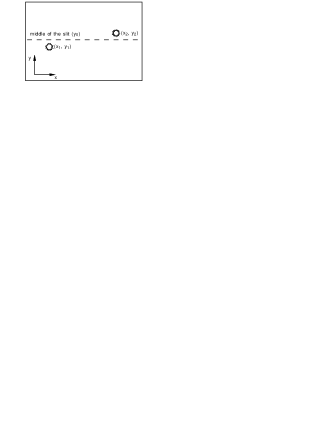
Figure 5: The entrance field of view in the slitless GS-spectroscopic mode operation. A direct imaging exposure giving the $y$-positions of the stars relative to the middle of the slit allows to adjust the zero’s of the wavelength scales of the stellar spectra.

8.2 Calibrations

The main instrumental effects implying the calibration exposures were the usual detector pixel-to-pixel response and bias values, and the spectral setting parameters. The complete set of GS data of an object is as follows (with the typical global telescope time given in parenthesis):

• Scientific long slit or slitless GS frame (10-30 min);

• Image frame of the spectroscopic field of view; Particularly important for slitless GS to define the translation of the wavelength calibration (1 min);

• Long slit spectrum of the “flat-field” produced by a tungsten lamp illuminating the entrance ADONIS pupil; gives the calibration of the detector pixel-to-pixel variations of sensitivity; the slit width 0.2^′′ -  0.4^′′ (needs the interruption of the AO servo-loop, 5 min);

• Long slit spectrum of a spectral Ar or Ne lamp, providing the wavelength calibration; the slit width 0.2^′′ (1 min, done during the same interruption of the AO servo-loop as the “flat-field” spectrum);

While the wavelength calibration was reliable and better than 0.01% (see Sect. 10.1), the “flat-field” calibration of the pixel-to-pixel variations of sensitivity turned out to be troublesome. It turned out that the design of the SHARPII+ camera optics and that of the NICMOS detector conspired in the way to modulate the overall spectral response by the interference fringes formed by the sapphire substrate of the detector (see Fig. 6). At some wavelengths, the amplitude of the fringes was up to 20% peak-to-peak. More importantly, the fringe pattern could vary, by translation due to probably mechanical flexure, and also due to variations of the NICMOS pixels sensitivity. It was therefore mandatory to take the “flat-field” spectra very close in telescope position and time to the object spectrum. With all cares taken, the residual fringing was still about 1%, and sometimes worth.

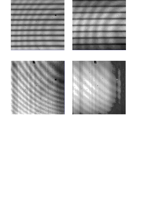
Figure 6: Flat-field frames in the 3D-mode (top) and in the long slit mode (bottom), at $\lambda=1.6$ $\mu m$ (left), and at $\lambda=2.2$ $\mu m$ (right).

A typical IFS data set is as follows:

• The IFS cube of data on the object (from 20 min for exposures of 15 s per frame up to about 1 hour for 60 s per frame);

• Direct image of the field of view (1 min);

• IFS “flat-field” cube (5 - 10 min);

• IFS spectral lamp cube, with the FPI scanning limited to about 10 steps around a prominent spectral line of Ar or Ne, providing the IFS cube wavelength calibration and the measurement of the FPI spectral response (5 min).

The parallelism of the FPI plates is checked and adjusted in the beginning of each night.

9 Data reduction

Although the deconvolution is an integral part of the spectrum extraction in the case of scarcely resolved objects (see Sect. 2), a complete discussion of the possible strategies in different types of situations is largely out of the scope of the present paper. Here, we will describe only the procedures used to extract the spectra of the complex central region of $\eta$ Car object chosen to test the instrument performances at the limit of the resolution.

9.1 Preliminary steps

They were as follows:

• The frame “cleaning” for irrelevant pixel values. It was done using a median filter with the adaptive threshold and the area size, which can run along columns, lines, or square areas according to best final result. The irrelevant pixel values were replaced by the 2-dimensional linear interpolation.

• Dark frames subtraction;

• Flat-field division.

9.2 Spectrum extraction. GS mode

Since at the beginning of every run the detector was aligned so that its lines were parallel to the the slit. The grating dispersion is then parallel to the detector columns at least in first approximation. However, the parabolic aberration usual to grating spectrographs makes a stellar spectrum to be a slightly curved line. We therefore extracted the spectra of stellar sources by fitting the psf ${\cal{P}}$ line by line, with the multiplicative factor $A$ (amplitude) and the position across the dispersion as the fit parameters. The amplitude $A$ gives the estimate $\hat{S}$ of the flux density. The psf ${\cal{P}}$ is the average of several lines selected in the continuum of an isolated star, if possible the studied object, otherwise a reference star off the field.

If the spectrum was obtained as a slitless (see Sect. 8.1), the calibration of the line number vs the wavelength $\lambda$ is done taken into account the position of the star with respect to the slit center.

The spectrum of a standard star in Fig. 9 (dotted line) gives an example of the final result.

9.3 Spectrum extraction. IFS mode

9.3.1 Isolated stars

The spectrum extraction for an isolated star is done by fitting a two-dimensional normalized psf ${\cal{P}}$ to each order image of a channel frame with the amplitude $A$ and the $\{x,y\}$ position as the fit parameters. As in the GS case, the amplitude $A$ is used as the estimate $\hat{S}$ of the flux density $F$, and after the wavelength calibration the vector $\hat{S}$ vs $\lambda$ provides then the stellar spectrum (Fig. 9, solid line).

The psf ${\cal{P}}$, constructed as the “shift-and-add” average of the images corresponding to the stellar continuum, is normalized so that the integral of the signal over the psf area is equal to one. This normalization makes the fit amplitude insensitive to the variations of the Strehl ratio from one channel frame to another.

If each channel frame contains orders corresponding to the stellar continuum, then one can monitor the channel-to-channel photometric variations. Obviously, the continuum orders must be selected as free as possible from the telluric absorptions. The channel-to-channel variations of the average flux are assumed then to be photometric and give the correction factor. The method was successfully tested on the data of HR8353 (see Sect. 10.1).

9.3.2 Complex objects with the features at the psf scale

The deconvolution becomes then unavoidable. Comparison of different strategies being out of the scope of the present article, we can give only a short description of the recipes used during the data reduction of the test case of the $\eta$ Car central region (see Sect. 10.2

Firstly, the psf ${\cal{P}}$ is constructed as described for the isolated stars cases. Then the Richardson-Lucy (RL) deconvolution algorithm was run on the cube frames. The RL algorithm provides a sharpened image clarifying the structure of the object. However, the resulting flux distribution is unreliable for the quantitative analysis (e.g. magain98), and must be found by other methods.

So that at the next step we used a simple physical modeling of the studied region best fitting the data. Thus the model for $\eta$ Car consisted of point sources at the positions found by RL algorithm.

The distance between the secondary spots in $eta$ Car, down to 0.11arcsec, being too close to the resolution limit (0.11arcsec at $\lambda$ 1.7$\mu m$), the uncertainties of the model fitting turned out to be too important to be used for the spectrum extraction.

We used then a specific to $\eta$ Car additional information provided by the photocenter spectral dependence in the way known as the differential “super-resolution” (beckers82, toko92). This allowed us to separated the spectrum of the bright star and the remaining secondary objects (see for details Sect. 10.2).

9.3.3 Software

We used the Khoros 2.1 software integration and development environment, which provides the visual programming of data flows and an extended library of routines suitable for the reduction and analysis of data up to 5 dimensions KRI (1996). When necessary, GraF specific routines were developed and added to the Khoros library .

10 Example and quality of the IFS data

We present and discuss below the instrument performances in terms of spectroscopic and imaging capabilities measured in two relevant test cases.

The first case is a single standard star. Its measurement provides a reliable estimate of the quality of the spectrum extracted from the IFS data. We show in particular that recording the stellar light simultaneously in several spectral “windows” allows to accurately monitor the channel-to-channel variations of flux count estimates.

The second case is the observation of the central 0.9^′′$\times$0.9^′′ region of $\eta$ Car, well studied by previous research groups. It provides an excellent test of spectro-imaging ability of the instrument in a complex field with the spatial structure at scales down to the limit of the angular resolution (about 0.1^′′) as well as the spectral line profile structure at scales close to the limit of the GraF spectral resolution (about 10 000 in this case).

10.1 Spectrum of a standard star

A IFS set of data on a standard star HR8353 B3III, K = 3.31 mag van der Bliek et al. (1996) was obtained in November 1997. The spectral range covering about 40 nm was centered on the hydrogen Br-$\gamma$ 2165.55 nm line. The FPI interorder spectral spacing of about 4.75 nm was covered by 48 FPI channel frames with the spectral step between the channels of 9.895$\cdot 10^{-2}$ nm as measured in the FPI order m = 457. We used the SHARPII+ platescale of 50 mas/pix and the grating of 300 $mm^{-1}$ (see Tab.  3 for other parameters). One channel frame records here 8 FPI order images, the total number of spectral points is thus 48$\times$8 = 384. The exposure time per channel was 10 s.

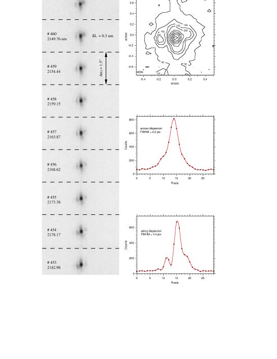
Figure 7: A channel frame of the IFS cube of the standard star HR5383.
Left panel: The central strip of the frame corrected for the detector bias and pixel-to-pixel sensitivity variations. The dashed lines indicate the spatial limits of the FPI order windows. The spectral passband of window $\delta\lambda$ = 0.3 nm, or R $\simeq$ 7000. Right panel: The point-spread function extracted from the order 459. Top: The contour map of the stellar image. The contour decrement is 100 counts above the 200 counts level. Middle and bottom: The counts distribution through the maximum respectively across and along the spectral dispersion; the FWHM $\delta\phi_{x}$ = 2.6 pix (0.13^′′), and $\delta\phi_{graf,disp}$ = 4.4 pix (0.22^′′).

A strip with the stellar images recorded in the first channel is reproduced in Fig. 7 (left). The good image quality of GraF data is witnessed by the sharpness of the flux distribution with FWHM $\simeq$ 0.13^′′ across the grating spectral dispersion, as one would expect for the diffraction limited image. Along the dispersion, FWHM $\simeq$ 0.22^′′, as one expects for the convolution product of the diffraction limited image with the spectral response of the FPI and the grating (see Sect. 6.2 and Eq.(16)).

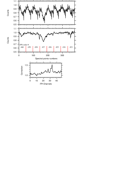
Figure 8: Correction for the “photometric” variations during the FPI scan.
Top and middle: Flux counts estimate in the channels before (top) and after (middle) the correction for counts variations. The FPI order numbers and their spectral limits are indicated in the middle plot. The scan consists of 48 channels. One channel covers 8 FPI orders, the scan results in 384 spectral points. The points are numbered in the order of the increasing wavelength. Bottom: The photometric correction vs channel.

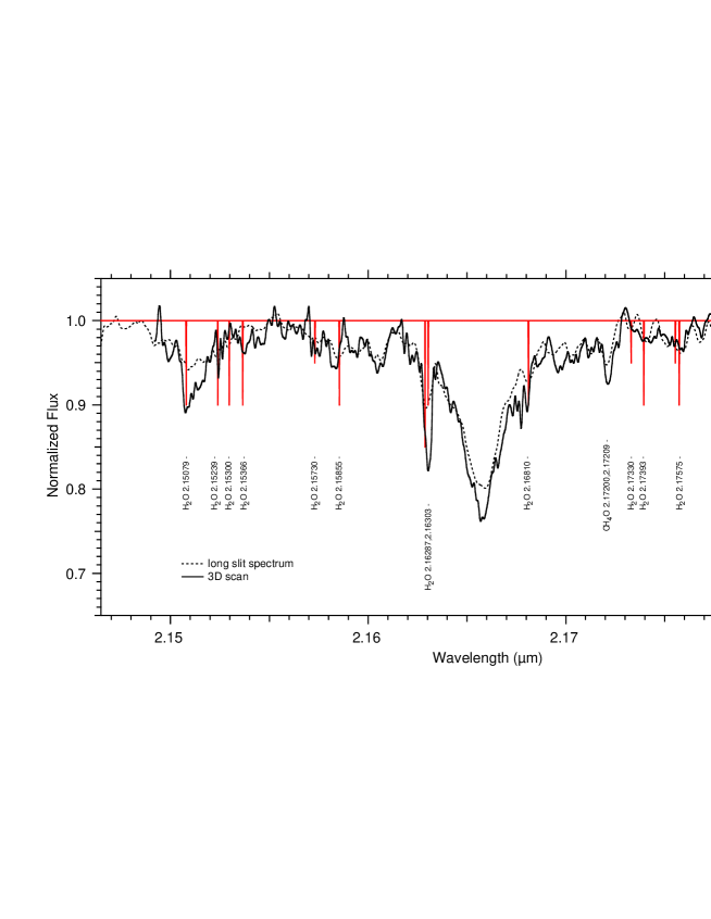
Figure 9: Spectrum of a standard star HR8353 extracted from the IFS cube, corrected for the channel-to-channel counts variations and calibrated in wavelength. The spectrum obtained in the long slit mode is also plotted as the dashed line. The identified telluric lines are indicated by vertical bars.

The data reduction steps after the usual bias subtraction and correction for the pixel-to-pixel variations were as follows. Firstly, the psf ${\cal{P}}$ was estimated separately for each channel as the “shift-and-add” average of the stellar images in the continuum. Then the flux count in each order window was estimated by fitting ${\cal{P}}$ to the stellar images, with the flux count and the image photocenter as the free parameters. The flux estimate in function of the spectral point number is plotted in Fig. 8 (top). The spectral point numbers are in the order of increasing $\lambda$. One can see strong variations of the flux estimate correlated with the channel number.

We selected the order windows free of stellar and telluric spectral lines, and imposed the condition such that the total stellar flux in those windows is the same for all channels, which is the definition of the stellar continuum. The channel-to-channel variations of the so defined total flux are then ascribed to the photometric variations, and used to calculate the correction factor plotted in Fig. 8 (bottom). Applying the correction factor to the extracted spectrum resulted in the rectified spectrum shown in Fig. 8 (middle) and Fig. 9.

In fact, the described channel-to-channel variations were mostly due to the method used for the flux estimate, the psf ${\cal{P}}$ fitting, which is sensitive to the Strehl ratio, varying with time. Using other methods, e.g. integrating on the area of the stellar image gives much better results. However, we took profit of this data reduction misadventure to demonstrate the possibility of accurate correction of photometric variations.

The wavelength calibration accuracy was estimated by measuring the agreement between the expected and the measured positions of the telluric lines. It was excellent with the relative rms error in $\lambda$ being 4$\cdot$10^-5.

The S/N ratio estimate is biased by the numerous at this sensitivity faint ($\leq$1% of the continuum) telluric absorptions due to H₂0, CH₄, etc., mostly identified in Fig. 9, using the tables by mohler55. The lower limit S/N $>$ 100 (1 standard deviation) was measured on 50 points of on the less contaminated spectral interval starting from $\lambda 21800$ nm. An additional estimate was obtained from the GS data recorded as a sequence of 10 identical exposures. The variations of the flux counts from one exposure to another gave the estimate S/N$\simeq 300$, close to the expected from the photon statistics for this bright star.

10.2 Imaging spectroscopy of multiple spots in the $\eta$ Car central region

The $\eta$ Car object is a luminous star loosing mass in giant eruptions (see review by davidson_araa97). The central region contains several point-like sources as illustrated in Fig. 10, the bright spot A of $\eta$ Car, and the B, C and D spots at the distance 0.1^′′ - 0.3^′′ to the NW from the central star (weigelt86). davidson97, using HST/GHRS, obtained the UV-spectroscopy of the B, C and D spots, showing them to be dense, compact slow-moving ejecta emitting in narrow forbidden emission lines of FeII. The stellar core emits in broad permitted emission lines formed in the dense fast stellar wind (see also hamann94 for the ground-based spectroscopy of $\eta$ Car with the angular resolution $\delta\phi\approx 5{\hbox{${}^{\prime\prime}$}}$ and the spectral resolution R $\approx$ 3000 in the near IR, and hillier01 for the HST/STIS spectrum of $\eta$ Car spot A in the the 164 - 1040 nm spectra range with $\delta\phi\approx 0.25{\hbox{${}^{\prime\prime}$}}$ and R up to 5000).

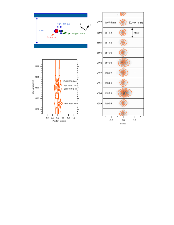
Figure 10: Imaging spectroscopy of $\eta$ Car in the 1668-1692 nm range. Left top: The FOV of the IFS cube. Left bottom: The long slit spectrum; the slit width 0.2^′′, spectral resolution $\simeq$3500. The contours are at 500, 1500, 2500, 3500 and 4500 counts. Right The channel frame 44 of the $\eta$ Car IFS cube. The FOV and the spectral settings are indicated; spectral resolution $\simeq 10000$.

10.2.1 Observations

The observations of $\eta$ Car were done on Nov. 15, 1997 at UT 9:00-9:20. We selected the spectral range 1668-1692 nm, since it fortunately includes several spectral transitions of various excitation, namely the hydrogen Br11 1680.6 nm, [FeII] 1676.9 nm, FeII 1678.7 nm, and FeII 1687.3 nm Hamann et al. (1994). The overview of the spectrum is given by the long slit spectroscopy frame (Fig. 10) taken with the slit centered on the spot A and turned to the positional angle PA=311^∘, between those of the B and C spots at PA=340^∘ and PA=296.5^∘ respectively Hofmann and Weigelt (1988). The exposure time was 15 s, and the spectral resolution $R\simeq$ 3500.

The IFS data were taken with the platescale 35 mas/pix and the grating 300 $mm^{-1}$. The FOV width was 0.86^′′, and the height 9.0^′′. The height is fixed by the detector format. The positional angle of the IFS observations was the same as for the GS data, PA=311^∘. The cube consisted of 48 channel frames of the FPI. Each channel frame records the FOV in 9 order windows with the passband $\delta\lambda=0.16$ nm each, or R = 10 000. The exposure time per channel was 5 s.

The instrumental performances in terms of the image quality and deconvolution can be illustrated and discussed on the example of one channel frame. The full set of data will be presented and discussed elsewhere together with its astrophysical implications.

10.2.2 Deconvolution

Already the visual inspection of the cube shows that at the wavelengths of [FeII] 1676.9 nm, FeII 1678.7 nm and 1687.3 nm lines the $\eta$ Car image is extended. For the following discussion we selected the channel frame 44, where the emission in these lines is at maximum (see Fig. 10, orders 593 and 590, corresponding respectively to FeII 1678.7  nm and 1687.3 nm). On the other hand, the $\eta$ Car image in the continuum emission, orders 595-597, is that of a point-like source, so that we could select one of the orders, namely 596, as the psf ${\cal{P}}$ for the deconvolution.

The frame was deconvolved using the Richardson-Lucy maximum likelihood algorithm (lucy74, hook94), stopped after 50, 200 and 1000 iterations. The results obtained with 200 iterations were selected as the best compromise between the attained resolution and the level of artifacts. They are displayed in Fig. 11.

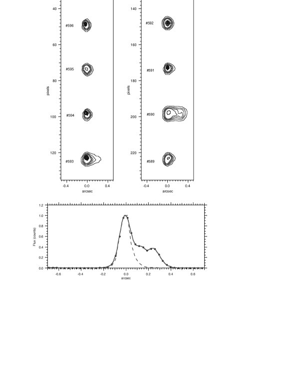
Figure 11: Top: The deconvolved $\eta$ Car image in the channel frame 44. Bottom: The flux profiles across the spectral dispersion in the orders 590 (solid line) and 589 (dashed line). The profiles are normalized to the maximum value. The secondary maxima in the order 590 are at 0.13^′′ and 0.24^′′ from the maximum flux.

The regular and sharp appearance of the stellar image in the order 591, produced by solely continuum emission and therefore corresponding to the unresolved stellar core, witnesses the good quality of the deconvolution and absence of artifacts. The FWHM of this image is 0.1^′′, very close to the diffraction limit of the telescope.

In contrast, the image in the FeII line order 590 shows a complex structure. The flux profile across the dispersion (Fig. 11, bottom) has two secondary maxima, at 0.13^′′ and 0.24^′′ from the primary. This is in a good agreement with the values of 0.114^′′ and 0.211^′′ given for B and C spots by hofmann88, indicating thus the good quality of the deconvolved GraF data. The D spot is not seen probably due to its faintness.

10.2.3 Spatially resolved spectra

To complete the task of the imaging spectroscopy as it was discussed in Sect. 2, we have to solve the image restoration problem and find the set of estimates ${\hat{S}}(x,y,\lambda)$ of the flux density distribution.

Unfortunately, the Richardson-Lucy deconvolution does not restore properly the flux distribution, enhancing artificially the sharp sources.

We therefore tried the model fit method. The flux distribution estimate $\hat{S}$ was modeled as as set of monochromatic functions ${\hat{S}}_{\lambda}(x,y)$ consisting of a primary point-like object surrounded by 1, 2 or 3 secondary point-like objects. The model function is then convolved with $\cal{P}$ and we look for $\hat{S}$ giving the best fit to the observed flux distribution $F_{\lambda}(x,y)$. However, no fit gave satisfaction, either showing too high residuals (models with 1 and 2 secondaries), or a too shallow likelihood maximum (models of 3 secondaries) implying highly uncertain fluxes and positions.

This is not very surprising given that the separation of the A, B and C spots is very close to the angular resolution limit of the telescope $\delta\phi\simeq 0.1{\hbox{${}^{\prime\prime}$}}$ at this wavelength.

The way turned to be fruitful was taking into account the additional information provided by the photocenter spectral dependence, following the ideas of the differential “super-resolution” approach (beckers82, toko92). The Fig. 12 displays the integrated spectrum of the whole 0.9^′′$\times$0.9^′′ region in the FeII 1687.3 nm line (top), and the photocenter (center of gravity) position across the dispersion vs wavelength (bottom). The photocenter remains constant all along the continuum emission and along the broad wings of the FeII line. It deviates up to 150 mas in strong correlation with the narrow spectral emission appearing at the top of the broad spectral line.

The spectra are separated if we assume a simple model where $\eta$ Car is composed of 2 objects: the unresolved bright primary (spot A) and an “ejecta cloud”, which includes both the B and C spots and, possibly, a halo. Indeed, then the photocenter drift indicates that the the broad emission comes from the spot A, while the narrow emission well correlated with the deviation of the photocenter comes from the “ejecta cloud”.

Figure 12: Top: The profile of FeII 1687.3 nm in the spectrum of $\eta$ Car. Bottom: The corresponding drift of the photocenter vs wavelength.

One can derive the parameters of the “cloud” emission as follows: FWHM $\simeq$ 80 km$\cdot$s^-1 and FWZM $\simeq$ 180 km$\cdot$s^-1. The broad emission of the primary spot A has FWZM $\simeq$ 900 km$\cdot$s^-1. The ratio of the total flux emitted in the line by the “cloud” to that of the primary is about 0.4. The “cloud” emission in the FeII 1678.6 nm line has similar properties.

The presence of emission of two kinds in the near IR lines, one with a large velocity dispersion, coming from the stellar wind, and another with a low velocity dispersion, has been already reported by hamann94, who suggested that the first one may arise in a disk surrounding the star. The GraF data obtained at a higher spectral and spatial resolutions showed for the first time the velocity resolved profile of the narrow FeII 1676.9 nm emission and clearly indicate that it arises in the ejecta composed of B and C spots to the NW from the bright primary A, in a good qualitative agreement with the work of davidson97.

Clearly, more information can be extracted from the present data, using additional spectral lines, etc. This will be presented in a forthcoming article, the discussion of this section being a mere illustration of the instrument performances.

11 Conclusions and prospects

The GraF instrument for imaging spectroscopy based on the Fabry-Perot interferometer in the cross-dispersion with a grating was successfully tested and operated at the 3.6 m telescope with the ADONIS adaptive optics, allowing to combine the spectral resolution up to 10 000 with the high angular resolution of 0.1^′′ - 0.2^′′ provided by ADONIS. The ability of simultaneous imaging in several spectral passbands proved to allow in certain cases the simultaneous calibration of the spatial point-spread function ${\cal{P}}$. The subsequent deconvolution of data in the crowded field of $\eta$ Car is shown to be of a high quality, with the final angular resolution close to 0.1^′′ at $\lambda=1.7~{}\mu$m, close to the telescope diffraction limit, in spite of the fact that at this rather short wavelength the adaptive optics correction of the atmosphere induced wavefront perturbations was only partial, and the point-spread function was highly variable in time.

The simultaneous mapping of $\eta$ Car with resolutions R up to 10 000 and $\delta\phi\approx$ 0.1^′′ achieved from the ground with ADONIS/GraF in the 1.7 $\mu m$ spectral range compares favorably with R up to 5 000 and $\delta\phi\approx$ 0.1^′′ obtained on the same object with the space-born instrument HST/STIS in the visible and far-red spectral range Hillier et al. (2001).

In its practical aspects, the optical concept of the FPI cross-dispersed with a grating proved to be compact and versatile, allowing to switch to the long-slit spectroscopy, or to direct imaging within a minute.

The potential of the GraF concept has been further proven by the construction of new instruments either adopting its principles as the GriF scanning integral-field spectrograph for the CFHT (grif00, grif02), or developing them further as the Tunable Echelle Imager (baldry).

High quality data were obtained during the period of the scientific use of the instrument at the telescope in 1998-2001 on different programmes of stellar physics. They will be a subject of forthcoming papers.