Proper motion surveys of the young open clusters Alpha Persei and the Pleiades

In this paper we present surveys of two open clusters using photometry and accurate astrometry from the SuperCOSMOS microdensitometer. These use plates taken by the Palomar Oschin Schmidt Telescope giving a wide field ($5^{\circ}$ from the cluster centre in both cases), accurate positions and a long time baseline for the proper motions. Distribution functions are fitted to proper motion vector point diagrams yeilding formal membership probabilities. Luminosity and mass functions are then produced along with a catalogue of high probability members. Background star contamination limited the depth of the study of Alpha Per to $R=18$. Due to this the mass function found for this cluster could only be fitted with a power law ($\xi(m)=m^{-\alpha}$) with $\alpha=0.86^{+0.14}_{-0.19}$. However with the better seperation of the Pleiades’ cluster proper motion from the field population results were obtained down to $R=21$. As the mass function produced for this cluster extends to lower masses it is possible to see the gradient becoming increasingly shallow. This mass function is well fitted by a log normal distribution.

1 Introduction

The young open cluster Alpha Per lies at a distance of 183 pc ($(M-m)_{o}=6.31$, van Leeuwen 1999) with an age of 90 Myr (Stauffer, Barrado & Bouvier 1999). We assume in this paper that $A_{R}=0.23$(O’Dell, Hendry & Collier Cameron 1994). It has been reasonably well studied in the past using various techniques. Prosser’s catalogue (Prosser 1993) contains a comprehensive list of candidate member stars identified by photometry, spectroscopy and radial velocity measurements. The faintest of these has $V\approx 21.8$($M_{V}\approx 15.5$). These candidate stars have been supplemented by those identified in similar studies by Zapatero Osorio et al. (1996), Stauffer et al. (1999) and Rebolo et al. (1992). In addition Prosser, Randich & Simon (1998) identified candidate stars which were optical counterparts to X-ray sources within the cluster.
An early proper motion study by Heckmann, Dieckvoss & Kox (1956) identified stars with proper motions consistent with cluster membership. However this study only went down to $V\approx 12$ and did not calculate formal membership probabilities. Prosser (1992) also used stellar proper motions as an initial selection technique. Although this study was deeper than the earlier one ($V=18.8$) it also did not calculate formal membership probabilities.
Most recently Barrado y Navascués et al (2001) produced a deep CCD survey of the cluster. This identified several candidate low mass stars and Brown Dwarfs down to $I_{c}=22$. They then used this data to produce a mass function. The mass function was fitted with a power law whose slope was found to be $\alpha=0.59$.
The Pleiades is the best studied open cluster, here we assume $(M-m)_{o}=5.4$ (van Leeuwen 1999) and $A_{R}=0.15$ (O’Dell, Hendry & Collier Cameron 1994). In recent years several deep CCD surveys of the cluster such as Dobbie et al (2002) and Moraux et al (2003) have produced candidates down to $0.03M_{\odot}$. These have been complimented by proper motion studies such as those of Hambly et al (1999) and Moraux, Bouvier and Stauffer (2002). However the only wide field, high precision proper motion survey is that of Hambly, Hawkins and Jameson (1991). Adams et al (2001) used 2MASS data along with proper motions to produce a wide field study. This contained many candidate stars outside the tidal radius of the cluster showing background star contamination is a problem for many techniques.

Figure 1: A plot showing the sky coverage of the Alpha Per study. The solid line represent the later POSSII fields while the dotted lines are the earlier POSSI fields. The dashed circles marks out a five degree radius from the cluster centre (marked by an x).

Figure 2: A plot showing the sky coverage of the Pleiades study. The solid line represent the later POSSII fields while the dotted lines are the earlier POSSI fields. The dashed circles marks out a five degree radius from the cluster centre (marked by an x).

2 Observational data and reduction

2.1 Obseravtions

The SuperCOSMOS facility at the Royal Observatory Edinburgh has (using plates from the United Kingdom Schmidt Telescope) produced complete southern sky surveys in $B_{J}$, $R$ and $I$ with an additional second epoch $R$ survey. These surveys are now publicly available (Hambly et al 2001). The scanning program has now moved on to the northern hemisphere, using film and glass copies of plates taken by the Oschin Schmidt Telescope on Mount Palomar, California. These data will soon be publicly available. The declination of Alpha Per ($\delta\approx 49^{\circ}$) and the Pleiades ($\delta\approx 24^{\circ}$) means this prerelease northern hemisphere data must be used. Details of these plates are given in Table 1 for Alpha Per and Table 2 for the Pleiades. Unfortunately due to saturation caused by the bright core stars of the cluster and a satellite track, 3.1% (2.3 sq deg) of the Pleiades survey area was unusable. The region of the CO cloud near Merope was used in the proper motion survey, it is assumed that the increased reddening in this region will not affect the results. The areas covered by both surveys are shown in figures 1 and 2.

2.2 Sample selection

The sample of stars used was selected to maximise completeness and reliability (e.g. by minimising astrometric errors). Highly elliptical objects, non-stellar objects and poor quality images near bright stars were all removed. Deblended images were included. This is because Alpha Per (lying at a galactic latitude of $-7^{\circ}$) is in a crowded field meaning many stellar images will be merged with others on the plate. Unfortunately the deblending algorithm is rather crude and this can lead to increased astrometric and photometric errors. It is necessary to calculate the astrometric errors caused by the deblending alogorithm before deciding whether to include deblended objects.

Figure 3: A plot showing how the errors in the proper motion vary with magnitude. The larger errors for bright stars in the $\eta$ axis are an artifact of the the plate measuring process due to saturated images.

2.3 Errors in the proper motions

In the Alpha Per data set there were several overlap regions between the plates used in this study. Hence objects in this region would have two different measurements of their position. These were used to calculate the RMS error on the proper motions. The errors were calculated in both axes ($\xi$ and $\eta$) and for objects that had been deblended and those that had not. Figure 3 shows how these errors vary with magnitude. Notice the higher errors at the bright end and the faint end. The overlap regions in the Pleiades were too small to be used for a similar calculation. Hence a small selection of faint blue stars was selected. These are expected to have negligible proper motions, so any measured proper motion would be the result of random errors. This yielded an error estimates of $\sigma_{x}=6.2$ mas/yr and $\sigma_{y}=6.3$ mas/yr . It should be noted that these errors are high because the stars used are faint, Figure 3 shows that for fainter stars errors are higher. When a study was done using candidate stars from other studies for Alpha Per it was found that 172 out of 323 were merged with other images. As it has been shown that there is no significant increase in the errors for deblended stars it was decided to include these to maximise completeness.

Table 1: Schmidt plates used in the Alpha Per study.

Plate no.	Material	Emulsion	Filter	Field no.	Epoch	Exposure	Plate Centre		Notes
						Time	RA	Dec
						(minutes)	B1950
3623	3mm glass	IIIaJ	GG385	155	1990.796	60	3 18 00	+55 00 00	$B_{J}$ Plate
2730	3mm glass	IIIaJ	GG385	199	1989.697	60	3 00 00	+50 00 00	”
2738	3mm glass	IIIaJ	GG385	200	1989.700	60	3 30 00	+50 00 00	”
2718	3mm glass	IIIaJ	GG385	248	1989.689	60	3 16 00	+45 00 00	”
2843	3mm glass	IIIaF	RG610	155	1989.774	60	3 18 00	+55 00 00	2nd epoch R
2822	3mm glass	IIIaF	RG610	199	1989.767	60	3 00 00	+50 00 00	”
2832	3mm glass	IIIaF	RG610	200	1989.769	60	3 30 00	+50 00 00	”
2817	3mm glass	IIIaF	RG610	248	1989.763	60	3 16 00	+45 00 00	”
5498	film	IVN	RG9	155	1993.772	60	3 18 00	+55 00 00	I Plate
6569	film	IVN	RG9	199	1995.875	60	3 00 00	+50 00 00	”
4388	film	IVN	RG9	200	1991.952	60	3 30 00	+50 00 00	”
6057	film	IVN	RG9	248	1994.919	60	3 16 00	+45 00 00	”
1231	3mm glass	103a	E	1232	1954.742	50	3 17 00	+54 21 00	1st epoch R
845	3mm glass	103a	E	845	1953.769	45	3 30 20	+48 19 00	”
1249	3mm glass	103a	E	1249	1954.761	50	2 56 30	+48 22 20	”

Table 2: Schmidt plates used in the Pleiades study.

Plate no.	Material	Emulsion	Filter	Field no.	Epoch	Exposure	Plate Centre		Notes
						Time	RA	Dec
						(minutes)	B1950
1558	3mm glass	IIIaJ	GG385	418	1987.804	65	3 27 00	+30 00 00	$B_{J}$ Plate
1520	3mm glass	IIIaJ	GG385	419	1987.755	60	3 50 00	+30 00 00”
4287	3mm glass	IIIaJ	GG385	481	1991.782	55	3 18 00	+25 00 00	”
930	3mm glass	IIIaJ	GG385	482	1986.847	60	3 40 00	+25 00 00	”
4412	3mm glass	IIIaJ	GG385	483	1992.064	50	4 02 00	+25 00 00	”
4887	3mm glass	IIIaJ	GG385	548	1992.763	55	3 30 00	+20 00 00	”
315	3mm glass	IIIaJ	GG385	549	1985.957	75	3 51 00	+20 00 00	”
4307	3mm glass	IIIaJ	GG385	550	1991.796	50	3 12 00	+20 00 00	”
4847	3mm glass	IIIaF	RG610	418	1992.744	90	3 27 00	+30 00 00	2nd Epoch $R$
4859	3mm glass	IIIaF	RG610	419	1992.750	90	3 50 00	+30 00 00	”
3618	3mm glass	IIIaF	RG610	481	1990.793	85	3 18 00	+25 00 00	”
2992	3mm glass	IIIaF	RG610	482	1989.962	60	3 40 00	+25 00 00	”
5612	3mm glass	IIIaF	RG610	483	1993.946	60	4 02 00	+25 00 00	”
6405	3mm glass	IIIaF	RG610	548	1995.680	70	3 30 00	+20 00 00	”
4290	3mm glass	IIIaF	RG610	549	1991.785	70	3 51 00	+20 00 00	”
3010	3mm glass	IIIaF	RG610	550	1989.976	85	3 12 00	+20 00 00	”
7017	film	IVN	RG9	418	1996.694	60	3 27 00	+30 00 00	$I$ Plate
6526	film	IVN	RG9	419	1995.806	60	3 50 00	+30 00 00	”
7008	film	IVN	RG9	481	1996.689	60	3 18 00	+25 00 00	”
7022	film	IVN	RG9	482	1996.697	60	3 40 00	+25 00 00	”
6025	film	IVN	RG9	483	1994.822	60	4 02 00	+25 00 00	”
7026	film	IVN	RG9	548	1996.700	60	3 30 00	+20 00 00	”
6474	film	IVN	RG9	549	1995.744	60	3 51 00	+20 00 00	”
6444	film	IVN	RG9	550	1995.722	60	3 12 00	+20 00 00	”
31	3mm glass	103a	E	31	1949.973	45	4 00 00	+24 13 12	1st Epoch $R$
223	3mm glass	103a	E	223	1950.938	45	4 05 28	+18 15 11	”
441	3mm glass	103a	E	441	1951.914	50	3 33 36	+24 18 58	”
444	3mm glass	103a	E	444	1951.917	50	3 41 24	+18 18 43	”
1276	3mm glass	103a	E	1276	1954.894	45	3 07 48	+24 21 54	”
1457	3mm glass	103a	E	1457	1955.812	50	3 33 50	+30 18 58	”
1460	3mm glass	103a	E	1460	1955.814	50	3 17 24	+18 21 00	”
1468	3mm glass	103a	E	1468	1955.861	50	4 00 00	+30 16 01	”

Figure 4: Comparing the photographic plate magnitudes with the measured photoelectric magnitudes for the Alpha Per data set. The line shown is a quartic fit to the data. The photoelectric data has been naturalised to the photographic passband system.

Figure 5: Comparing the photographic plate magnitudes with the measured photoelectric magnitudes for the Pleiades data set. The line shown is a quartic fit to the data. Again the photoelectric data has been naturalised to the photographic passband system.

2.4 Photometric calibration

The photometric calibration used by the SuperCOSMOS survey is subject to large systematic errors especially at the bright end. This situation can be improved when large numbers of photoelectric measurements are availible, as is typically the case in open clusters, using a process of photometric recalibration. To do this the photographic magnitudes from the sample were compared with their photoelectric magnitudes. The photoelectric data for recalibrating the Alpha Per data set was provided by John Stauffer and with others being taken from Barrado y Navascués et al (2003). Figure 4 shows a plot of photoelectric magnitude vs. photographic, the line shown is a the fourth degree polynomial fit to the data. The best fit line shown in the graph was then used to recalibrate the photographic magnitudes. Unfortunately the data from Barrado y Navascués’ only includes stars which fall in one field (200). Hence the recalibration was carried out on this plate and propagated through to the other plates. The scatter from the fitted polynomial was used to estimate the photometric errors to be, $\sigma_{R}=0.20$ and $\sigma_{I}=0.20$. A similar process was carried out for the Pleiades using data from Jameson & Skillen (1989) and Stauffer (1984). Figure 5 shows a plot of photoelectric magnitude vs. photographic, again the line shown is a the fourth degree polynomial fit to the data. The photometric errors were found to be, $\sigma_{R}=0.17$ and $\sigma_{I}=0.21$.

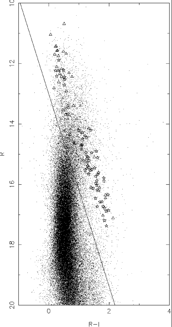
Figure 6: A colour magnitude diagram for stars in the initial sample for Alpha Per. Only stars above the line shown were included in the proper motion survey. For symbols see text.

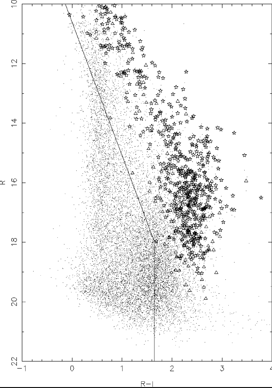
Figure 7: A colour magnitude diagram for stars in the initial sample for the Pleiades. Only stars above the line shown were included in the proper motion survey. For symbols see text.

2.5 Colour selection

After photometric recalibration, data cuts could be made on the basis of colour and brightness. Firstly it was decided that as stars brighter than $R=10$ produce high centroiding errors these would be excluded. In the Alpha Per study the low separation between the cluster and the field in the Proper Motion Vector Point Diagram produced a large amount of background star contamination at the faint end. Hence stars fainter than $R=18$ were excluded. With it’s better separation between the cluster and field such a cut was not necessary for the Pleiades data set. To reduce the amount of background star contamination colour selections were made. Figures 6 and 7 show colour magnitude diagrams for each sample. The dots represent stars in the sample while the star symbols are records from the sample which have been identified as candidates from both our study and previous studies, the triangles are star thought to be candidiates by previous studies but not by our study. It can clearly be seen that the candidate stars from other surveys form a main sequence-like line distinct from the large mass of background stars. Only stars above the line shown were used in this study. In the case of the Pleiades figure 7 shows the colour magnitude diagram. The large bulk of background stars are easily identified and removed. The line shown is again the colour cut used. Both lines used in the colour cuts were chosen by inspection As astrometric errors vary with magnitude the data was divided into the following magnitude ranges, for Alpha Per $10<R<12$, $12<R<14$, $14<R<16$ and $16<R<18$ and for the Pleiades, $10<R<12$, $12<R<14$, $14<R<16$, $16<R<17.5$ and $R>17.5$ . Each of these was treated independently in the fitting process.

2.6 The fitting process

The membership probabilities were calculated by a process similar to that outlined by Sanders (1971). The full mathematical detail is outlined in Appendix A. To ensure that the data fitting process is robust a series of twenty sets of simulated data were produced and run through the fitting program. The data sets were generated by taking uniform random number distributions. These were converted into gaussian and exponential distributions with the correct scale lengths, means and variances to model the expected distributions for the field and cluster stars. Each data set included 350 cluster stars and 350 field stars, both typical numbers for the real data. Table 3 shows the results obtained. It is apparent that there is no significant offset in any of the calculated parameter values.

Parameter	Input Value	Fitted Value
		Mean	Error
$f$	0.5	0.508	0.025
$\sigma$	3.5	3.42	0.10
$\mu_{xc}$	0.00	-0.01	0.208
$\mu_{yc}$	32.0	32.1	0.2
$\tau$	25.0	26.5	5.3
$\Sigma_{x}$	10.0	10.0	0.4
$\mu_{xf}$	0.0	-0.05	0.475

Table 3: The results of running 20 sets of simulated data through th eparameter fitting program. With the exception of $f$ all parameters have units of milliarcseconds per year.

3 Results

Figure 8: Proper motion vector point diagrams and probability histograms for each magnitude interval in the Pleiades study. In each VPD the cluster is the group in the bottom right hand corner, separate from the field stars around the origin.

Figure 9: Proper motion vector point diagrams and probability histograms for each magnitude interval in the Alpha Per study. In each VPD the cluster is the group in the bottom right hand corner, separate from the field stars around the origin.

The proper motion vector point diagrams for each of the magnitude ranges for both clusters are shown in Figure 8 (the Pleiades) and Figure 9 (Alpha Per) along with probability histograms. In the case of Alpha Per the cluster is especially apparent in the vector point diagram $16<R<18$ and consequently it also has the highest number of high probability cluster members. As the Pleiades study goes far deeper we can see the cluster becoming more apparent with increasing magnitude before becoming engulfed by the mass of field stars in the lowest magnitude interval. Accordingly the number of high probability members increases with increasing magnitude, the high number of field stars in the lowest magnitude interval means there are no stars with membership probabilities $>90\%$. A full list of stars with calculated membership probabilities greater than $60\%$ is available for both clusters from CDS in Strasbourg. Example tables are shown in Appendix B.

4 Analysis

Figure 10: An estimate of the incompleteness of the study of Alpha Per. The line shown is a least squares fit.

Figure 11: An estimate of the incompleteness of the study of the Pleiades. The line shown is a least squares fit.

Figure 12: The Luminosity Function derived for Alpha Per.

Figure 13: The Luminosity Function derived for the Pleiades. The striking feature is the peak at $R=16-17$

4.1 Luminosity Functions

As Schmidt plates have poor detection rates close to the plate limit it was necessary to carry out a completeness estimate. This was done by measuring how the number of stars in the full stellar sample increased with $R$ magnitude. For a uniform distribution of stars the number in each sample should rise exponentially with increasing magnitude with any dropoff being caused by incompleteness. An estimate of this incompleteness can be found by taking the logarithm of the number of stars in each magnitude interval, fitting a best fit line up to the point where the dropoff begins and then using the deficit to estimate the incompleteness. Figure 10 shows such a fit for the Alpha Per data set and Figure 11 that for the Pleiades sample.
The luminosity functions were found by summing the membership probabilities of stars in each one magnitude wide interval. Each interval was then corrected for incompleteness. Figure 12 shows the Luminosity Function produced for Alpha Per. Binarity was not taken into account when producing this. The luminosity function is smooth and rises with increasing magnitude. The Pleiades luminostiy function (Figure 13) by contrast has distinct features, the most obvious of which is the peak at $16<R<17$. The errors shown are Poisson errors which also take into account errors in the number of backround stars.

Figure 14: The mass-luminosity relation used for Alpha Per. The line is a sixth degree polynomial fit.

Figure 15: The mass-luminosity relation used for the Pleiades. The line is a sixth degree polynomial fit.

Figure 16: The derived cluster Mass Function for the Pleiades. Note the increasingly shallow gradient towards lower masses. The line shown is a log normal fit to the data. The solid circles are data points from this survey while the crosses are from Hambly et al (1999) and refences therein

Figure 17: The derived cluster Mass Function for Alpha Per. The line show is a power law fit.

Figure 18: A plot showing possible systematic errors in the mass luminosity relation used for the Pleiades.

Figure 19: A histogram of the membership probabilities calculated in this study of Alpha Per for stars previously identified as candidate members.

Figure 20: A histogram of the membership probabilities calculated in this study of the Pleiadesfor stars previously identified as candidate members.

4.2 Mass Function

To convert the luminosty function to a mass function a mass luminosity relationship is required. This is provided by the models of Barraffe et al (1998). Figure 14 shows the mass luminosity relation taken from these models for a 90Myr old population such as Alpha Per. The line shown is a sixth degree polynomial least squares fit to the data which is used to find the mass of a star of a particular luminosity. The mass function is found from the luminosity function, $\Phi(M)$. In some particular magnitude interval of width $dM$ there will be a number of stars $dN=\Phi(M)dM$. In the corresponding mass interval the same number $dN$ is given by $dN=\xi(m)dm$, where $dm$ is the width of the interval and $\xi(m)$ is the mass function. This can be calculated by taking the number of stars in a particular luminosity interval and dividing by the width of that interval in mass. Again binarity was not taken into account. The mass function for Alpha Per is shown in Figure 17. The mass function was then fitted by a power law fit of the form,

$$\xi(m)\propto m^{-\alpha}$$ (1)

It was found that $\alpha=0.86^{+0.14}_{-0.19}$. As mentioned earlier Barrado y Navascués’ et al (2002) derived a mass function for Alpha Per at lower masses (down to $M=0.035M_{\odot}$). They also fitted a power law function of the form, finding that $\alpha=0.59$. It therefore appears that the mass function flattens off significantly towards lower masses.
A mass function was also produced for the Pleiades. This time the mass luminosity relation was that for a 120 Myr old population and is shown in Figure 15. Again this was taken from Barraffe et al (1998). The mass function is shown in Figure 16, the data points from this survey are supplemented by those from Hambly et al (1999) and references therein. It has been suggested by Adams and Fatuzzo (1996) that the initial stellar mass function can be approximated by a log normal function as shown below,

$$log_{10}\xi(m)=a_{0}+a_{1}log_{10}m+a_{2}(log_{10}m)^{2}$$ (2)

It is clear that a power law fit is not appropriate for the mass function derived here; a log normal was fitted to the Mass function. The parameters are $a_{0}=2.213$, $a_{1}=-2.069$ and $a_{2}=-0.745$. Hambly et al (1999) produced a similar log normal fit to the mass function with parameters, $a_{0}=2.341$,$a_{1}=-2.313$ and $a_{2}=-1.191$. These are in generally good agreement with the discrepancy in $a_{2}$ probably due to the poorer constaint of the Hambly study at the faint end. The referee has pointed out the possibilty of systematic errors in the mass-luminosity relationship from the Baraffe et al (1998) models. We checked for such errors by taking an empirical $BC_{R}$ vs $T_{eff}$ relation derived using the same data and techniques as described in Hambly et al. (1999) and using it to estimate the $R$ magnitude from $M_{bol}$ for each of the points taken from Baraffe’s model. The mass of these points was then compared to that given by the mass-luminosity relation for the recalculated $R$. The results of this are shown in Figure 18.

4.3 Comparison with other studies

As mention earlier there are several other methods to determine cluster membership. Examining the membership probabilities of stars from other studies can help both to confirm individual star’s cluster membership and to examine the relevance of both study’s results. It would be worrying if candidates from previous studies did not have, by and large, high membership probabilities. The candidate stars were paired with the appropriate records in the catalogue. The maximum pairing radius was set to 6 arcseconds. A table of those candidate stars for both clusters with calculated membership probabilities is availible from CDS in Strasbourg, examples are provided in Appendix B. Figure 19 shows a histogram of the membership probabilities for these candidate stars for Alpha Per while Figure 20 shows the same graph for the Pleiades study. It is encouraging that both show that most stars thought to be members in previous studies have high membership probabilities and that the large number of probable nonmembers shown in the membership probability histograms (see Figure 8 and Figure 9) do not appear here. Both Figure 19 and Figure 20 show a sharp increase in the number of candidate stars from previous studies at p=60%. For this reason it was decided to include only stars with a membership probability greater than this in the catalogues of probable members for both clusters (available on CDS). It should be noted that several HHJ objects (see Hambly, Jameson & Hawkins 1991) do not have calculated membership probabilities. This is because these objects appeared highly elliptical on the first epoch plates SuperCOSMOS measurements and hence were not included in the present proper motion survey.

5 Conclusion

We have presented the first proper motion survey of the cluster Alpha Persei to calculate formal membership probabilities. A Luminosity Function for the range $R=10$ to $R=18$ has been produced and a Mass Fuction derived from this. The Mass Function was fitted with a power law distribution with $\alpha=0.86^{+0.14}_{-0.19}$. A catalogue of 339 high probability members has been created. This has been cross-correlated with previous studies of the cluster showing that a large number of stars previously thought to be cluster members have high calculated membership probabilities. A similar study has also been undertaken on the Pleiades and while not the first of it’s type it has produced several low mass star candidates and yielded a better constrained Mass Function at the faint end.

Appendix A Mathematics

In order to calculate membership probabilities, distributions were fitted to both the cluster stars and the field stars in the vector point diagram. The cluster stars were fitted with a circularly symmetric gaussian distribution as in Sanders (1971) however the field stars were fitted with a decaying exponential in the direction of cluster proper motion and a gaussian perpendicular to this direction as in Hambly et al (1995). In order to fit a distribution for the field stars the vector point diagram was rotated so that the cluster lay on the y axis. The total distribution function $\Phi$ is given by equation 3 where $\Phi_{f}$ is the field star distribution, $\Phi_{c}$ is the cluster star distribution and $f$ is the fraction of stars which are field stars. $\Phi_{f}$ is given in (4) and $\Phi_{c}$ is given in (5). $c_{o}$ is the normalisation for the exponential between the limits $\mu_{1}$ and $\mu_{2}$and is given by (7).

$$\Phi=f\Phi_{f}+(1-f)\Phi_{c}$$ (3)

$$\Phi_{f}=\frac{c_{o}}{\sqrt{2\pi}\Sigma_{x}}exp\left(-\frac{(\mu_{x}-\mu_{xf})^{2}}{2\Sigma_{x}^{2}}-\frac{\mu_{y}}{\tau}\right)$$ (4)

$$\Phi_{c}=\frac{1}{2\pi\sigma^{2}}exp\left(-\frac{(\mu_{x}-\mu_{xc})^{2}+(\mu_{y}-\mu_{yc})^{2}}{2\sigma^{2}}\right)$$ (5)

$$c_{o}=\frac{1}{\tau(e^{-\frac{\mu_{2}}{\tau}}-e^{-\frac{\mu_{1}}{\tau}})}$$ (6)

$$c_{o}\int_{\mu_{1}}^{\mu_{2}}e^{-\mu_{y}/\tau}d\mu_{y}=1$$ (7)

Using the maximum likelihood method

$$\sum_{i}\frac{\delta ln\Phi_{i}}{\delta\Theta}=0$$ (8)

(where $\Theta$ is some parameter) the following set of nonlinear equations are found.

$$f:\sum_{i}\frac{\Phi_{f}-\Phi_{c}}{\Phi}=0$$ (9)

$$\sigma:\sum_{i}\frac{\Phi_{c}}{\Phi}\left(\frac{(\mu_{x}-\mu_{xc})^{2}+(\mu_{y}-\mu_{yc})^{2}}{\sigma^{2}}-2\right)=0$$ (10)

$$\Sigma_{x}:\sum_{i}\frac{\Phi_{f}}{\Phi}\left(\frac{(\mu_{x}-\mu_{xf})^{2}}{\Sigma_{x}^{2}}-1\right)=0$$ (11)

$$\mu_{xf}:\sum_{i}\frac{\Phi_{f}}{\Phi}(\mu_{x}-\mu_{xf})=0$$ (12)

$$\mu_{xc}:\sum_{i}\frac{\Phi_{c}}{\Phi}(\mu_{x}-\mu_{xc})=0$$ (13)

$$\mu_{yc}:\sum_{i}\frac{\Phi_{c}}{\Phi}(\mu_{y}-\mu_{yc})=0$$ (14)

$$\tau:\sum_{i}\frac{\Phi_{f}}{\Phi}\left(\frac{\mu_{y}}{\tau}-1-c_{o}(\mu_{1}e^{-\frac{\mu_{1}}{\tau}}-\mu_{2}e^{-\frac{\mu_{2}}{\tau}})\right)=0$$ (15)

These are solved by a simple bisection algorithm. Applying the calculated values of the parameters, the probability of the ith star being a cluster member is,

$$p_{i}=\frac{(1-f)\Phi_{ci}}{\Phi_{i}}$$ (16)

The fitted values for the parameters for each magnitude interval are shown in table 4 for Alpha Per and table 5 for the Pleiades.

Interval	$f$	$\sigma$	$\mu_{xc}$	$\mu_{yc}$	$\tau$	$\Sigma_{x}$	$\mu_{xf}$
$10<R<12$	0.94	1.46	0.60	32.4	15.1	13.4	0.39
$12<R<14$	0.86	2.42	0.31	33.9	15.0	16.7	2.65
$14<R<16$	0.78	2.43	-0.07	33.9	21.8	16.2	1.54
$16<R<18$	0.76	2.96	0.72	34.6	20.3	17.1	2.165

Table 4: The calculated parameters for each magnitude interval for Alpha Per. With the exception of $f$ all parameters have units of milliarcsenonds per year.

Interval	$f$	$\sigma$	$\mu_{xc}$	$\mu_{yc}$	$\tau$	$\Sigma_{x}$	$\mu_{xf}$
$10<R<12$	0.77	3.31	-0.11	46.0	17.4	21.2	4.21
$12<R<14$	0.72	2.65	0.32	46.8	15.5	20.4	5.86
$14<R<16$	0.66	2.56	0.85	47.5	20.0	20.2	8.91
$16<R<17.5$	0.63	3.11	0.68	48.1	16.3	20.5	6.92
$R>17.5$	0.89	3.52	0.45	48.25	15.1	18.2	6.06

Table 5: The calculated parameters for each magnitude interval for the Pleiades. With the exception of $f$ all parameters have units of milliarcsenonds per year.

Appendix B Example Tables

Example Tables of the catalogue produced. All coordinates are J2000 and all magnitudes are recalibrated photographic magnitudes in the natural photographic ($R_{59F}$, $I_{IV-N}$) system. Some membership probabilities may be underestimated at the bright end due to the low separation of the main sequence from the background stars at such magnitudes in the colour magnitude diagram.

No.	RA	Dec	R	I	Membership
					Probability
1	2 51 51.84	+49 1 10.4	17.55	15.66	0.8076
2	2 52 0.93	+48 58 40.6	16.75	15.25	0.6804
3	2 53 22.99	+48 12 22.2	11.55	11.31	0.6251
4	2 53 45.30	+47 26 3.5	14.49	13.76	0.6089
5	2 54 12.10	+47 56 54.8	15.74	14.65	0.6006

Table 6: An example table of the the catalogue of high probability members of Alpha Per.

Name	Membership	No.
	Probability
HE 767	0.000001
HE 389	0.005409
AP225	0.354993
AP121	0.590439
AP102	0.000001
AP139	0.497886
AP 41	0.115724
AP118	0.007252
AP264	0.000004
AP 25	0.687682	149

Table 7: An example table of the the catalogue of candidate members of Alpha Per from other studies with calculated membership probabilities. Several of these stars have alternative names, for comprehensive cross-identifications, see the Stauffer and Prosser Catalogue of open cluster data (Stauffer, private communication).

No.	RA	Dec	R	I	Membership
					Probability
1	3 27 35.58	+24 31 43.6	12.767271	12.245660	0.926547
2	3 27 37.75	+24 59 0.8	20.631550	19.037104	0.760211
3	3 27 54.24	+24 56 11.7	16.532923	14.738454	0.943296
4	3 28 1.54	+23 4 43.0	17.342480	15.450493	0.958140
5	3 28 14.3	+26 20 35.3	13.848833	13.519602	0.639352

Table 8: An example table of the the catalogue of high probability members of the Pleiades.

Name	Membership	No.
	Probability
hcg 2	0.956371	58
hcg 6	0.933995	66
hcg 11	0.954879	92
hcg 12	0.904731	95
hcg 13	0.690341	96
hcg 16	0.906718	99

Table 9: An example table of the the catalogue of candidate members of the Pleiades from other studies with calculated membership probabilities. Several of these stars have alternative names, see the Stauffer and Prosser Catalogue of open cluster data (Stauffer, private communication).

References

(1) Adams, F.C., Fatuzzo M., ApJ, 464, 256, 1996
(2) Adams, J D., Stauffer, J R. Monet, D G., Skrutskie, M
F., Beichman, C A., AJ, 121, 2053., 2001
(3) Barrado y Navascués, D.; Bouvier, J.; Stauffer,
J. R.; Lodieu, N.; McCaughrean, M. J., A&A, 395, 813, 2002
(4) Barrado y Navascués, D., Bouvier, J., Stauffer,
J.R., Lodieu, N., MacCaughrean, M.J., Alpha Per faint stars
photometry, VizieR On-line Data Catalog: J/A+A/395/813., 2003
(6) Dobbie, P. D., Kenyon, F., Jameson, R. F., Hodgkin,
S. T., Pinfield, D. J., Osborne, S. L., MNRAS, 335, 3, 687, 2002
(7) Hambly, N.C., MacGillivray, H. T., Read, M. A.,
Tritton, S. B., Thomson, E. B., Kelly, B. D., Morgan, D. H., Smith,
R. E., Driver, S. P., Williamson, J., Parker, Q. A., Hawkins,
M. R. S., Williams, P. M., Lawrence, A., MNRAS, 326, 4,
1279, 2001
(17) Prosser, C.F., Randich, S., Simon, T.,
Identification of new low-mass members of the Alpha Persei open
cluster by ROSAT II, 1998,Astron. Nachr., 319 (1998) 4, 215
(18) Prosser, C.F., Photometry and spectroscopy in open
cluster Alpha Per, Harvard Preprint, 3761, 1993
(19) Rebolo, R., Martin, E.L., Magazzu, A., 1992,
ApJ, 389, L83-L86
(20) Sanders, W.L., 1971, A&A, 14, 226
(21) Stauffer, J.R., ApJ,, vol. 280, 189, 1984,
(22) Stauffer, J.R., Barrado Y Navascués, D., Bouier,
J., 1999,
AJ, 527, 219