Cepheid distances from infrared long-baseline interferometry

We report the angular diameter measurements of seven classical Cepheids, X Sgr, $\eta$ Aql, W Sgr, $\zeta$ Gem, $\beta$ Dor, Y Oph and $\ell$ Car that we have obtained with the VINCI instrument, installed at ESO’s VLT Interferometer (VLTI). We also present reprocessed archive data obtained with the FLUOR/IOTA instrument on $\zeta$ Gem, in order to improve the phase coverage of our observations. We obtain average limb darkened angular diameter values of $\overline{\theta_{\rm LD}}[{\rm X\,Sgr}]=1.471\pm 0.033$ mas, $\overline{\theta_{\rm LD}}[\eta\,{\rm Aql}]=1.839\pm 0.028$ mas, $\overline{\theta_{\rm LD}}[{\rm W\,Sgr}]=1.312\pm 0.029$ mas, $\overline{\theta_{\rm LD}}[\beta\,{\rm Dor}]=1.891\pm 0.024$ mas, $\overline{\theta_{\rm LD}}[\zeta\,{\rm Gem}]=1.747\pm 0.061$ mas, $\overline{\theta_{\rm LD}}[{\rm Y\,Oph}]=1.437\pm 0.040$ mas, and $\overline{\theta_{\rm LD}}[\ell\,{\rm Car}]=2.988\pm 0.012$ mas. For four of these stars, $\eta$ Aql, W Sgr, $\beta$ Dor, and $\ell$ Car, we detect the pulsational variation of their angular diameter. This enables us to compute directly their distances, using a modified version of the Baade-Wesselink method: $d[\eta\,{\rm Aql}]=276^{+55}_{-38}$ pc, $d[{\rm W\,Sgr}]=379^{+216}_{-130}$ pc, $d[\beta{\rm Dor}]=345^{+175}_{-80}$ pc, $d[\ell\,{\rm Car}]=603^{+24}_{-19}$ pc. The stated error bars are statistical in nature. Applying a hybrid method, that makes use of the Gieren et al. (gieren98 (1998)) Period-Radius relation to estimate the linear diameters, we obtain the following distances (statistical and systematic error bars are mentioned): $d[{\rm X\,Sgr}]=324\pm 7\pm 17$ pc, $d[\eta\,{\rm Aql}]=264\pm 4\pm 14$ pc, $d[{\rm W\,Sgr}]=386\pm 9\pm 21$ pc, $d[\beta{\rm Dor}]=326\pm 4\pm 19$ pc, $d[\zeta\,{\rm Gem}]=360\pm 13\pm 22$ pc, $d[{\rm Y\,Oph}]=648\pm 17\pm 47$ pc, $d[\ell\,{\rm Car}]=542\pm 2\pm 49$ pc.

1 Introduction

For almost a century, Cepheids have occupied a central role in distance determinations. This is thanks to the existence of the Period–Luminosity (P–L) relation, $M=a\,\log P+b$, which relates the logarithm of the variability period of a Cepheid to its absolute mean magnitude. These stars became even more important since the Hubble Space Telescope Key Project on the extragalactic distance scale (Freedman et al. freedman01 (2001)) has totally relied on Cepheids for the calibration of distance indicators to reach cosmologically significant distances. In other words, if the calibration of the Cepheid P–L relation is wrong, the whole extragalactic distance scale is wrong.

There are various ways to calibrate the P–L relation. The avenue chosen by the $HST$ Key-Project was to assume a distance to the Large Magellanic Cloud (LMC), thereby adopting a zero point of the distance scale. Freedman et al. (freedman01 (2001)) present an extensive discussion of all available LMC distances, and note, with other authors (see e.g. Benedict et al. benedict02 (2002)), that the LMC distance is currently the weak link in the extragalactic distance scale ladder. Another avenue is to determine the zero point of the P–L relation with Galactic Cepheids, using for instance parallax measurements, Cepheids in clusters, or through the Baade-Wesselink (BW) method. We propose in this paper and its sequels (Papers II and III) to improve the calibration of the Cepheid P–R, P–L and surface brightness–color relations through a combination of spectroscopic and interferometric observations of bright Galactic Cepheids.

In the particular case of the P–L relation, the slope $a$ is well known from Magellanic Cloud Cepheids (e.g. Udalski et al. udalski99 (1999)), though Lanoix et al. (lanoix99 (1999)) have suggested that a Malmquist effect (population incompleteness) could bias this value. On the other hand, the calibration of the zero-point $b$ (the hypothetic absolute magnitude of a 1-day period Cepheid) requires measurement of the distance to a number of nearby Cepheids with high precision. For this purpose, interferometry enables a new version of the Baade-Wesselink method, (BW, Baade baade26 (1926), Wesselink wesselink46 (1946)) for which we do not need to measure the star’s temperature, as we have directly access to its angular diameter (Davis davis79 (1979); Sasselov & Karovska sasselov94 (1994)). Using this method, we derive directly the distances to the four nearby Cepheids $\eta$ Aql, W Sgr, $\beta$ Dor and $\ell$ Car. For the remaining three objects of our sample, X Sgr, $\zeta$ Gem and Y Oph, we apply a hybrid method to derive their distances, based on published values of their linear diameters.

After a short description of the VINCI/VLTI instrument (Sect. 2), we describe the sample Cepheids that we selected (Sect. 3). In Sect. 4 and 5, we report our new observations as well as reprocessed measurements of $\zeta$ Gem retrieved from the FLUOR/IOTA instrument archive. Sect. 6 is dedicated to the computation of the corresponding angular diameter values, taking into account the limb darkening and the bandwidth smearing effects. In Sect. 7 and 8, we investigate the application of the BW method to our data, and we derive the Cepheid distances.

We will discuss the consequences of these results for the calibration of the Period-Radius (P–R), Period-Luminosity (P–L) and Barnes-Evans relations of the Cepheids in forthcoming papers (Paper II and III).

2 Instrumental setup

The European Southern Observatory’s Very Large Telescope Interferometer (Glindemann et al. glindemann (2000)) is in operation on Cerro Paranal, in Northern Chile since March 2001. For the observations reported in this paper, the beams from two Test Siderostats (0.35 m aperture) or two Unit Telescopes (8 m aperture) were recombined coherently in VINCI, the VLT INterferometer Commissioning Instrument (Kervella et al. kervella00 (2000), 2003a ). We used a regular K band filter ($\lambda=2.0-2.4\,\mu$m) that gives an effective observation wavelength of $2.18\,\mu$m for the effective temperature of typical Cepheids (see Sect. 6.4 for details). Three VLTI baselines were used for this program: E0-G1, B3-M0 and UT1-UT3 respectively 66, 140 and 102.5 m in ground length. Fig. 1 shows their positions on the VLTI platform.

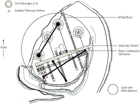
Figure 1: Layout of the three baselines used for the VINCI/VLTI Cepheids observations, UT1-UT3 (102.5 m), E0-G1 (66 m) and B3-M0 (140 m).

3 Selected sample of Cepheids

Table 1: Relevant parameters of the observed sample of Cepheids, sorted by increasing period.

	X Sgr	$\eta$ Aql	W Sgr	$\beta$ Dor	$\zeta$ Gem	Y Oph	$\ell$ Car
	HD 161592	HD 187929	HD 164975	HD 37350	HD 52973	HD 162714	HD 84810
${m_{\mathrm{V}}}^{\mathrm{a}}$	4.581	3.942	4.700	3.731	3.928	6.164	3.771
${m_{\mathrm{K}}}^{\mathrm{b}}$	2.56	1.966	2.82	1.959	2.11	2.682	1.091
Sp. Type	F5-G2II	F6Ib-G4Ib	F4-G2Ib	F4-G4Ia-II	F7Ib-G3Ib	F8Ib-G3Ib	F6Ib-K0Ib
$\pi$ (mas)c	$3.03\pm 0.94$	$2.78\pm 0.91$	$1.57\pm 0.93$	$3.14\pm 0.59$	$2.79\pm 0.81$	$1.14\pm 0.80$	$2.16\pm 0.47$
Min $\rm T_{\mathrm{eff}}$ (K)	5670	5400	5355	5025	5150
Mean $\rm T_{\mathrm{eff}}$ (K)d	6150	5870	5769	5490	5430	5300	5090
Max $\rm T_{\mathrm{eff}}$ (K)	6820	6540	6324	6090	5750
Min $\log g$	1.86	1.25	1.72	1.60
Mean $\log g^{\mathrm{e}}$	2.14	1.49	1.82	1.83	1.50	1.50	1.50
Max $\log g$	2.43	1.73	2.02	2.06
$[\mathrm{M}/\mathrm{H}]^{\mathrm{e}}$	0.04	0.05	-0.01	-0.01	0.04	0.05	0.30
$T_{0}$ (JD-$2.452.10^{6}$)f	723.9488	519.2477	726.8098	214.2153	210.7407	715.4809	290.4158
$P$ (days)g	7.013059	7.176769	7.594904	9.842425	10.150967	17.126908	35.551341
Intensity profilesh
$a_{1}$	$+0.7594$	$+0.8816$	$+0.8002$	$+0.7969$	$+0.8713$	$+0.8549$	$+0.8500$
$a_{2}$	$-0.4530$	$-0.7418$	$-0.5135$	$-0.4596$	$-0.6536$	$-0.5602$	$-0.4991$
$a_{3}$	$+0.0347$	$+0.3984$	$+0.1583$	$+0.1341$	$+0.3283$	$+0.2565$	$+0.2113$
$a_{4}$	$+0.0751$	$-0.0778$	$+0.0109$	$+0.0082$	$-0.0610$	$-0.0437$	$-0.0340$

• $m_{V}$ from Barnes et al. (barnes87 (1987)) for X Sgr, from Barnes et al. (barnes97 (1997)) for $\eta$ Aql, from Moffett & Barnes (moffett84 (1984)) for W Sgr and $\zeta$ Gem, from Berdnikov & Turner (berdnikov01 (2001)) for $\beta$ Dor and $\ell$ Car, and from Coulson & Caldwell (coulson85 (1985)) for Y Oph.

• $m_{K}$ from Welch et al. (welch84 (1984)) for X Sgr, and W Sgr, from Laney & Stobie (laney92 (1992)) for $\beta$ Dor, Y Oph, and $\ell$ Car, from Ducati et al. (ducati01 (2001)) for $\zeta$ Gem, from Barnes et al. (barnes97 (1997)) for $\eta$ Aql.

• Parallaxes from the Hipparcos catalogue (Perryman et al. hip (1997)).

• From Kiss & Szatmàry (kiss98 (1998)) for $\zeta$ Gem and $\eta$ Aql, Bersier et al. (bersier97 (1997)) for W Sgr, and Pel (pel78 (1978)) for X Sgr and $\beta$ Dor.

• From Andrievsky et al. (andrievsky02 (2002)), Cayrel de Strobel et al. (cayrel (1997), cayrel01 (2001)), and Pel (pel78 (1978)), except for $\log g$ of Y Oph.

• Reference epoch $T_{0}$ values have been computed near the dates of the VINCI observations, from the values published by Szabados (1989a ).

• $P$ values from Szabados (1989a ). The periods of $\eta$ Aql, $\zeta$ Gem and W Sgr are known to evolve. The values above correspond to the $T_{0}$ chosen for these stars.

• Four-parameters intensity profiles from Claret (claret00 (2000)) in the $K$ band, assuming a microturbulence velocity of 4 km/s and the average values of $\rm T_{\rm eff}$ and $\log g$.

Despite their brightness, Cepheids are located at large distances, and the Hipparcos satellite (Perryman et al. hip (1997)) could only obtain a limited number of Cepheid distances with a relatively poor precision. If we exclude the peculiar first overtone Cepheid $\alpha$ UMi (Polaris), the closest Cepheid is $\delta$ Cep, located at approximately 250 pc (Mourard et al. mourard97 (1997), Nordgren et al. nordgren00 (2000)). As described by Davis (davis79 (1979)) and Sasselov & Karovska (sasselov94 (1994)), it is possible to derive directly the distance to the Cepheids for which we can measure the amplitude of the angular diameter variation. Even for the nearby Cepheids, this requires an extremely high resolving power, as the largest Cepheid in the sky, $\ell$ Car, is only $0.003"$ in angular diameter. Long baseline interferometry is therefore the only technique that allows us to resolve these objects. As a remark, the medium to long period Cepheids ($D\approx 200$ D_⊙) in the Large Magellanic Cloud (LMC) ($d\approx 55$ kpc) are so small ($\theta\approx 30\,\mu$as) that they would require a baseline of 20 km to be resolved in the $K$ band (5 km in the visible). However, such a measurement is highly desirable, as it would provide a precise geometrical distance to the LMC, a critical step in the extragalactic distance ladder.

Mourard (mourard96 (1996)) has highlighted the capabilities of the VLTI for the observation of nearby Cepheids, as it provides long baselines (up to 202 m) and thus a high resolving power. Though they are supergiant stars, the Cepheids are very small objects in terms of angular size. A consequence of this is that the limit on the number of interferometrically resolvable Cepheids is not set by the size of the light collectors, but by the baseline length. From photometry only, several hundred Cepheids can produce interferometric fringes using the VLTI Auxiliary Telescopes (1.8 m in diameter). However, in order to measure accurately their size, one needs to resolve their disk to a sufficient level. Kervella (2001a ) has compiled a list of more than 30 Cepheids that can be measured from Paranal using the VINCI and AMBER (Petrov et al. petrov00 (2000)) instruments. Considering the usual constraints in terms of sky coverage, limiting magnitude and accessible resolution, we have selected seven bright Cepheids observable from Paranal Observatory (latitude $\lambda=-24\deg$): X Sgr, $\eta$ Aql, W Sgr, $\beta$ Dor, $\zeta$ Gem, Y Oph and $\ell$ Car. The periods of these stars cover a wide range, from 7 to 35.5 days. This coverage is important to properly constrain the P–R and P–L relations. To estimate the feasibility of the observations, the angular diameters of these stars were deduced from the BW studies by Gieren et al. (gieren93 (1993)). For $\zeta$ Gem and $\eta$ Aql, previously published direct interferometric measurements by Nordgren et al. (nordgren00 (2000)), Kervella et al. (2001b ) and Lane et al. (lane02 (2002)) already demonstrated the feasibility of the observations. The relevant parameters of the seven Cepheids of our sample, taken from the literature, are listed in Table 1.

4 Interferometric data processing

4.1 Coherence factors

We used a modified version (Kervella et al. 2003c ) of the standard VINCI data reduction pipeline, whose general principle is based on the original algorithm of the FLUOR instrument (Coudé du Foresto et al. cdf97 (1997), Coudé du Foresto et al. 1998a ). The VINCI/VLTI commissioning data we used for this study are publicly available through the ESO Archive, and result from two proposals of our group, that were accepted for ESO Periods 70 and 71.

The goal of the raw data processing is to extract the value of the modulated power contained in the interferometric fringes. This value is proportional to the squared visibility $V^{2}$ of the source on the observation baseline, which is in turn directly linked to the Fourier transform of the light distribution of the source through the Zernike-Van Cittert theorem.

One of the key advantages of VINCI is to use single-mode fibers to filter out the perturbations induced by the turbulent atmosphere. The wavefront that is injected in the fibers is only the mode guided by the fiber (gaussian in shape, see Ruilier ruilier99 (1999) or Coudé du Foresto 1998b for details). The atmospherically corrupted part of the wavefront is not injected into the fibers and is lost into the cladding. Due to the temporal fluctuations of the turbulence, the injected flux changes considerably during an observation. However, VINCI derives two photometric signals that can be used to subtract the intensity fluctuations from the interferometric fringes and normalize them continuously. The resulting calibrated interferograms are practically free of atmospheric corruption, except the piston mode (differential longitudinal delay of the wavefront between the two apertures) that tends to smear the fringes and affect their visibility. Its effect is largely diminished by using a sufficiently high scanning frequency, as was the case for the VINCI observations.

After the photometric calibration has been achieved, the two interferograms from the two interferometric outputs of the VINCI beam combiner are subtracted to remove the residual photometric fluctuations. As the two fringe patterns are in perfect phase opposition, this subtraction removes a large part of the correlated fluctuations and enhances the interferometric fringes. Instead of the classical Fourier analysis, we implemented a time-frequency analysis (Ségransan et al. s99 (1999)) based on the continuous wavelet transform (Farge farge92 (1992)). In this approach, the projection of the signal is not onto a sine wave (Fourier transform), but onto a function, i.e. the wavelet, that is localised in both time and frequency. We used as a basis the Morlet wavelet, a gaussian envelope multiplied by a sine wave. With the proper choice of the number of oscillations inside the gaussian envelope, this wavelet closely matches a VINCI interferogram. It is therefore very efficient at localizing the signal in both time and frequency.

The differential piston corrupts the amplitude and the shape of the fringe peak in the wavelet power spectrum. A selection based on the shape of fringe peak in the time-frequency domain is used to remove “pistonned” and false detection interferograms. Squared coherence factors $\mu^{2}$ are then derived by integrating the wavelet power spectral density (PSD) of the interferograms at the position and frequency of the fringes. The residual photon and detector noise backgrounds are removed by making a least squares fit of the PSD at high and low frequency.

4.2 Calibrators

The calibration of the Cepheids’ visibilities was achieved using well-known calibrator stars that have been selected in the Cohen et al. (cohen99 (1999)) catalogue, with the exception of $\epsilon$ Ind. This dwarf star was measured separately (Ségransan et al. segransan03 (2003)) and used to calibrate one of the $\eta$ Aql measurements. The angular diameters of 39 Eri A, HR 4050 and HR 4546 (which belong to the Cohen et al. cohen99 (1999) catalogue) were also measured separately, as these stars appeared to give a slightly inconsistent value of the interferometric efficiency.

For 39 Eri A and HR 4546, the measured angular diameters we find are $\theta_{\rm UD}=1.74\pm 0.03$ and $2.41\pm 0.04$ mas, respectively. These measured values are only $2\,\sigma$ lower than the Cohen et al (cohen99 (1999)) catalogue values of $\theta_{\rm UD}=1.81\pm 0.02$ and $2.53\pm 0.04$ mas. A possible reason for this difference could be the presence of faint, main sequence companions in orbit around these two giant stars. The additional contribution of these objects would bias the diameter found by spectrophotometry towards larger values, an effect consistent with what we observe. For HR 4050, we obtained $\theta_{\rm UD}=5.18\pm 0.05$ mas, only +1 $\sigma$ away from the catalogue value of $\theta_{\rm UD}=5.09\pm 0.06$ mas, . The characteristics of the selected calibrators are listed in Table 2. The limb-darkened disk (LD) angular diameters of these stars were converted into uniform disk values using linear coefficients taken from Claret et al. (claret95 (1995)). As demonstrated by Bordé et al. (borde (2002)), the star diameters in the Cohen et al. (cohen99 (1999)) list have been measured very homogeneously to a relative precision of approximately 1% and agree well with other angular diameter estimation methods.

The calibrators were observed soon before and after the Cepheids, in order to verify that the interferometric efficiency (IE) has not changed significantly during the Cepheid observation itself. In some cases, and due to the technical nature of commissioning observations, part of the Cepheid observations could not be bracketed, but only immediately preceded or followed by a calibrator. However, the stability of the IE has proved to be generally very good, and we do not expect any significant bias from these single-calibrator observations. Some observations included several calibrators to allow a cross-check of of their angular sizes. The calibrators were chosen as close as possible in the sky to our target Cepheids, in order to be able to observe them with similar airmass. This selection has taken into account the constraints in terms of limiting magnitude and sky coverage imposed by the VLTI siderostats and delay lines. The IE was computed from the coherence factor measurements obtained on the calibrators, taking into account the bandwidth smearing effect (see Sect. 6.4) and a uniform disk angular diameter model. This calibration process yielded the final squared visibilities listed in Tables 3 to 9.

Table 2: Relevant parameters of the calibrators.

Name		$m_{\mathrm{V}}$	$m_{\mathrm{K}}$	Sp. Type	$\rm T_{\mathrm{eff}}$(K)	$\log g$	$\pi$ (mas)a	${\theta_{\rm{LD}}}$(mas)b	${\theta_{\rm{UD}}}$(mas)c
$\chi$ Phe	HD 12524	5.16	1.52	K5III	3780	1.9	$8.76\pm 0.64$	$2.77\pm 0.032$	$2.69\pm 0.031$
39 Eri A	HD 26846	4.90	2.25	K3III	4210	2.2	$15.80\pm 0.95$	$1.79\pm 0.031^{*}$	$1.74\pm 0.030^{*}$
$\epsilon$ Ret	HD 27442	4.44	1.97	K2IVa	4460	2.3	$54.84\pm 0.50$	$1.95\pm 0.049$	$1.90\pm 0.048$
HR 2533	HD 49968	5.69	2.10	K5III	3780	1.9	$6.36\pm 0.92$	$1.93\pm 0.020$	$1.87\pm 0.019$
HR 2549	HD 50235	5.00	1.39	K5III	3780	1.9	$3.60\pm 0.56$	$2.25\pm 0.036$	$2.18\pm 0.035$
$\gamma^{2}$ Vol	HD 55865	3.77	1.52	K0III	4720	2.6	$23.02\pm 0.69$	$2.50\pm 0.060$	$2.44\pm 0.059$
6 Pup	HD 63697	5.18	2.62	K3III	4210	2.2	$12.87\pm 0.71$	$1.88\pm 0.039$	$1.83\pm 0.038$
HR 3046	HD 63744	4.70	2.31	K0III	4720	2.6	$14.36\pm 0.48$	$1.67\pm 0.025$	$1.63\pm 0.024$
HR 4050	HD 89388	3.38	0.60	K3IIa	4335	2.3	4.43 $\pm$ 0.49	$5.32\pm 0.050^{*}$	$5.18\pm 0.048^{*}$
HR 4080	HD 89998	4.83	2.40	K1III	4580	2.5	$16.26\pm 0.56$	$1.72\pm 0.020$	$1.68\pm 0.019$
HR 4526	HD 102461	5.44	1.77	K5III	3780	1.9	$3.97\pm 0.61$	$3.03\pm 0.034$	$2.94\pm 0.033$
HR 4546	HD 102964	4.47	1.56	K3III	4210	2.2	$7.03\pm 0.72$	$2.48\pm 0.036^{*}$	$2.41\pm 0.035^{*}$
HR 4831	HD 110458	4.67	2.28	K0III	4720	2.6	$17.31\pm 0.65$	$1.70\pm 0.018$	$1.66\pm 0.018$
$\chi$ Sco	HD 145897	5.25	1.60	K3III	4210	2.2	$7.43\pm 0.91$	$2.10\pm 0.023$	$2.04\pm 0.022$
70 Aql	HD 196321	4.90	1.21	K5II	3780	1.9	$1.48\pm 0.91$	$3.27\pm 0.037$	$3.17\pm 0.036$
7 Aqr	HD 199345	5.50	2.00	K5III	3780	1.9	$5.42\pm 0.99$	$2.14\pm 0.024$	$2.08\pm 0.023$
$\epsilon$ Ind	HD 209100	4.69	2.18	K4.5V	4580	4.5	$275.79\pm 0.69$	$1.89\pm 0.051^{*}$	$1.84\pm 0.050^{*}$
$\lambda$ Gru	HD 209688	4.48	1.68	K3III	4210	2.2	$13.20\pm 0.78$	$2.71\pm 0.030$	$2.64\pm 0.029$
HR 8685	HD 216149	5.41	1.60	M0III	3660	1.4	$2.95\pm 0.69$	$2.07\pm 0.021$	$2.01\pm 0.020$

• Parallaxes from the Hipparcos catalogue (Perryman et al. hip (1997)).

• Catalogue values from Cohen et al. (cohen99 (1999)), except for $\epsilon$ Ind, HR 4050 and 39 Eri A.

• Linear limb darkening coefficients factors from Claret et al. (claret95 (1995)).

• The angular diameters of $\epsilon$ Ind, HR 4050, HR 4546 and 39 Eri A have been measured separately with VINCI.

5 Data quality

5.1 General remarks

Due to the fact that we used two types of light collectors (siderostats and UTs) and several baselines (from 66 to 140 m in ground length), the intrinsic quality of our data is relatively heterogeneous. In this Section, we discuss briefly the characteristics of our observations of each target. One particularity of our measurements is that they have all been obtained during the commissioning period of the VLTI, during which technical tasks were given higher priority. In particular, the long baseline B3-M0 was only available during a few months over the two years of operations of the VLTI with VINCI. The UT1-UT3 observations were executed during two short commissioning runs and it was not possible to obtain more than one or two phases for the observed stars ($\beta$ Dor and $\zeta$ Gem). However, the very large SNR values provided by the large aperture of the UTs, even without high-order adaptive optics, gave high-precision visibility measurements.

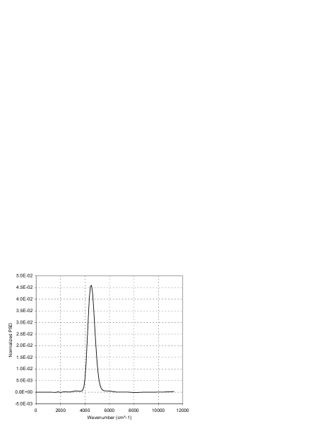
Figure 2: Average wavelets power spectral density of 302 interferograms obtained on X Sgr on JD=2452768.8462. No background or bias is present. The integration of the fringes modulated power is done between 2000 and 8000 cm^-1

The VINCI processing pipeline produces a number of outputs to the user for the data quality control, including in particular the average wavelet power spectral density (WPSD) of the processed interferograms. This is an essential tool to verify that no bias is present in the calibrated and normalized fringe power peak. Fig. 2 shows the average WPSD of a series of 302 interferograms obtained on X Sgr. No bias is present, and the residual background is very low. The power integration being done between 2000 and 8000 cm^-1, the complete modulated power of the fringes is taken into account without bias.

5.2 X Sgr, W Sgr and Y Oph

X Sgr was observed 8 times on the B3-M0 baseline (140 m ground length), using exclusively the two 0.35 m Test Siderostats (TS). The projected baseline length varied between 118.4 and 139.7 m, and the observed squared visibilities were confined between $V^{2}=56.9$ and 71.1 %. Thanks to its declination of $\delta=-28\,\deg$, X Sgr culminates almost at zenith over Paranal (-24 $\deg$), and all the observations were obtained at very low airmasses. It is located on the sky near two other Cepheids of our sample, Y Oph and W Sgr, and these three stars share the same calibrator, $\chi$ Sco. The average signal to noise ratio (SNR) was typically 2 to 5 on the photometric outputs of VINCI, and 4 to 6 on the interferometric channels, for a constant fringe frequency of 242 Hz. A total of 4 977 interferograms were processed by the pipeline. The same remarks apply to W Sgr and Y Oph, as they have almost the same magnitude and similar angular diameters. The number of processed interferograms for these two stars was 4 231 and 2 182, respectively, during 9 and 4 observing sessions.

5.3 $\eta$ Aql

$\eta$ Aql was observed once on the E0-G1 baseline (66 m) and 10 times on the B3-M0 baseline (140 m ground length). The total number of processed interferograms is 5 584. The SNRs were typically 4 and 7 on the photometric and interferometric outputs at a fringe frequency of 242 to 272 Hz. Due to its northern declination ($\delta=+1\,\deg$) and to the limits of the TS, it was not possible to observe $\eta$ Aql for more than two hours per night, therefore limiting the number of interferograms and the precision of the measurements.

5.4 $\beta$ Dor

$\beta$ Dor is a difficult target for observation with the TS, as it is partially hidden behind the TS periscopes that are used to direct the light into the VLTI tunnels. This causes a partial vignetting of the beams and therefore a loss in SNR. The data from the TS are thus of intermediate quality, considering the brightness of this star. It is located at a declination of $-62\,\deg$, relatively close to $\ell$ Car, and therefore these two stars share some calibrators. In addition to the 5 observations with the TS, four measurements were obtained during three commissioning runs on the UT1-UT3 baseline. A total of 8 129 interferograms were processed, of which 5 187 were acquired with the 8 m Unit Telescopes (96 minutes spread over four nights were spent on $\beta$ Dor using UT1 and UT3).

5.5 $\zeta$ Gem

At a declination of $+20\,\deg$, $\zeta$ Gem is not accessible to the TS due to a mechanical limitation. This is the reason why this star was observed only on two occasions with UT1 and UT3, for a total of 3 857 interferograms, obtained during 41 minutes on the target. The average on-source SNRs were typically 50 for the interferometric channels and 30 for the photometric signals, at a fringe frequency of 694 Hz.

The data obtained using the FLUOR/IOTA instrument are described in Kervella et al. (2001b ). They were reprocessed using the latest release of the FLUOR software that includes a better treatment of the photon shot noise than the 2001 version. As the baseline of IOTA is limited to 38 m, the visibility of the fringes is very high, and the precision on the angular diameter is reduced compared to the 102.5 m baseline UT1-UT3.

5.6 $\ell$ Car

As for $\beta$ Dor, the observation of $\ell$ Car ($\delta=-62\,\deg$) is made particularly difficult by the vignetting of the TS beams. Thanks to its brightness ($K\approx 1$) the SNRs are 15-20 on the interferometric channels, and 10-15 on the photometric signals, using the TS and a fringe frequency of 242 Hz. One observation was obtained on the E0-G1 baseline (66 m ground length), and 19 measurements on the B3-M0 baseline. $\ell$ Car is the most observed star in our sample, with a total of 22 226 processed interferograms. Its average diameter of approximately 3 mas makes it an ideal target for observations with baselines of 100 to 200 m. On the B3-M0 baseline, we achieved projected baselines of 89.7 to 135.0 m, corresponding to $V^{2}$ values of 8 to 42 %. This range is ideal to constrain the visibility model and derive precise values of the angular diameter.

Fig. 3 shows the squared visibility points obtained at two phases on $\ell$ Car. The change in angular diameter is clearly visible. Thanks to the variation of the projected baseline on sky, we have sampled a segment of the visibility curve.

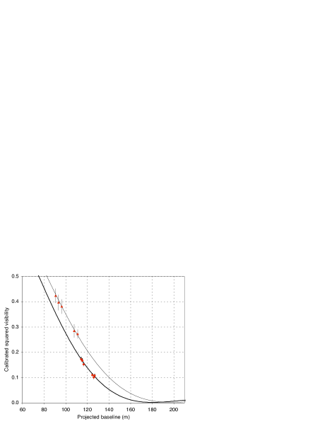
Figure 3: Squared visibilities obtained on $\ell$ Car on ${\rm JD}=2452742.712$ (thin line) and $2452763.555$ (thick line), respectively at pulsation phases 0.722 and 0.308. The two UD visibility models correspond to $\theta_{\rm UD}=2.801$ and 3.075 mas, and take the bandwidth smearing effect into account. The first minimum of the visibility function (that never goes down to zero) occurs for baselines of approximately 199 and 181 m, for an effective wavelength of $2.18\,\mu$m.

6 Angular diameters

The object of this section is to derive the angular diameters of the Cepheids as a function of their pulsational phase. We discuss the different types of models that can be used to compute the angular diameter from the squared visibility measurements.

6.1 Uniform disk angular diameters

This very simple, rather unphysical model is commonly used for interferometric studies as it is independent of any stellar atmosphere model. The relationship between the visibility $V$ and the uniform disk angular diameter (UD) is:

$$V(B,\theta_{\rm UD})=\left|\frac{2{\rm J_{1}}(x)}{x}\right|$$ (1)

where $x=\pi B\,\theta_{\rm UD}/\lambda$ is the spatial frequency. This function can be inverted numerically to retrieve the uniform disk angular diameter $\theta_{\rm UD}$.

While the true stellar light distributions depart significantly from the UD model, the UD angular diameters $\theta_{\rm UD}$ given in Tables 3 to 9 have the advantage that they can easily be converted to LD values using any stellar atmosphere model. This is achieved by computing a conversion factor $\theta_{\rm LD}/\theta_{\rm UD}$ from the chosen intensity profile (see e.g. Davis et al. davis00 (2000) for details).

6.2 Static atmosphere intensity profile

The visibility curve shape before the first minimum is almost impossible to distinguish between a uniform disk (UD) and limb darkened (LD) model. Therefore, it is necessary to use a model of the stellar disk limb darkening to deduce the photospheric angular size of the star, from the observed visibility values. The intensity profiles that we chose were computed by Claret (claret00 (2000)), based on model atmospheres by Kurucz (kurucz92 (1992)). They consist of four-parameter approximations to the function $I(\mu)/I(1)$, where $\mu=\cos\theta$ is the cosine of the azimuth of a surface element of the star. They are accurate approximations of the numerical results from the ATLAS modeling code. The analytical expression of these approximations is given by:

$${I(\mu)}/{I(1)}=1-\sum_{k=1}^{4}{a_{k}(1-\mu^{\frac{k}{2}}})$$ (2)

The $a_{k}$ coefficients are tabulated by Claret (claret00 (2000)) for a wide range of stellar parameters ($T_{\rm eff}$, $\log g$,…) and photometric bands ($U$ to $K$). The $a_{k}$ values for each Cepheid are given in Table 1 for the $K$ band, and the intensity profiles $I(\mu)/I(1)$ of X Sgr and $\ell$ Car are shown on Fig. 4.

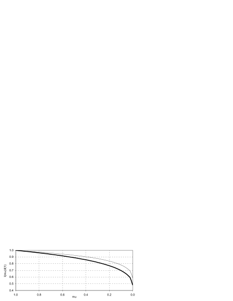
Figure 4: Average intensity profiles computed from the four-parameter approximations of Claret (claret00 (2000)) for X Sgr (thin line) and $\ell$ Car (thick line), using the parameters listed in Table 1

The limb darkening is directly measurable by interferometry around the first minimum of the visibility function, as demonstrated by several authors on giant stars (Quirrenbach et al. quirrenbach96 (1996), Wittkowski et al. wittkowski01 (2001)). Unfortunately, even for $\ell$ Car observed in the $K$ band, this requires a baseline of more than 180 m that was not available for the measurements reported here. It is intended in the near future to measure directly the LD of a few nearby Cepheids, using the shorter wavelength bands of AMBER (Petrov et al. petrov00 (2000)) and the longest baselines of the VLTI (up to 202 m).

6.3 Changes of limb darkening with phase

As shown by Marengo et al. (marengo02 (2002)), the atmosphere of the Cepheids departs from that of a non-variable giant with identical $T_{\rm eff}$ and $\log g$, due in particular to the presence of energetic shock waves at certain phases of the pulsation.

However, this effect is enhanced at visible wavelengths compared to the infrared, and appears to be negligible in the case of the VINCI observations. Marengo et al. (marengo03 (2003)) have derived in the $H$ band a relative variation of the limb darkening coefficient $k=\theta_{\rm UD}/\theta_{\rm LD}$ of only 0.2 %. This is below the precision of our measurements and is neglected in the rest of this paper. Furthermore, the VINCI/VLTI measurement wavelength being longer (2.18 $\mu$m) than the $H$ band, the LD correction is even smaller, as is its expected variation.

From the results of Marengo et al. (marengo03 (2003)) it appears clearly that the interferometers operating at infrared wavelengths are ideally suited for Cepheid measurements that aim at calibrating the P–R and P–L relations. On the other hand, as pointed out by these authors, the visible wavelength interferometers should be favored to study the dynamical evolution of the atmosphere (including the limb darkening) during the pulsation. The geometrical determination of the pulsation parallax is almost independant of the adopted atmosphere model in the $K$ band, while this is not the case at shorter wavelengths.

6.4 Visibility model and limb darkened angular diameters

The VINCI instrument bandpass corresponds to the $K$ band filter, transparent between $\lambda=2.0$ and $2.4\,\mu$m. An important effect of this relatively large spectral bandwidth is that several spatial frequencies are simultaneously observed by the interferometer. This effect is known as bandwidth smearing (Kervella et al. 2003b ).

To account for the bandwidth smearing, the model visibility is computed for regularly spaced wavenumber spectral bins over the $K$ band, and then integrated to obtain the model visibility. In this paper, we assume that the limb darkening law does not change over the $K$ band. This is reasonable for a hot and compact stellar atmosphere, but is also coherent with the range of visibilities measured on the Cepheids of our sample. If necessary, this computation can easily be extended to a wavenumber dependant $I(\mu,\sigma)$ intensity profile. Following Davis et al. (davis00 (2000)), using a Hankel integral, we can derive the visibility law $V(B,\theta_{\rm LD},\sigma)$ from the intensity profile:

$$V=\frac{1}{A}\ {\int_{0}^{1}{I(\mu)J_{0}\left({\pi B\,\sigma\,\theta_{\rm LD}\sqrt{1-\mu^{2}}}\right)}\mu\ d\mu}$$ (3)

where $\sigma$ is the wavenumber:

$$\sigma=1/\lambda$$ (4)

and $A$ is a normalization factor:

$$A={\int_{0}^{1}{I(\mu)\mu\,d\mu}}$$ (5)

The integral of the binned squared visibilities is computed numerically over the $K$ band and gives the model $V^{2}$ for the projected baseline $B$ and the angular diameter $\theta_{\rm LD}$ through the relation:

$$V^{2}(\theta_{\rm LD},B)=\int_{K}{\left[V(B,\theta_{\rm LD},\sigma)\ T(\sigma)\right]^{2}\,d\sigma}$$ (6)

where $T(\sigma)$ is the normalized instrumental transmission defined so that

$$\int_{K}T(\sigma)\,d\sigma=1$$ (7)

We computed a model of $T(\sigma)$ by taking into account the instrumental transmission of VINCI and the VLTI. It was first estimated by considering all known factors (filter, fibers, atmospheric transmission,…) and then calibrated on sky based on several observations of bright stars with the 8 meter UTs (see Kervella et al. 2003b for more details). This gives, for our sample of Cepheids, a measurement wavelength of $2.179\pm 0.003\,\mu$m. The variation of effective temperature between the stars of our sample and over the pulsation does not change this value by more than $\pm 0.001\,\mu$m. The uncertainty on the effective wavelength of the measurement translates to a 0.15 % uncertainty on the measured angular diameters. Considering the level of the other sources of error (statistical and systematic), the effect on our angular diameter results is negligible.

The $V^{2}(\theta_{\rm LD},B)$ model is adjusted numerically to the observed $(B,V^{2})$ data using a classical $\chi^{2}$ minimization process to derive $\theta_{\rm LD}$. A single angular diameter is derived per observation session, the fit being done directly on the set of $V^{2}$ values obtained during the session. The systematic and statistical errors are considered separately in the fitting procedure, to estimate the contribution of the uncertainty of the calibrator diameter on the final error bar.

Each observation session was generally executed in less than 3 hours, a short time compared to the pulsation periods of the Cepheids of our sample. Therefore, we do not expect any phase induced smearing from this averaging.

6.5 Measured angular diameters

The derived angular diameters are given in Tables 3 to 9 for the seven Cepheids of our sample. Two error bars are given for each angular diameter value:

• one statistical uncertainty, computed from the dispersion of the $V^{2}$ values obtained during the observation,

• one systematic uncertainty defined by the error bars on the calibrator stars a priori angular sizes.

While the statistical error can be diminished by repeatedly observing the target, the systematic error is not reduced by averaging measurements obtained using the same calibrator.

The reference epochs $T_{0}$ and periods $P$ for each Cepheid are given in Table 1. $N$ is the number of batches (500 interferograms) recorded during the corresponding observing session. For each angular diameter, the statistical and systematic calibration errors are given separately, except for the FLUOR/IOTA measurements of $\zeta$ Gem, for which the systematic calibration error is negligible compared to the statistical uncertainty.

Table 3: VINCI/VLTI angular diameter measurements of X Sgr.

JD	Stations	Baseline	Phase	$\theta_{\rm UD}$ (mas)	$\theta_{\rm LD}$ (mas)	$N$	$\chi^{2}_{\rm red}$	Calibrators
		(m)		$\pm$ stat. $\pm$ syst.	$\pm$ stat. $\pm$ syst.
2452741.903	B3-M0	138.366	0.560	$1.458\pm 0.048\pm 0.032$	$1.495\pm 0.049\pm 0.033$	2	0.66	$\chi$ Sco
2452742.885	B3-M0	137.432	0.700	$1.511\pm 0.058\pm 0.034$	$1.549\pm 0.059\pm 0.035$	3	0.52	$\chi$ Sco
2452743.897	B3-M0	137.903	0.844	$1.415\pm 0.055\pm 0.034$	$1.451\pm 0.057\pm 0.035$	3	0.08	$\chi$ Sco
2452744.868	B3-M0	139.657	0.983	$1.460\pm 0.051\pm 0.029$	$1.497\pm 0.052\pm 0.030$	2	0.09	$\chi$ Sco
2452747.848	B3-M0	139.530	0.408	$1.499\pm 0.213\pm 0.038$	$1.537\pm 0.219\pm 0.039$	1	-	$\chi$ Sco
2452749.832	B3-M0	139.084	0.691	$1.429\pm 0.099\pm 0.034$	$1.465\pm 0.101\pm 0.034$	2	0.35	$\chi$ Sco
2452766.811	B3-M0	138.853	0.112	$1.393\pm 0.070\pm 0.036$	$1.428\pm 0.071\pm 0.037$	4	0.09	$\chi$ Sco
2452768.877	B3-M0	128.228	0.406	$1.413\pm 0.016\pm 0.028$	$1.449\pm 0.016\pm 0.029$	6	0.62	$\chi$ Sco

Table 4: Angular diameter measurements of $\eta$ Aql.

JD	Stations	Baseline	Phase	$\theta_{\rm UD}$ (mas)	$\theta_{\rm LD}$ (mas)	$N$	$\chi^{2}_{\rm red}$	Calibrators
		(m)		$\pm$ stat. $\pm$ syst.	$\pm$ stat. $\pm$ syst.
2452524.564	E0-G1	60.664	0.741	$1.746\pm 0.100\pm 0.074$	$1.792\pm 0.103\pm 0.076$	3	0.08	70 Aql
2452557.546	B3-M0	137.625	0.336	$1.877\pm 0.098\pm 0.037$	$1.931\pm 0.101\pm 0.038$	1	-	$\epsilon$ Ind
2452559.535	B3-M0	138.353	0.614	$1.806\pm 0.037\pm 0.027$	$1.857\pm 0.038\pm 0.027$	1	-	7 Aqr, $\epsilon$ Ind
2452564.532	B3-M0	136.839	0.310	$1.809\pm 0.043\pm 0.031$	$1.860\pm 0.045\pm 0.032$	3	0.42	7 Aqr, $\epsilon$ Ind
2452565.516	B3-M0	138.495	0.447	$1.871\pm 0.017\pm 0.027$	$1.924\pm 0.017\pm 0.028$	3	0.13	7 Aqr
2452566.519	B3-M0	137.845	0.587	$1.861\pm 0.023\pm 0.026$	$1.914\pm 0.024\pm 0.026$	5	0.23	7 Aqr
2452567.523	B3-M0	137.011	0.727	$1.802\pm 0.027\pm 0.030$	$1.853\pm 0.028\pm 0.030$	2	0.62	7 Aqr
2452573.511	B3-M0	136.303	0.561	$1.884\pm 0.053\pm 0.022$	$1.938\pm 0.054\pm 0.022$	1	-	$\lambda$ Gru, HR 8685
2452769.937	B3-M0	139.632	0.931	$1.647\pm 0.026\pm 0.018$	$1.693\pm 0.026\pm 0.018$	3	0.06	$\chi$ Sco
2452770.922	B3-M0	139.400	0.068	$1.791\pm 0.041\pm 0.027$	$1.842\pm 0.042\pm 0.028$	3	0.15	$\chi$ Sco
2452772.899	B3-M0	138.188	0.343	$1.880\pm 0.044\pm 0.026$	$1.934\pm 0.046\pm 0.027$	3	0.16	7 Aqr

Table 5: Angular diameter measurements of W Sgr.

JD	Stations	Baseline	Phase	$\theta_{\rm UD}$ (mas)	$\theta_{\rm LD}$ (mas)	$N$	$\chi^{2}_{\rm red}$	Calibrators
		(m)		$\pm$ stat. $\pm$ syst.	$\pm$ stat. $\pm$ syst.
2452743.837	B3-M0	137.574	0.571	$1.408\pm 0.096\pm 0.038$	$1.447\pm 0.099\pm 0.039$	1	-	$\chi$ Sco
2452744.915	B3-M0	137.166	0.713	$1.292\pm 0.088\pm 0.034$	$1.327\pm 0.090\pm 0.035$	2	0.04	$\chi$ Sco
2452749.868	B3-M0	139.632	0.365	$1.262\pm 0.141\pm 0.040$	$1.297\pm 0.145\pm 0.041$	1	-	$\chi$ Sco
2452751.866	B3-M0	139.538	0.628	$1.320\pm 0.174\pm 0.041$	$1.357\pm 0.179\pm 0.042$	1	-	$\chi$ Sco
2452763.888	B3-M0	131.830	0.211	$1.284\pm 0.019\pm 0.029$	$1.319\pm 0.020\pm 0.030$	4	0.73	$\chi$ Sco
2452764.856	B3-M0	135.926	0.339	$1.355\pm 0.021\pm 0.021$	$1.393\pm 0.021\pm 0.022$	4	0.76	$\chi$ Sco
2452765.880	B3-M0	132.679	0.473	$1.313\pm 0.022\pm 0.025$	$1.349\pm 0.023\pm 0.026$	4	1.43	$\chi$ Sco
2452767.867	B3-M0	132.637	0.735	$1.208\pm 0.073\pm 0.039$	$1.241\pm 0.075\pm 0.040$	3	0.01	$\chi$ Sco
2452769.914	B3-M0	120.648	0.005	$1.240\pm 0.055\pm 0.034$	$1.274\pm 0.056\pm 0.035$	2	0.33	$\chi$ Sco

Table 6: Angular diameter measurements of $\beta$ Dor.

JD	Stations	Baseline	Phase	$\theta_{\rm UD}$ (mas)	$\theta_{\rm LD}$ (mas)	$N$	$\chi^{2}_{\rm red}$	Calibrators
		(m)		$\pm$ stat. $\pm$ syst.	$\pm$ stat. $\pm$ syst.
2452215.795	U1-U3	89.058	0.161	$1.842\pm 0.036\pm 0.074$	$1.896\pm 0.036\pm 0.074$	3	0.03	$\chi$ Phe, $\gamma^{2}$ Vol
2452216.785	U1-U3	89.651	0.261	$1.954\pm 0.026\pm 0.040$	$2.011\pm 0.026\pm 0.040$	7	0.10	$\gamma^{2}$ Vol
2452247.761	U1-U3	83.409	0.408	$1.921\pm 0.045\pm 0.039$	$1.977\pm 0.045\pm 0.039$	5	0.40	$\epsilon$ Ret
2452308.645	U1-U3	75.902	0.594	$1.844\pm 0.027\pm 0.071$	$1.897\pm 0.027\pm 0.071$	5	1.01	HD 63697
2452567.827	B3-M0	134.203	0.927	$1.793\pm 0.039\pm 0.049$	$1.848\pm 0.039\pm 0.049$	1	-	HR 2549
2452744.564	B3-M0	89.028	0.884	$1.730\pm 0.064\pm 0.032$	$1.780\pm 0.064\pm 0.032$	2	0.09	HR 3046, 4831
2452749.514	B3-M0	98.176	0.387	$1.921\pm 0.106\pm 0.029$	$1.978\pm 0.106\pm 0.029$	3	0.11	HR 3046
2452750.511	B3-M0	98.189	0.488	$1.864\pm 0.065\pm 0.039$	$1.919\pm 0.065\pm 0.039$	2	0.24	HR 3046
2452751.519	B3-M0	95.579	0.591	$1.954\pm 0.169\pm 0.030$	$2.012\pm 0.169\pm 0.030$	3	0.03	HR 3046

Table 7: VINCI/VLTI and FLUOR/IOTA angular diameter measurements of $\zeta$ Gem. No systematic calibration error is given for FLUOR/IOTA values (negligible compared to the statistical uncertainty). The baseline is given for the VINCI/VLTI observations (in m), while the spatial frequency (in italic) is listed for the measurements obtained with FLUOR, expressed in cycles/arcsec.

JD	Stations	B, SF	Phase	$\theta_{\rm UD}$ (mas)	$\theta_{\rm LD}$ (mas)	$N$	$\chi^{2}_{\rm red}$	Calibrators
				$\pm$ stat. $\pm$ syst.	$\pm$ stat. $\pm$ syst.
2452214.879	U1-U3	82.423	0.408	$1.677\pm 0.030\pm 0.051$	$1.725\pm 0.031\pm 0.052$	8	0.25	39 Eri
2452216.836	U1-U3	72.837	0.600	$1.712\pm 0.057\pm 0.067$	$1.760\pm 0.058\pm 0.069$	6	0.28	39 Eri, $\gamma^{2}$ Vol
2451527.972	IOTA-38m	84.870	0.739	$1.606\pm 0.334$	$1.651\pm 0.343$	1	-	HD 49968
2451601.828	IOTA-38m	83.917	0.014	$1.709\pm 0.086$	$1.795\pm 0.088$	3	0.02	HD 49968
2451259.779	IOTA-38m	83.760	0.318	$2.040\pm 0.291$	$2.144\pm 0.299$	1	-	HD 49968
2451262.740	IOTA-38m	84.015	0.610	$1.692\pm 0.273$	$1.767\pm 0.281$	2	0.13	HD 49968
2451595.863	IOTA-38m	83.790	0.427	$1.391\pm 0.284$	$1.306\pm 0.292$	2	1.72	HD 49968
2451602.764	IOTA-38m	85.010	0.107	$1.867\pm 0.216$	$1.962\pm 0.222$	2	0.02	HD 49968

Table 8: Angular diameter measurements of Y Oph.

JD	Stations	Baseline	Phase	$\theta_{\rm UD}$ (mas)	$\theta_{\rm LD}$ (mas)	$N$	$\chi^{2}_{\rm red}$	Calibrators
		(m)		$\pm$ stat. $\pm$ syst.	$\pm$ stat. $\pm$ syst.
2452742.906	B3-M0	139.569	0.601	$1.427\pm 0.115\pm 0.034$	$1.472\pm 0.119\pm 0.035$	2	0.10	$\chi$ Sco
2452750.884	B3-M0	139.057	0.067	$1.380\pm 0.100\pm 0.034$	$1.423\pm 0.103\pm 0.035$	2	0.41	$\chi$ Sco
2452772.831	B3-M0	139.657	0.349	$1.443\pm 0.051\pm 0.025$	$1.488\pm 0.053\pm 0.026$	3	0.22	$\chi$ Sco
2452782.186	B3-M0	129.518	0.168	$1.402\pm 0.027\pm 0.037$	$1.445\pm 0.028\pm 0.038$	4	0.30	$\chi$ Sco

Table 9: Angular diameter measurements of $\ell$ Car.

JD	Stations	Baseline	Phase	$\theta_{\rm UD}$ (mas)	$\theta_{\rm LD}$ (mas)	$N$	$\chi^{2}_{\rm red}$	Calibrators
		(m)		$\pm$ stat. $\pm$ syst.	$\pm$ stat. $\pm$ syst.			HR
2452453.498	E0-G1	61.069	0.587	$2.958\pm 0.039\pm 0.102$	$3.054\pm 0.041\pm 0.105$	4	0.01	4050
2452739.564	B3-M0	130.468	0.634	$2.786\pm 0.073\pm 0.042$	$2.891\pm 0.076\pm 0.043$	2	0.03	4526
2452740.569	B3-M0	128.821	0.662	$2.879\pm 0.017\pm 0.042$	$2.989\pm 0.018\pm 0.044$	7	0.77	4526
2452741.717	B3-M0	96.477	0.694	$2.893\pm 0.025\pm 0.028$	$2.993\pm 0.026\pm 0.029$	5	0.28	4526
2452742.712	B3-M0	99.848	0.722	$2.801\pm 0.034\pm 0.042$	$2.899\pm 0.035\pm 0.043$	5	0.09	4526
2452743.698	B3-M0	99.755	0.750	$2.667\pm 0.071\pm 0.015$	$2.758\pm 0.074\pm 0.016$	2	0.08	4831
2452744.634	B3-M0	114.981	0.776	$2.698\pm 0.031\pm 0.012$	$2.794\pm 0.032\pm 0.013$	6	0.73	4831
2452745.629	B3-M0	115.791	0.804	$2.584\pm 0.094\pm 0.017$	$2.675\pm 0.097\pm 0.017$	2	0.01	3046, 4546, 4831
2452746.620	B3-M0	116.828	0.832	$2.679\pm 0.023\pm 0.039$	$2.775\pm 0.023\pm 0.040$	5	0.65	3046, 4546
2452747.599	B3-M0	120.812	0.860	$2.606\pm 0.122\pm 0.025$	$2.699\pm 0.127\pm 0.026$	3	0.70	4546, 4831
2452749.576	B3-M0	124.046	0.915	$2.553\pm 0.075\pm 0.011$	$2.645\pm 0.077\pm 0.012$	4	1.18	4546
2452751.579	B3-M0	122.555	0.971	$2.657\pm 0.027\pm 0.017$	$2.753\pm 0.028\pm 0.017$	4	1.16	3046, 4831
2452755.617	B3-M0	112.185	0.085	$2.867\pm 0.109\pm 0.013$	$2.970\pm 0.113\pm 0.013$	1	-	4831
2452763.555	B3-M0	120.632	0.308	$3.077\pm 0.008\pm 0.031$	$3.194\pm 0.009\pm 0.033$	6	1.02	4546
2452765.555	B3-M0	119.629	0.365	$3.094\pm 0.011\pm 0.031$	$3.212\pm 0.011\pm 0.033$	6	1.19	4546
2452766.550	B3-M0	120.005	0.393	$3.092\pm 0.011\pm 0.032$	$3.210\pm 0.011\pm 0.033$	7	0.99	4546
2452768.566	B3-M0	115.135	0.450	$3.075\pm 0.010\pm 0.034$	$3.188\pm 0.011\pm 0.035$	7	0.46	4546
2452769.575	B3-M0	113.082	0.478	$3.075\pm 0.018\pm 0.011$	$3.189\pm 0.018\pm 0.012$	3	0.03	3046, 4831
2452770.535	B3-M0	121.152	0.505	$3.044\pm 0.019\pm 0.009$	$3.160\pm 0.020\pm 0.009$	2	0.20	3046, 4831
2452771.528	B3-M0	122.014	0.533	$3.021\pm 0.017\pm 0.010$	$3.136\pm 0.017\pm 0.010$	3	0.88	4831

7 Linear diameter curves

For each star we used radial velocity data found in the literature. Specifically, we collected data from Bersier (bersier02 (2002)) for $\eta$ Aql, $\ell$ Car, and $\beta$ Dor; from Bersier et al. (bersier94 (1994)) for $\zeta$ Gem; from Babel et al (babel89 (1989)) for W Sgr. All these data have been obtained with the CORAVEL radial velocity spectrograph (Baranne, Mayor & Poncet baranne79 (1979)). We also obtained data from Evans & Lyons (evans86 (1986)) for Y Oph and from Wilson et al. (wilson89 (1989)) for X Sgr.

In theory, the linear diameter variation could be determined by direct integration of pulsational velocities (within the assumption that the $\tau=1$ photosphere is comoving with the atmosphere of the Cepheid during its pulsation). However these velocities are deduced from the measured radial velocities by the use of a projection factor $p$. The Cepheid’s radii determined from the BW method depend directly from a good knowledge of $p$. Sabbey et al. (sabbey95 (1995)) and Krockenberger et al. (krockenberger97 (1997)) have studied in detail the way to determine the $p$-factor. We used a constant projection factor $p=1.36$ in order to transform the radial velocities into pulsation velocities. Burki et al. (burki82 (1982)) have shown that this value is appropriate for the radial velocity measurements that we used.

8 Cepheids parameters

8.1 Angular diameter model fitting and distance measurement

From our angular diameter measurements, we can derive both the average linear diameter and the distance to the Cepheids. This is done by applying a classical ${\chi}^{2}$ minimization algorithm between our angular diameter measurements and a model of the star pulsation. The minimized quantity with respect to the chosen model is

$${\chi}^{2}=\sum_{i}{\frac{(\theta_{\rm LD\,observ}(\phi_{i})-\theta_{\rm LD\,model}(\phi_{i}))^{2}}{\sigma_{\rm observ}(\phi_{i})^{2}}}$$ (8)

where $\phi_{i}$ is the phase of measurement $i$. The expression of $\theta_{\rm LD\,model}(\phi_{i})$ is defined using the following parameters:

• the average LD angular diameter $\overline{\theta_{\rm LD}}$ (in mas),

• the linear diameter variation $\Delta D(\phi_{i})$ (in $D_{\odot}$),

• the distance $d$ to the star (in pc).

The resulting expression is therefore:

$$\theta_{\rm LD\,model}(\phi_{i})=\overline{\theta_{\rm LD}}+9.305\,\left(\frac{\Delta D(\phi_{i})}{d}\right)[{\rm mas}]$$ (9)

As $\Delta D(\phi_{i})$ is known from the integration of the radial velocity curve (Sect. 7), the only variable parameters are the average LD angular diameter $\overline{\theta_{\rm LD}}$ and the distance $d$. From there, three methods can be used to derive the distance $d$, depending on the level of completeness and precision of the angular diameter measurements:

• Constant diameter fit (order 0): The average linear diameter $\overline{D}$ of the star is supposed known a priori from previously published BW measurements or P–R relations (See Sect. 8.2). We assume here that $\Delta D(\phi)=0$. The only remaining variable to fit is the distance $d$. This is the most basic method, and is useful as a reference to assess the level of detection of the pulsational diameter variation with the other methods.

• Variable diameter (order 1): We still consider that the average linear diameter $\overline{D}$ of the star is known a priori, but we include in our model the radius variation derived from the integration of the radial velocity curve. This method is well suited when the intrinsic accuracy of the angular diameter measurements is too low to measure precisely the pulsation amplitude ($\zeta$ Gem, X Sgr and Y Oph). The distance $d$ is the only free parameter for the fit.

• Complete fit (order 2): The average LD angular diameter $\overline{\theta_{\rm LD}}$ and the distance $d$ are both considered as variables and adjusted simultaneously to the angular diameter measurements. In the fitting process, the radius curve is matched to the observed pulsation amplitude. Apart from direct trigonometric parallax, this implementation of the BW method is the most direct way of measuring the distance and diameter of a Cepheid. It requires a high precision angular diameter curve and a good phase coverage. It can be applied directly to our $\eta$ Aql, W Sgr, $\beta$ Dor and $\ell$ Car measurements.

8.2 Published linear diameter values

In this section, we survey the existing linear diameter determinations for the Cepheids of our sample, in order to apply the order 0 and 1 methods to our observations.

A large number of BW studies have been published, using both visible and infrared wavelength observations. For $\zeta$ Gem and $\eta$ Aql, the pulsation has been resolved using the Palomar Testbed Interferometer (Lane et al. lane00 (2000), lane02 (2002)), thererefore giving a direct estimate of the diameter and distance of these stars. Table 10 gives a list of the existing diameter estimates for the Cepheids of our sample from the application of the classical BW method (“Baade-Wesselink” section of the table).

From the many different P–R relations available, we chose the Gieren et al. (gieren98 (1998)) version, as it is based on infrared colors for the determination of the temperature of the stars. Compared to visible colors, the infrared colors give a much less dispersed P–R relation. Indeed, this relation has a very good intrinsic precision of the order of 5 to 10 % for the period range of our sample. Moreover, it is identical to the law determined by Laney & Stobie (laney95 (1995)). The compatibility with the individual BW diameter estimates is also satisfactory. The linear diameters deduced from this P–R law are mentioned in the“Empirical P–R” section of Table 10. We assume these linear diameter values in the following.

Table 10: Published linear diameter estimates, expressed in $D_{\rm\odot}$.

	X Sgr	$\eta$ Aql	W Sgr	$\beta$ Dor	$\zeta$ Gem	Y Oph	$\ell$ Car
Interferometry
Kervella et al. (2001b )∗					$63^{+35}_{-19}$
Lane et al. (lane02 (2002))		$61.8\pm 7.6$			$66.7\pm 7.2$
Nordgren et al. (nordgren00 (2000))∗		$69^{+28}_{-15}$			$60^{+25}_{-14}$
Baade-Wesselink
Bersier et al. (bersier97 (1997))			$56.0\pm 2.9$		$89.5\pm 13.3$
Fouqué et al. (fouque03 (2003))		$48.1\pm 1.1$					$201.7\pm 3.0$
Krockenberger et al. (krockenberger97 (1997))			$56.8\pm 2.3$		$69.1^{+5.5}_{-4.8}$
Laney & Stobie (laney95 (1995))				$63.5\pm 1.8$		$92.2\pm 3.2$	$180.1\pm 4.5$
Moffett & Barnes (moffett87 (1987))a	$47.8\pm 4.5$	$52.8\pm 3.8$	$60.8\pm 7.6$		$62.6\pm 11.5$
Moffett & Barnes (moffett87 (1987))b	$49.6\pm 4.6$	$54.8\pm 3.9$	$63.1\pm 7.8$		$64.9\pm 11.9$
Sabbey et al. (sabbey95 (1995))c	$42.2\pm 4.1$	$62.7\pm 3.1$			$61.8\pm 3.5$
Sabbey et al. (sabbey95 (1995))d	$66.6\pm 4.9$	$65.8\pm 3.2$			$64.4\pm 3.6$
Sachkov et al. (sachkov98 (1998))					$74\pm 10$
Taylor et al. (taylor97 (1997))							$179.2\pm 10.4$
Taylor & Booth (taylor98 (1998))				$67.8\pm 0.7$
Turner & Burke (turner02 (2002))		$52.6\pm 8.9$		$53.8\pm 1.9$
Sasselov & Lester (sasselov90 (1990))	$67\pm 6$	$62\pm 6$
Mean B–W (overall $\sigma$)	52.5 (11.4)	59.9 (5.7)	57.0 (3.4)	65.8 (7.2)	65.3 (9.8)	92.2 (-)	180 (-)
Empirical P–R
Gieren et al. (gieren98 (1998))	$51.2\pm 2.6$	$52.1\pm 2.7$	$54.4\pm 2.9$	$66.0\pm 3.9$	$67.6\pm 4.0$	$100.1\pm 7.3$	$173.1\pm 15.8$

• $\zeta$ Gem values were derived from Kervella et al. (2001b ) and Nordgren et al. (nordgren00 (2000)) using the Hipparcos parallaxes. $\eta$ Aql was taken from Nordgren et al. (nordgren00 (2000))

• Assuming a constant $p$–factor.

• Assuming a variable $p$–factor.

• Bisector method.

• Parabolic fit method.

8.3 Angular diameter fitting results

The results of both constant and variable diameter fits for the seven Cepheids of our sample are listed in Table 11 to 13. $\eta$ Aql, W Sgr, $\beta$ Dor and $\ell$ Car gave results for all fitting methods, while X Sgr, $\zeta$ Gem and Y Oph were limited to order 1 models. For X Sgr, the order 1 fit is less adequate than the order 0, considering the quality of our measurements of this star. This is shown by the fact that the $\chi^{2}$ is significantly higher for the order 1 fit (1.36) than for the order 0 (0.38).

In the case of $\ell$ Car, the fit of a constant diameter results in a very high $\chi^{2}$ value. This means that the average diameters $\overline{\theta_{\rm UD0}}$ and $\overline{\theta_{\rm LD0}}$ should not be used for further analysis. The pulsation curve of this star is not sampled uniformly by our interferometric observations, with more values around the maximum diameter. This causes the larger diameter values to have more weight in the average diameter computation, and this produces a significant positive bias. This remark does not apply to the orders 1 and 2 fitting methods.

As a remark, no significant phase shift is detected at a level of $2.5\ 10^{-4}$ (14 minutes of time) between the predicted radius curve of $\ell$ Car and the observed angular diameter curve. The values of $P$ and $T_{0}$ used for the fit are given in Table 3.

Fig. 5 to 11 show the best models for each star, together with the VINCI/VLTI angular diameter measurements for the seven Cepheids of our sample. Fig. 12 gives an enlarged view of the maximum diameter of $\ell$ Car.

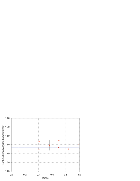
Figure 5: Order 0 model fit for X Sgr.

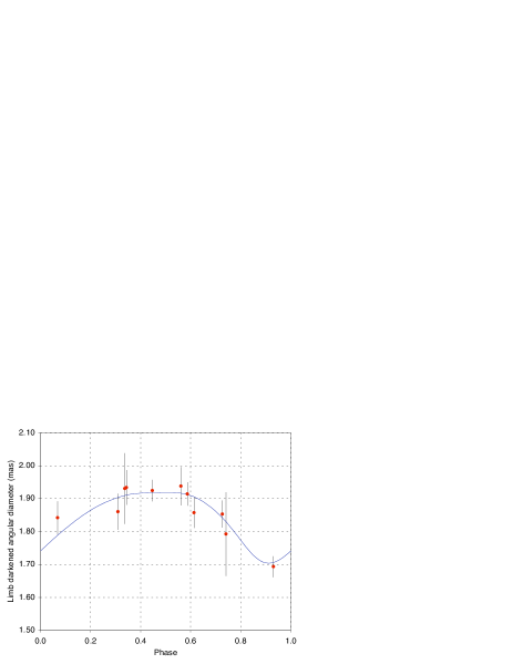
Figure 6: Order 2 model fit for $\eta$ Aql. The superimposed angular diameter variation curve (thin line) is derived from the integration of the radial velocity curve.

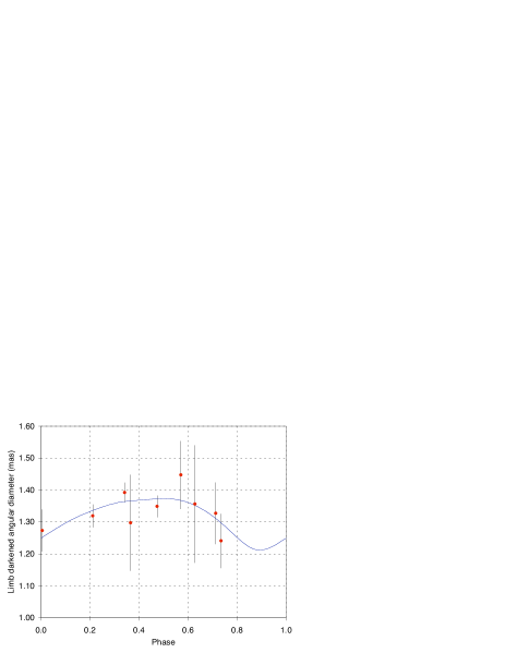
Figure 7: Order 2 model fit for W Sgr.

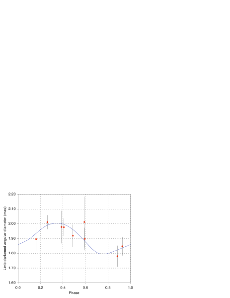
Figure 8: Order 2 model fit for $\beta$ Dor.

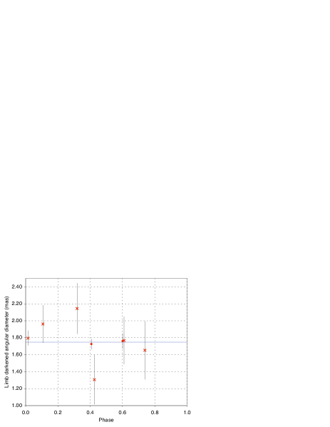
Figure 9: Order 0 model fit for $\zeta$ Gem. The crosses represent the FLUOR/IOTA data, and the two points are UT1-UT3 observations with VINCI.

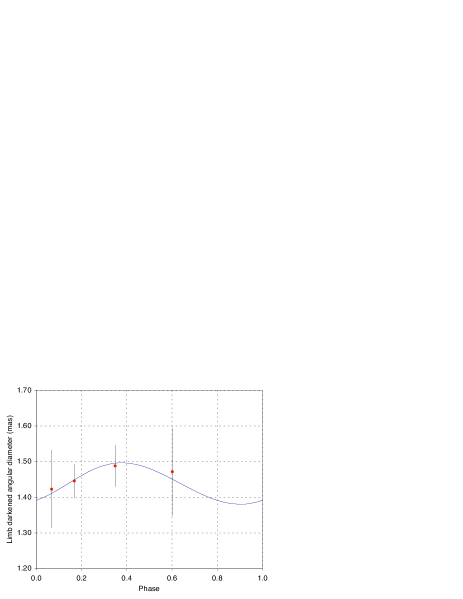
Figure 10: Order 1 model fit for Y Oph.

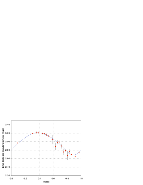
Figure 11: Order 2 model fit for $\ell$ Car.

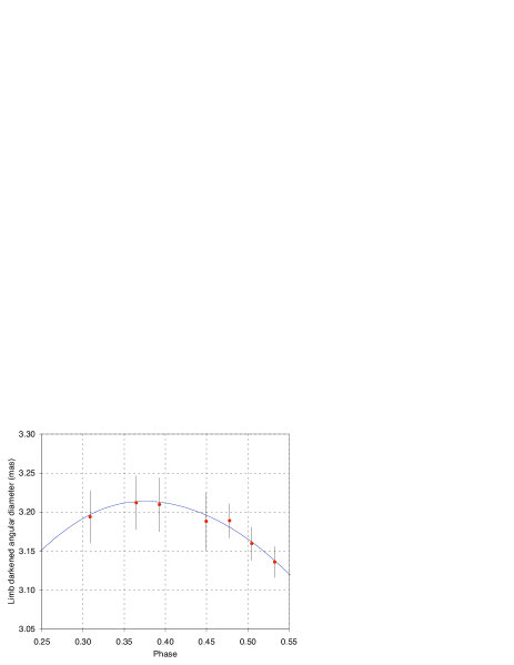
Figure 12: Detail of Fig. 11 showing the angular diameter curve of $\ell$ Car around the maximum diameter.

Table 11: Order 0. Cepheid average angular diameters and distances derived from the VINCI interferometric measurements, assuming a constant diameter model ($\Delta D=0$), The average diameter $\overline{D}$ is taken from Gieren et al. (gieren98 (1998)). Two error bars are given in brackets for the angular diameter: the statistical dispersion and the calibration systematics. The uncertainty mentioned for the distance $d$ is the quadratic sum of the statistical, calibration and P–R a priori diameter errors, the last two being systematic in nature. The three types of errors are also reported separately in brackets. The results for $\ell$ Car are mentioned only for completeness, but are not meant to be used for further analysis, as our observations are inconsistent with a constant diameter model.

Star	$\overline{\theta_{\rm LD0}}$ (mas)	$d_{0}$ (pc)	$\chi^{2}_{0}$
X Sgr	$1.471\pm 0.033_{[0.013\ 0.031]}$	$324\pm 18_{[3\ 7\ 17]}$	0.38
$\eta$ Aql	$1.856\pm 0.028_{[0.009\ 0.026]}$	$261\pm 14_{[1\ 4\ 14]}$	3.98
W Sgr	$1.348\pm 0029_{[0.011\ 0.027]}$	$376\pm 22_{[3\ 8\ 21]}$	0.90
$\beta$ Dor	$1.926\pm 0.024_{[0.014\ 0.020]}$	$319\pm 20_{[3\ 2\ 19]}$	1.31
$\zeta$ Gem	$1.747\pm 0.061_{[0.025\ 0.056]}$	$360\pm 25_{[5\ 12\ 22]}$	0.51
Y Oph	$1.459\pm 0.040_{[0.023\ 0.033]}$	$638\pm 50_{[10\ 14\ 47]}$	0.16
($\ell$ Car)	$3.071\pm 0.012_{[0.004\ 0.011]}$	$524\pm 49_{[1\ 2\ 49]}$	23.2

Table 12: Order 1. Cepheid angular diameters and distances, assuming the average diameter $\overline{D}$ of Gieren et al. (gieren98 (1998)). The diameter variation curve $\Delta D(\phi)$ is integrated from the radial velocity curve. Only the distance is ajusted by the fitting procedure. The error bars on $d$ are given as in Table 11.

Star	$\overline{\theta_{\rm LD1}}$ (mas)	$d_{1}$ (pc)	$\chi^{2}_{1}$
X Sgr	$1.461\pm 0.033_{[0.013\ 0.031]}$	$326\pm 18_{[3\ 7\ 17]}$	1.36
$\eta$ Aql	$1.839\pm 0.028_{[0.009\ 0.026]}$	$264\pm 14_{[1\ 4\ 14]}$	0.40
W Sgr	$1.312\pm 0029_{[0.011\ 0.027]}$	$386\pm 22_{[3\ 8\ 21]}$	0.42
$\beta$ Dor	$1.884\pm 0.024_{[0.014\ 0.020]}$	$326\pm 20_{[3\ 2\ 19]}$	0.23
$\zeta$ Gem	$1.718\pm 0.061_{[0.025\ 0.056]}$	$366\pm 25_{[5\ 12\ 22]}$	0.88
Y Oph	$1.437\pm 0.040_{[0.023\ 0.033]}$	$648\pm 51_{[10\ 15\ 47]}$	0.03
$\ell$ Car	$2.977\pm 0.012_{[0.004\ 0.011]}$	$542\pm 49_{[1\ 2\ 49]}$	0.71

Table 13: Order 2. Cepheid average angular diameters and distances determined through the application of the modified BW method. The only input is the diameter variation curve $\Delta D(\phi)$ derived from the integration of the radial velocity. The distance and average angular diameter are ajusted simultaneously. The statistical and systematic errors on $d$ are listed separately in brackets.

Star	$\overline{\theta_{\rm LD2}}$ (mas)	$d_{2}$ (pc)	$\chi^{2}_{2}$
$\eta$ Aql	$1.839\pm 0.028_{[0.009\ 0.026]}$	$276^{+55}_{-38}\ {[^{55\ 6}_{38\ 4}]}$	0.43
W Sgr	$1.312\pm 0.029_{[0.011\ 0.027]}$	$379^{+216}_{-130}\ {[^{216\ 11}_{130\ 7}]}$	0.48
$\beta$ Dor	$1.891\pm 0.024_{[0.014\ 0.020]}$	$345^{+175}_{-80}\ {[^{175\ 5}_{80\ 2}]}$	0.25
$\ell$ Car	$2.988\pm 0.012_{[0.004\ 0.011]}$	$603^{+24}_{-19}\ {[^{24\ 3}_{19\ 2}]}$	0.49

9 Discussion

9.1 Limb darkening of $\eta$ Aql and $\zeta$ Gem

From the NPOI (Armstrong et al. armstrong01 (2001), Nordgren et al. nordgren00 (2000)), PTI (Lane et al. lane02 (2002)) and VINCI/VLTI measurements, we know the average UD angular diameters of $\eta$ Aql and $\zeta$ Gem at several effective wavelengths with high precision. Table 14 gives the angular diameter values and the corresponding wavelengths. Claret’s (claret00 (2000)) linear limb darkening parameters $u$ were used to compute the expected conversion factors $\rho=\theta_{\rm LD}/\theta_{\rm UD}$. To read the $u$ table, we have considered the closest parameters to the average values for $\eta$ Aql and $\zeta$ Gem in Table 1, and we computed $\rho$ using the formula from Hanbury Brown el al. (hanbury74 (1974)):

$$\rho=\sqrt{\frac{1-u/3}{1-7u/15}}$$ (10)

For the NPOI observation ($\lambda_{\rm eff}\approx 0.73\,\mu$m), we have chosen an intermediate value of $u$ between the $R$ and $I$ bands.

We note that the value of $\theta_{\rm LD}$ for $\eta$ Aql that we derive for the NPOI observation, $\theta_{\rm LD}=1.73\pm 0.04$ mas, is not identical to the LD angular diameter originally given by Armstrong et al. (armstrong01 (2001)), $\theta_{\rm LD}=1.69\pm 0.04$ mas. There is a 1$\sigma$ difference, that may be due to the different source of limb darkening coefficient that these authors used for their modeling (Van Hamme vanhamme93 (1993)).

The resulting $\theta_{\rm LD}$ values for the three observations are compatible at the 2 $\sigma$ level, but there is a slight trend that points towards an underestimation of the limb darkening effect at shorter wavelengths, or alternatively its overestimation at longer wavelengths. Considering that the limb darkening is already small in the infrared, the first hypothesis seems more plausible. Marengo et al. (marengo02 (2002), marengo03 (2003)) have shown that the Cepheids limb darkening can be significantly different from stable giant stars, particularly at visible wavelengths. This could explain the observed difference between the 0.73 $\mu$m and $K$ band diameters of $\eta$ Aql and $\zeta$ Gem, the latter being probably closer to the true LD diameters, thanks to the lower limb darkening in the infrared.

In the case of $\eta$ Aql, another explanation could be that the measurement at visible wavelengths is biased by the blue companion of $\eta$ Aql. However, it is 4.6 magnitudes fainter than the Cepheid in the $V$ band (Böhm-Vitense & Proffitt bohm85 (1985), see also Sect. 9.2), and therefore should not contribute significantly to the visibility of the fringes.

Table 14: Average UD angular diameter of $\eta$ Aql and $\zeta$ Gem from the litterature, and the associated conversion factor $\rho=\theta_{\rm LD}/\theta_{\rm UD}$ from the linear limb darkening coefficients of Claret (claret00 (2000)). References: (1) Armstrong et al. (armstrong01 (2001)) and Nordgren et al. (nordgren00 (2000)), (2) Lane et al. (lane02 (2002)), (3) this work.

Ref.	$\lambda$ ($\mu$m)	$\theta_{\rm UD}$ (mas)	$\rho$	$\theta_{\rm LD}$ (mas)
$\eta$ Aql
(1)	0.73	$1.65\pm 0.04$	1.048	$1.73\pm 0.04$
(2)	1.65	$1.73\pm 0.07$	1.024	$1.77\pm 0.07$
(3)	2.18	$1.80\pm 0.03$	1.021	$1.84\pm 0.03$
$\zeta$ Gem
(1)	0.73	$1.48\pm 0.08$	1.051	$1.56\pm 0.08$
(2)	1.65	$1.61\pm 0.03$	1.027	$1.65\pm 0.03$
(3)	2.18	$1.70\pm 0.06$	1.023	$1.75\pm 0.06$

9.2 Binarity and other effects

As demonstrated by several authors (see Szabados szabados03 (2003) for a complete database), binarity and multiplicity are common in the Cepheid class. Evans (evans92a (1992)) has observed that 29 % of the Cepheids of her sample have detectable companions.

Our sample of Cepheids contains four confirmed binary Cepheids, out of a total of seven stars. As it is biased towards bright and nearby Cepheids, this large fraction is an indication that many Cepheids currently believed to be single could have undetected companions. X Sgr (Szabados 1989b ), $\eta$ Aql (Böhm-Vitense & Proffitt bohm85 (1985)), and W Sgr (Böhm-Vitense & Proffitt bohm85 (1985), Babel et al. babel89 (1989)) are confirmed members of binary or multiple systems. $\zeta$ Gem is a visual binary star (Proust et al. proust81 (1981)), but the separated companion does not contribute to our observations. Y Oph was once suspected to be a binary (Pel pel78 (1978)), but Evans (evans92a (1992)) has not confirmed the companion, and has set an upper limit of A0 on its spectral type.

The physical parameters of the companions of $\eta$ Aql and W Sgr have been derived by Böhm-Vitense & Proffitt (bohm85 (1985)) and Evans (evans91 (1991)), based on ultraviolet spectra. The latter has derived spectral types of B9.8V and A0V, respectively. The orbital parameters of the binary W Sgr were computed by Babel et al. (babel89 (1989)) and Albrow & Cottrell (albrow96 (1996)). Based on IUE spectra, Evans (evans92a (1992)) has set an upper limit of A0 on the spectral type of the companion of X Sgr.

The difference in $V$ magnitude between these three Cepheids and their companions is $\Delta{\rm M}_{V}\geq 4.5$. The $\Delta{\rm M}_{K}$ is even larger due to the blue color of these stars, $\Delta{\rm M}_{K}\geq 5.7$. Therefore, the effect on our visibility measurements is negligible, with a potential bias of $\Delta V^{2}\leq 0.5\,\%$. For example, this translates into a maximum error of $\pm 11\,\mu$as on the average angular diameter of $\eta$ Aql, (a relative error of $\pm 0.6\,\%$), that is significantly smaller than our error bars ($\pm 1.5\,\%$). In the $K$ band, the effect of the companions of the other Cepheids is also negligible at the precision level of our measurements. However, the presence of companions will have to be considered for future measurements with angular diameter precisions of a few $\mu$as. In this respect, long-period Cepheids, such as $\ell$ Car, are more reliable, as their intrinsic brightness is larger than the short-period pulsators, and therefore they dominate their potential companions even more strongly.

Fernie et al. (1995b ) have found that the amplitude of the light curve of Y Oph has been decreasing for a few decades. A similar behavior has been observed only on Polaris (e.g. Evans et al. evans02 (2002)). The uncertainty on our $\theta_{\rm LD}$ measurements has not allowed us to detect unambiguously the pulsation of this star, but it is clearly an important target for future observations using the Auxiliary Telescopes (1.8 m) of the VLTI in order to estimate its parameters with high precision.

Interestingly, Gieren et al. (gieren93 (1993)) have studied the impact of binary Cepheids on their determination of the period-luminosity relation using 100 Cepheids, and they conclude that it is negligible. This is due to the very large intrinsic luminosity of the Cepheids that overshine by several orders of magnitude most of the other types of stars.

10 Conclusion and perspectives

We have reported in this paper our long-baseline interferometric observations of seven classical Cepheids using the VINCI/VLTI instrument. For four stars ($\eta$ Aql, W Sgr, $\beta$ Dor and $\ell$ Car), we were able to apply a modified version of the BW method, resulting in an independent estimate of their distance. For all stars, we also derived their distances from lower order fitting methods, that use an a priori estimate of their linear diameter from the P–R relation of Gieren et al. (gieren98 (1998)). We would like to emphasize that the order 0/1 and order 2 error bars are different in nature, and they should be treated differently in any further use of these results. While the order 2 error bars can be treated as statistical (i.e. reduced by averaging), the order 0/1 methods errors are dominated by the systematic uncertainty introduced by the a priori estimation of the linear radius. The respective contributions of the statistical and systematic uncertainties are given separately in Tables 11 and 12. These values assume a constant value of the $p$-factor of 1.36, and can be scaled linearly for other values.

We will use these distances in Paper II, together with previously published measurements, to calibrate the zero points of the Period-Radius and Period-Luminosity relations In Paper III, we will calibrate the surface brightness–color relation, with a particular emphasis on the evolution of $\ell$ Car in this diagram over its pulsation. These three empirical relations are of critical importance for the extragalactic distance scale.

The direct measurement of the limb darkening of nearby Cepheids by interferometry is the next step of the interferometric study of these stars. It will allow a refined modeling of the atmosphere of these stars. This observation will be achieved soon using in particular the long baselines of the VLTI equipped with the AMBER instrument, and the CHARA array for the northern Cepheids. Another improvement of the interferometric BW methow will come from radial velocity measurements in the near infrared (see e.g. Butler & Bell butler97 (1997)). They will avoid any differential limb darkening between the interferometric and radial velocity measurements, and therefore make the resulting distances more immune to limb darkening uncertainties.