Astrometric Microlensing of Quasars

A small fraction of all quasars are strongly lensed and multiply imaged, with usually a galaxy acting as the main lens. Some, maybe all of these quasars are also affected by microlensing, the effects of stellar mass objects in the lensing galaxy. Stellar microlensing not only has photometric effects (the apparent magnitudes of the quasar images vary independently due to the relative motion between source, lens and observer), it also affects the observed position of the images. This astrometric effect was first explored by Lewis and Ibata (1998): the position of the quasar – i.e. the center-of-light of the many microimages – can shift by tens of microarcseconds due to the relatively sudden (dis-)appearance of a pair of microimages when a caustic is being crossed.

We explore this effect quantitatively for different values of the lensing parameters $\kappa$ and $\gamma$ (surface mass density and external shear) covering most of the known multiple quasar systems. We show examples of microlens-induced quasar motion and the corresponding light curves for different quasar sizes. We evaluate statistically the occurrence of large shifts in angular position and their correlation with apparent brightness fluctuations. We also show statistical relations between positional offsets and time from random starting points. As the amplitude of the astrometric offset depends on the source size, astrometric microlensing signatures of quasars – combined with the photometric variations – will provide very good constraints on the size of quasars as a function of wavelength. We predict that such signatures will be detectable for realistic microlensing scenarios with near future technology in the infrared/optical (Keck-Interferometry, VLTI, SIM, GAIA). Such detections will show that not even high redshift quasars define a “fixed” coordinate system.

1 Introduction

Gravitational lensing acts on quasars in a number of ways. The best known effect is strong lensing which produces multiply imaged quasars. Only a small fraction of all quasars (about 1 in 500) are multiply imaged with galaxies acting as the main lenses (for an updated list, see the CASTLES web page http://cfa-www.harvard.edu/glensdata/). Most of these quasars – and possibly some “single” quasars as well – are also affected by microlensing: the coherent effects of stellar mass objects in the lensing galaxy. Microlensing is well known for affecting the apparent brightness of the quasar, which changes due to the relative motion between lens, source and observer (see, e.g., Paczyński 1986, Wambsganss, Paczyński & Schneider 1990, Lewis et al. 1998, Wyithe et al. 2000a, Wambsganss 2001, Woźniak et al. 2000a,b). However, stellar microlensing has yet another effect, which was first explored by Lewis and Ibata (1998): when the quasar crosses a (micro-)caustic, a new pair of microimages is created or destroyed. The relatively sudden (dis-)appearance of a highly magnified image pair does not just produce a strong fluctuation in apparent brightness, it can also shift the center-of-light of the quasar (the weighted sum of all the microimages) by tens of microarcseconds. Such a positional change is in principle detectable with current VLBI techniques in the radio regime, and will be measurable in the infrared and optical wavebands as well with (near) future technology (Keck-Interferometry, VLTI, SIM, GAIA).

A number of studies have explored astrometric microlensing in a different regime, namely stars in the Milky Way (or dark matter objects in its halo) acting on background stars either in the Magellanic Clouds or in the bulge of the Milky Way (e.g., Miyamoto & Yoshii 1995; Miralda-Escude 1996; Mao & Witt 1998; Boden, Shao & van Buren 1998; Goldberg & Woźniak 1998; Paczyński 1998; Han, Chun & Chang 1999; Han & Kim 1999; Han & Jeong 1999; Safizadeh, Dalal, Griest 1999; Dominik & Sahu 2000; Gould & Han 2000; Han & Kim 2000; Salim & Gould 2000; Delplancke et al. 2001; Belokurov & Evans 2002; Dalal & Lane 2003). The effects of Milky Way stars on background quasars were studied by Hosokawa, Ohnishi & Fukushima (1997), Sazhin et al. (1998) and Honma & Kurayama (2002). Williams & Saha (1995) had discussed large image shifts produced by substructure in the lensing galaxy. However, not much work has yet been done on cosmological astrometric microlensing – stars in lensing galaxies acting on even more distant quasars – beyond Lewis & Ibata (1998), with the recent exception of Salata & Zhdanov (2003). The present paper aims to explore this further.

We study quantitatively eight different cases with various values of the surface mass density, with and without external shear. We present example microlensing lightcurves with the corresponding center-of-light shifts and we investigate the correlation between high-magnification photometric events and large-offset astrometric events.

As first pointed out by Lewis & Ibata (1998), large offset events are typically correlated with high-magnification events, whereas the inverse is much less true. The reason for this is that the location of the newly appearing bright image pair during a caustic crossing is unrelated to the previous center-of-light of the microimages. In rare cases, the new image pair may appear at or close to the center-of-light of the pre-existing microimages. Such a situation would correspond to a large change in brightness with very little change in position. In most cases, however, the new bright image pair will appear at a location which is unrelated to the previous center-of-light, and hence produce a sudden jump. Since the positional offset is preferentially perpendicular to the direction of the external shear, the shear direction can be inferred this way.

After introducing the microlensing length and time scales (Section 2), we describe our simulations (Section 3). In Section 4, we illustrate the effect of astrometric and photometric fluctuations and present statistical correlations between positional offsets, magnitude fluctuations and time intervals between the measurements for four microlensing situations with different surface mass densities ($\kappa=0.2,0.4,0.6,0.8$), with and without external shear ($\gamma=\kappa$ or 0). Finally we discuss the possibilities of real detections of this phenomenon in the near future.

2 Microlensing basics: length, time and angular scales

Table 1: Summary of scales for the “typical” lensing case ($z_{L}\approx 0.5$, $z_{Q}\approx 2$) and for the special case of Q2237+0305 ($z_{L}\approx 0.039$, $z_{Q}\approx 1.69$):

	typical lensed quasar case	lensed quasar Q2237+0305
Physical Einstein radius in quasar plane $R_{E}$	$3.2\times 10^{16}\sqrt{M/M_{\odot}}\leavevmode\nobreak\ \rm h_{75}^{-0.5}$ cm	$1.6\times 10^{16}\sqrt{M/M_{\odot}}\leavevmode\nobreak\ \rm h_{75}^{-0.5}$ cm
Angular Einstein radius $\theta_{E}$	$2.2\sqrt{M/M_{\odot}}\leavevmode\nobreak\ \rm h_{75}^{-0.5}\leavevmode\nobreak\ \mu$arcsec	$7.3\sqrt{M/M_{\odot}}\leavevmode\nobreak\ \rm h_{75}^{-0.5}\leavevmode\nobreak\ \mu$arcsec
Einstein time $t_{E}$	$25\sqrt{M/M_{\odot}}\leavevmode\nobreak\ v_{600}^{-1}\leavevmode\nobreak\ \rm h_{75}^{-0.5}$ years	$8.7\sqrt{M/M_{\odot}}\leavevmode\nobreak\ v_{600}^{-1}\leavevmode\nobreak\ \rm h_{75}^{-0.5}$ years
Crossing time $t_{cross}$	$210\leavevmode\nobreak\ R_{15}\leavevmode\nobreak\ v_{600}^{-1}\leavevmode\nobreak\ \rm h_{75}^{-0.5}$ days	$18\leavevmode\nobreak\ R_{15}\leavevmode\nobreak\ v_{600}^{-1}\leavevmode\nobreak\ \rm h_{75}^{-0.5}$ days

2.1 Standard mass, length and time scales

The lensing effects of cosmologically distant compact objects in the mass range $10^{-3}\leq M/M_{\odot}\leq 10^{3}$ on background sources is usually called “cosmological microlensing”. The source is typically a distant quasar, but in principle other objects can be microlensed as well, e.g. high-redshift supernovae (e.g., Rauch 1991) or gamma-ray sources/bursters (Torres et al. 2003; Koopmans & Wambsganss 2001). The only condition is that the source size be comparable to or smaller than the Einstein radius of the foreground lens.

The microlenses can be ordinary stars, brown dwarfs, planets, black holes, molecular clouds, or other compact mass concentrations. In most practical cases, the microlenses are part of a galaxy which acts as the main (macro-)lens. However, microlenses could also be located in, say, clusters of galaxies (Tadros, Warren & Hewett 1998, Totani 2003) or they could even be imagined “floating” freely and filling intergalactic space (Hawkins 1996, Hawkins & Taylor 1997).

The relevant length scale for microlensing is the Einstein radius in the source plane:

$$R_{E}=\sqrt{{{4GM}\over{c^{2}}}{{D_{S}D_{LS}\over D_{L}}}}\approx 3.2\times 10^{16}\sqrt{M\over M_{\odot}}\leavevmode\nobreak\ \rm h_{75}^{-0.5}\leavevmode\nobreak\ cm$$ (1)

where “typical” lens and source redshifts of $z_{L}=0.5$ and $z_{S}=2.0$ were assumed for the expression on the right hand side ($G$ and $c$ are the gravitational constant and the velocity of light, respectively; $M$ is the mass of the lens, $D_{L}$, $D_{S}$, and $D_{LS}$ are the angular diameter distances between observer – lens, observer – source, and lens – source, respectively, and a concordance cosmological model is assumed with $\Omega_{\mathrm{tot}}=1$, $\Omega_{\mathrm{matter}}=0.3$, $\Omega_{\mathrm{\Lambda}}=0.7$).

This length scale translates into an angular scale of:

$$\theta_{E}={R_{E}\over D_{S}}\approx 2.2\times 10^{-6}\sqrt{M\over M_{\odot}}\leavevmode\nobreak\ \rm h_{75}^{-0.5}\leavevmode\nobreak\ arcsec.$$ (2)

It is obvious that image splittings on such small angular scales can not be observed directly. What makes microlensing observable in the first place is the fact that observer, lens(es) and source move relative to each other. Due to this relative motion, the microimage configuration changes with time, and so does the total magnification, i.e. the combined fluxes of all the microimages which make up the macro-image. This change in magnification over time (lightcurve) can be measured: microlensing is a dynamical phenomenon.

There are two time scales involved: the standard lensing time scale $t_{E}$ is the time it takes the lens (or the source) to cross a length equivalent to the Einstein radius, i.e.

$$t_{E}=(1+z_{L}){R_{E}\over v_{\perp}}\approx 25\sqrt{M\over M_{\odot}}\leavevmode\nobreak\ v_{600}^{-1}\leavevmode\nobreak\ \rm h_{75}^{-0.5}\leavevmode\nobreak\ years,$$ (3)

where the same typical assumptions are made as above, and the relative transverse velocity $v_{600}$ is parametrized in units of $v_{\perp}=600$km/sec and for a Hubble constant $H_{0}=75h_{75}$ km/sec/Mpc. This time scale results in relatively large values. However, microlensing fluctuations are expected (and observed, see Woźniak et al. 2000a,b) on much shorter time scales. The magnification distribution is highly non-linear with sharp caustic lines separating regions of low and high magnification. Often, the density of caustics is quite high, so that a source may encounter half a dozen or more caustic lines within the length of one Einstein radius. When a source crosses a caustic, we can expect a large change in magnification (and correspondingly in position) within the time it takes the source to cross its own radius. So the relevant time scale is the “crossing time”:

$$t_{cross} = (1+z_{L}){R_{source}\over v_{\perp}(D_{S}/D_{L})}$$ (4)

$$\approx 0.58\leavevmode\nobreak\ R_{15}\leavevmode\nobreak\ v_{600}^{-1}\leavevmode\nobreak\ \rm h_{75}^{-0.5}\leavevmode\nobreak\ years$$

$$\approx 210\leavevmode\nobreak\ R_{15}\leavevmode\nobreak\ v_{600}^{-1}\leavevmode\nobreak\ \rm h_{75}^{-0.5}\leavevmode\nobreak\ days.$$

Here the quasar size $R_{15}$ is parametrized in units of $10^{15}$cm.

2.2 The special case of Q2237+0305

The quadruple quasar Q2237+0305 (Huchra et al. 1985; Irwin et al. 1989; Wambsganss et al. 1990; Wyithe et al. 2000a,b; Woźniak et al 2000a,b) is a very special and favorable case and of particular interest to microlensing studies. It was the first system in which microlensing was discovered (Irwin et al. 1989). Subsequently it received a lot of attention, both observational (Corrigan et al. 1991, Ostensen et al. 1996; Woźniak et al 2000a,b) and theoretical (Wambsganss et al. 1990; Wyithe et al. 2000a,b; Yonehara 2001). Due to the fact that the lensing galaxy is so close ($z_{G}=0.039$, Huchra et al. 1985), the physical and angular Einstein radii are considerably different from the standard case treated above:

$$r_{E,Q2237+0305}\approx 1.6\times 10^{16}\sqrt{M\over M_{\odot}}\leavevmode\nobreak\ \rm h_{75}^{-0.5}\leavevmode\nobreak\ cm,$$ (5)

$$\theta_{E,Q2237+0305}\approx 7.3\times 10^{-6}\sqrt{M\over M_{\odot}}\leavevmode\nobreak\ \rm h_{75}^{-0.5}\leavevmode\nobreak\ arcsec,$$ (6)

The resulting time scales (Einstein time and crossing time) are much shorter than in almost all other multiple quasars:

$$t_{E,Q2237+0305}\approx 8.7\sqrt{M\over M_{\odot}}\leavevmode\nobreak\ v_{600}^{-1}\leavevmode\nobreak\ \rm h_{75}^{-0.5}\leavevmode\nobreak\ years,$$ (7)

$$t_{cross,Q2237+0305}\approx 18\leavevmode\nobreak\ R_{15}\leavevmode\nobreak\ v_{600}^{-1}\leavevmode\nobreak\ \rm h_{75}^{-0.5}\leavevmode\nobreak\ days.$$ (8)

For that reason, this quadruple system is ideally suited for microlensing studies. The length, time and angular scales for the “typical case” as well as for the special case of Q2237+0305 are summarized in Table 1.

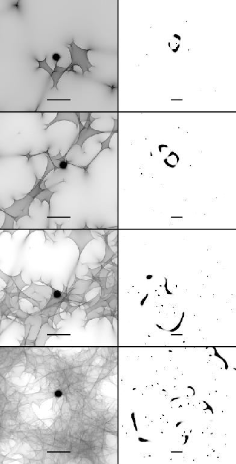
Figure 1: Illustration of source position in magnification pattern/source plane (left) and corresponding microimage configuration in the image plane, for cases $\kappa=0.2$, $\kappa=0.4$, $\kappa=0.6$, and $\kappa=0.8$ (from top to bottom) and no external shear ($\gamma=0.0$). The center-of-light position is marked with a plus sign. The horizonal bar indicates a length of two Einstein radii ($2\ R_{E}$). Note the change in scale in the right hand panels.

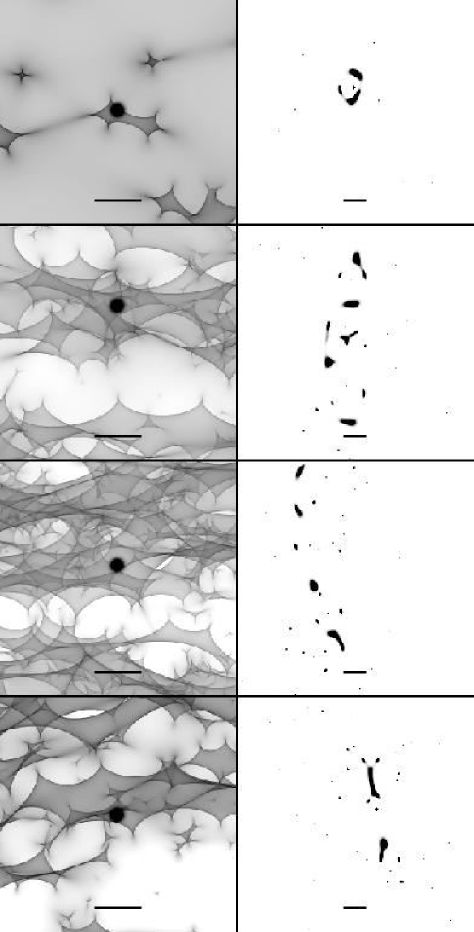
Figure 2: Same as Figure 1, here for the cases with external shear in the X-axis direction: $\kappa=\gamma=0.2$, = 0.4, = 0.6, and = 0.8 (from top to bottom); the center-of-light position is marked with a plus sign, the horizonal bar indicates a length of two Einstein radii.

3 The Simulations

In order to explore astrometric microlensing for a variety of realistic scenarios, we consider eight different cases, with the following values of the dimensionless surface mass density: $\kappa=0.2,0.4,0.6$ and 0.8. Each one of these we treated both without external shear ($\gamma=0$) and with external shear equal to the surface mass density ($\gamma=\kappa$), corresponding to an isothermal sphere model for the lensing galaxy. The shear always acts along the X-axis in the simulations. This means that the caustics are expanded in the X-direction and compressed in the Y-direction, as can be seen for example in the top left panel of Fig. 3. Horizontal bands appear on large scales (many Einstein radii). The effect is not always obvious on small scales however (sub-Einstein radii, bottom left panel of Fig. 3). Inversely, if we follow the light rays forward from source to observer (as opposed to backwards as in the simulations, which is explained below), the micro-image configuration of a source will appear compressed in the X-direction and expanded in the Y-direction (cf. the right hand panels of Fig. 3).

For each of these eight cases, we produced a magnification pattern in the source plane with a side length of $L_{A}=20\ R_{E}$, sampled on a $1000^{2}$ pixel grid, i.e. $1\ R_{E}$ is covered by 50 pixels, or $1\ {\mathrm{pix}}=0.02\ R_{E}$. This is our starting configuration A. The minimum source size we can consider is given by the pixel scale. In order to explore smaller source sizes as well (at the cost of smaller magnification patterns which may not be representative), we zoom in into the central part of the first configuration. We do higher resolution simulations (all on $1000^{2}$ pixel grids) in three steps of factors of two (configurations B, C and D, respectively), resulting in magnification patterns with side lengths of $L_{B}=10R_{E}$, $L_{C}=5R_{E}$, and $L_{D}=2.5R_{E}$, respectively. For the highest resolution simulation (configuration D), this means $R_{E}=400$ pixels, or 1 pix $=0.0025R_{E}$.

We used a modified version of the ray shooting code described in Wambsganss (1990, 1999). In the original version, rays are followed backwards from the observer through the lens plane (where all the deflections are determined) to the source plane (where the light rays are “collected” in pixels). The density of rays then indicates the magnification as a function of position in the source plane, often displayed as color coded magnification patterns. Lightcurves can be obtained by convolving a given source profile with this two-dimensional magnification map. However, all information about where the rays originated from in the lens/image plane is lost in this original algorithm. For the exploration of the centroid shift of the collection of microimages, it is exactly this information that is required. Hence we modified the code to record the positions of all the individual microimages brighter than a given magnification threshold. To do this, we defined a second, larger regular grid of $4000^{2}$ rays, which covers in the image plane a region of four times the angular side length of the magnification pattern (i.e. $(80\ \theta_{E})^{2}$ for configuration A). For a set of $1.6\times 10^{7}$ test rays, we keep track of the positions in the image plane as well as in the source plane. In this way, we can find all the positions in the image plane that are mapped onto a certain area in the source plane, and hence identify all the microimages corresponding to a particular source position and size.

In order to get information on both the magnification and the microimage locations of a finite source at a given position, we convolved the magnification pattern with a luminosity profile. We used circular sources with Gaussian widths $\sigma=$ 2, 4, 8 and 16 pixels, corresponding to physical sizes between $0.04\ R_{E}$ and $0.32\ R_{E}$ in the starting configuration A, or $1.5\times 10^{15}$cm to $1.2\times 10^{16}$cm in the typical case described in Section 2.1. We did the same with the higher resolution magnification patterns, configurations B, C and D. However, it turned out that the high resolution cases, although well suited for studying individual caustic crossings for small sources, are not quite large enough for statistical investigations. For this reason, we restricted ourselves to cases A and B for the statistical evaluations below. The numerical values corresponding to the different source sizes we used are tabulated in Table 2.

Using these simulations, we determined the positions of the individual microimages, the center-of-light and the total magnification of the macro-image corresponding to a particular source position and profile. In Figs. 1 and 2, a microimage situation is shown for each of the eight cases considered: $\kappa=0.2,0.4,0.6$ and 0.8 with $\gamma=0$ (Fig. 1), and with $\gamma=\kappa$ acting along the X-axis direction (Fig. 2). In the left columns, a small part of the magnification pattern is shown, with the source position and profile superimposed. The panels on the right hand side show the particular microimage configurations, with the light centroid indicated by a plus sign (cf. Paczyński 1986).

Table 2: Source sizes (Gaussian widths) used in our microlensing simulations (configurations A and B) in units of pixels, Einstein radii and in physical units for the typical lensed quasar and for the special case of Q2237+0305

	$\sigma$	in $R_{E}$	in cm	in cm
	in pix		(typical case)	(Q2237+0305)
A	16	0.32	$1.2\times 10^{16}$	$4\times 10^{16}$
	8	0.16	$6.0\times 10^{15}$	$2\times 10^{16}$
	4	0.08	$3.0\times 10^{15}$	$1\times 10^{16}$
	2	0.04	$1.5\times 10^{15}$	$5\times 10^{15}$
B	4	0.04	$1.5\times 10^{15}$	$5\times 10^{15}$
	2	0.02	$7.5\times 10^{14}$	$2.5\times 10^{15}$

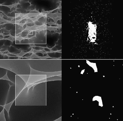
Figure 3: Illustration of the ray shooting method, here for case $\kappa=0.8$, $\gamma=0.8$. Top left: Magnification pattern in the source (quasar) plane with side length $L=10\ \theta_{E}$ (B configuration). The large square indicates the region in the source plane for which all source positions were evaluated. Top right: Corresponding microimage configuration of the large square “source” on the left, side length is 40 $\theta_{E}$: These are the parts of the sky (image plane) where light bundles originated from the square. Note the strong effect of shear in the Y-axis direction. Bottom left: The square here corresponds to the small square in the top panel, zoomed in 8 times. Bottom right: Corresponding micro-image configuration for the square on the left.

In Figure 3, the method is illustrated for $\kappa=0.8$ and $\gamma=0.8$. The top left panel shows the magnification pattern in the source (quasar) plane with side length $L=10\ \theta_{E}$ (B configuration). The grey scale indicates regions of different magnifications in the source plane: the lighter the grey, the higher magnification. The large square indicates the region in the source plane for which all source positions were evaluated. The top right panel shows the corresponding microimage configuration in the image plane: the white regions are the parts of the image plane where light bundles appear which originated from within the square on the left (side length is 40 $\theta_{E}$). In other words, it shows what a large square shaped source would look like to the observer. The bottom panels show the same for the smaller square region indicated in the top left panel, zoomed eight times. The many isolated light patches indicate that microimages are spread over a very large area in the image plane.

Figure 4 shows a quasar microlensing scenario with microlensing parameters $\kappa=0.6$ and $\gamma=0.6$, and side length 10 $\theta_{E}$ (B configuration). The straight vertical white line marks the track of the quasar motion relative to the magnification pattern; the length of the path is 2.0 $R_{E}$. For this particular track (followed from the lowest part upwards), Figure 5 shows from top to bottom: the X- and Y-coordinates of the quasar relative to the starting position ($\Delta\theta_{X}$ and $\Delta\theta_{Y}$) as a function of time; the absolute value of the positional shift ($|\Delta\theta|$) relative to the starting position as a function of time; and the corresponding light curve ($\Delta m$) of the quasar. The solid and dotted lines correspond to two different values of the source size: $\sigma=0.04R_{E}$ (4 pixels in B configuration) and $\sigma=0.16R_{E}$ (16 pixels in B configuration), respectively. The track in Fig. 4 starts in a region of low magnification which is taken as the zero point of the magnitude scale on the lowest panel in 5.

The two panels in Figure 6 represent the centroid shift for the two different source sizes. The whole track has a length of 2.0 $t_{E}$ ($\sim$ 50 and 15 years for the ’typical’ lensing case and the Q2237+0305 case, respectively). The labels $t_{0}$, $t_{1}$ and $t_{2}$ correspond to the starting, middle and final positions, respectively. Snapshots of the ensemble of microimages at times $t_{0}$, $t_{1}$ and $t_{2}$ are shown in Figure 7 assuming $\sigma=0.16R_{E}$. All microimages are plotted up to a radius of 3 $\sigma$, without accounting for the declining source profile. On average, the brightness of the macroimage declines as the fourth power of distance to the center of light (Katz, Balbus, Paczyński 1986). On our plots, due to the finite resolution, some of the distant and faint microimages appear bigger than they are. This figure simply aims at illustrating the very large spatial spread of the microimages, covering roughly $30\ \theta_{E}\times 40\ \theta_{E}$. The lower panels show enlargements of the central parts with the path of the center-of-light superimposed.

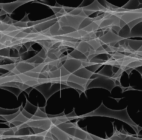
Figure 4: Illustration of a quasar microlensing scenario (here for lensing parameters $\kappa=0.6$ and $\gamma=0.6$, sidelength about 10 $R_{E}$): The gray scale indicates regions of different magnifications in the source plane. The straight vertical line marks the track of the quasar relative to the magnification pattern. The total length of the track is 2.0 $R_{E}$.

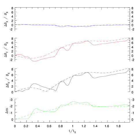
Figure 5: The four lines indicate from top to bottom: a) $\Delta\theta_{X}$, the X-coordinate of the quasar relative to the starting position as a function of time; b) same for the Y-coordinate; c) the absolute value of the positional shift $|\Delta\theta|$ relative to the starting position as a function of time; and d) the corresponding light curve of the quasar for the example track shown in Figures 4. The solid lines correspond to a source size $\sigma=0.02R_{E}$ (typically about $6.4\times 10^{14}\sqrt{M/M_{\odot}}h_{75}^{-0.5}$cm) the dashed lines to $\sigma=0.16R_{E}$ (typically about $5.1\times 10^{15}\sqrt{M/M_{\odot}}h_{75}^{-0.5}$cm).

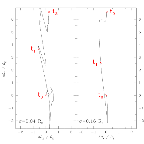
Figure 6: Effect of the source size on the centroid shift for the example track shown in Fig. 4 and 5 ($\kappa=0.6$ and $\gamma=0.6$). The two panels show the astrometric tracks that would occur for the linear quasar motion shown in Fig. 4 for two different source sizes: $\sigma=$ 0.04 and 0.16 $R_{E}$ (4 and 16 pixels in configuration B, respectively). The total length of the track is 2.0 $t_{E}$ or about 15 years for the quasar Q2237+0305. The labels $t_{0}$, $t_{1}$ and $t_{2}$ correspond to the starting, central and final positions, respectively.

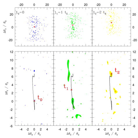
Figure 7: Top: Three snapshots of the ensemble of microimages assuming $\sigma=0.16R_{E}$. All bright microimages are plotted up to a radius of 3 $\sigma$ (due to the finite resolution of the plotting routine, some of the faint microimages are represented larger than they actually are. Left to right: starting, middle et final positions of the track in Fig. 4, corresponding to t=0.0, 1.0 and 2.0 $t_{E}$, respectively (note the angular scale: the microimage distribution covers about 30 $\theta_{E}\times\ 40\ \theta_{E}$!). Bottom: zoomed central regions; the respective positions of the center-of-light for the three epochs are marked as crosses on the track of the center-of-light (with the very central source parts corresponding to 0.5 $\sigma$ indicated in red).

4 Results and Discussion

4.1 Microlens-induced positional offsets and corresponding magnitude changes

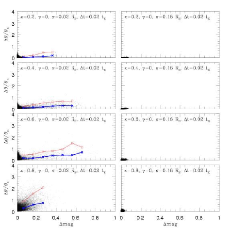
Figure 8: Offset in position $|\Delta\theta|$ versus offset in apparent brightness $|\Delta m|$, for two simulated measurements separated by $\Delta t=0.02t_{E}$. This time interval corresponds to about half a year for the “typical” lensing case and to two months for the case of Q2237+0305 (cf. Table 1). From top to bottom, the panels represent the cases $\kappa=$ 0.2, 0.4, 0.6 and 0.8, respectively, without external shear ($\gamma=0.0$). The source sizes are $\sigma=0.02R_{E}$ (left column), and $0.16R_{E}$ (right column). The median of the $|\Delta\theta|$ distribution as a function of $|\Delta m|$ is shown as a thick line (points marked as crosses), the 95th-percentile is indicated as a thin line (and squares).

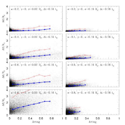
Figure 9: Same as Fig. 8, but here for two measurements separated by a larger time interval $\Delta t=0.16t_{E}$ (corresponding to about four years in the “typical” case, and 1.5 years for the case of Q2237+0305, cf. Table 1): source sizes are $\sigma=0.02R_{E}$ (left column), and $0.16R_{E}$ (right column); median of $|\Delta\theta|$ as function of $|\Delta m|$ is thick line (points are crosses), 95th-percentile is thin line (squares).

In order to evaluate the correlations between the magnitude changes and the positional changes of a microlensed quasar, we simulated pairs of measurements separated by time intervals of 0.02 $t_{E}$ (Figures 8, 10) and 0.16 $t_{E}$ (Figures 9, 11), respectively. These values correspond to about half a year and four years in the “typical” case, and to two months and 1.5 years in the case of Q2237+0305 (cf. Table 1). We placed the source at a random position in the magnification pattern and chose a second position at a distance of $0.02R_{E}$ or $0.16R_{E}$ either parallel or perpendicular to the action of the external shear (X-axis). We determined differences in the magnifications $|\Delta m|$ and the center-of-light positions $|\Delta\theta|$ between these two source positions. Each pair of measurements ($|\Delta m|$, $|\Delta\theta|$) is represented as a point in the various panels of Figures 8 to 11. In each panel, the offset in position $|\Delta\theta|$ is shown against the corresponding offset in magnitude $|\Delta m|$ for about 20,000 such measurement pairs. In the left columns of all four figures, a small Gaussian source size of $\sigma=0.02R_{E}$ is assumed, in the right column the source size is $\sigma=0.16R_{E}$. In each panel, the thick (lower) line indicates the median of $|\Delta\theta|$ as a function of $|\Delta m|$, and the thin (upper) line shows the 95th-percentile: 5% of all simulations for a given $|\Delta m|$ would result in offsets $|\Delta\theta|$ which are above this thin line.

In Figure 8, the four lensing situations without external shear are considered: $\kappa=0.2,0.4,0.6,0.8$ (from top to bottom) with a small time step $\Delta t=0.02t_{E}$. In all panels, the majority of the points cluster near the origin. This is easily understandable: the position of the source relative to the caustics has not changed by much during the short time interval, so the changes both in magnification and in the centroid position tend to be small. For small sources (left panels), however, $|\Delta m|$ and $|\Delta\theta|$ can reach relatively large values with the median lines indicating an almost linear statistical relation. The slope of these median lines slightly increases with increasing surface mass density $\kappa$. The time step corresponds roughly to the crossing time: $\Delta t=0.02t_{E}\approx t_{\mathrm{cross}}$, and there are indeed cases with easily measurable magnitude fluctuations ($|\Delta m|>0.2$ mag), which result in center-of-light offsets of about 0.5 $\theta_{E}$. In the right panel, there are no significant changes in either magnification or center-of-light position, because the source has moved only a fraction of its own diameter ($\Delta t<t_{\mathrm{cross}}$).

In Figure 9, the same is shown for a larger time step $\Delta t=0.16t_{E}$. Many more points are now spread towards larger offsets and larger magnification changes. For the small source, median values of $|\Delta\theta|\geq 1\theta_{E}$ are reached in the highest surface mass density cases. In fact, the 95th-percentile line for the $\kappa=0.8$ case indicates that for magnitude changes $|\Delta m|>0.4$mag, 5% of the all cases result in center-of-light offsets larger than 4$\theta_{E}$. For the large source (right column) the expected offsets are still quite moderate, with median values of about 0.5 $\theta_{E}$. This is not too surprising, because the time interval corresponds to just about the crossing time for the source.

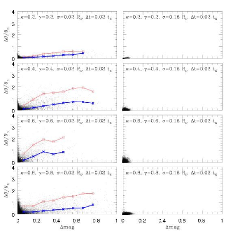
Figure 10: Same as Fig. 8, but here for the cases with external shear $\gamma=\kappa=0.2,0.4.0.6,0.8$ from top to bottom: source sizes are $\sigma=0.02R_{E}$ (left column), and $0.16R_{E}$ (right column); median of $|\Delta\theta|$ as function of $|\Delta m|$ is thick line (points are crosses), 95th-percentile is thin line (squares).

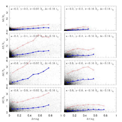
Figure 11: Same as Fig. 10, but here for the two measurements separated by a larger time interval $\Delta t=0.16t_{E}$: source sizes are $\sigma=0.02R_{E}$ (left column), and $0.16R_{E}$ (right column); median of $|\Delta\theta|$ as function of $|\Delta m|$ is thick line (points are crosses), 95th-percentile is thin line (squares).

Figures 10 and 11 contain the same diagrams for the cases with external shear, $\kappa=\gamma=0.2,0.4,0.6,0.8$ (from top to bottom). Larger offsets are reached here than in the corresponding scenarios without shear. Especially the two middle rows with $\kappa=\gamma=0.4$ and 0.6 – which best represent the typical values of convergence and shear of a multiply imaged quasar – produce values of positional offset a factor of two higher than the corresponding cases without shear: For short time steps and small sources, medians of $|\Delta\theta|\approx 1\theta_{E}$ and 95th-percentiles of $|\Delta\theta|\approx 2\theta_{E}$ (small source, left column) are reached. For smaller values of the surface mass density, the caustic density and hence the number of microimages is not large enough to produce big positional offsets, whereas for higher values of $\kappa$, the density of caustics is so high that an additional microimage pair only produces a small fluctuation.

Results are even more dramatic when assuming a larger time step ($\Delta t=0.16t_{E}$), as displayed in Figure 11: median values of $|\Delta\theta|$ between 0.5$\theta_{E}$ and 3$\theta_{E}$ for the small source size (left column), and significant median values of $|\Delta\theta|\approx 0.5\theta_{E}$ to $1\theta_{E}$ even for the large source (right column).

4.2 Microlens-induced positional offset as a function of time (with magnitude thresholds)

We evaluated the shifts in center-of-light positions for time intervals intermediate between $0.02\leq\Delta t/t_{E}\leq 0.16$ assuming a threshold for the magnitude fluctuations. In Figures 12 and 13, the median and 95th-percentile offsets are shown as a function of increasing time step $\Delta t$, for $|\Delta m|\geq 0.2$ mag (left panels) and $|\Delta m|\geq 0.5$ mag (right panels). This was done with the following idea in mind: since very accurate measurements of quasar image positions are “expensive”, it is unlikely that all lensed quasar candidates can be astrometrically monitored. However, photometric monitoring is comparably cheaper. So ideally, one could determine the positions of the most promising multiple quasars with high accuracy once, then monitor them photometrically, and whenever a large microlens-induced magnitude change has been detected, a second astrometric measurement should be performed.

In each panel of Figure 12, the two sets of curves show the median (thick lines) and the 95th-percentile (thin lines) of the $|\Delta\theta|$ distribution as a function of $\Delta t$ for the small source ($\sigma=0.02R_{E}$, solid) and the large source ($\sigma=0.16R_{E}$, dotted). All curves show basically the same behaviour: the $|\Delta\theta|$ values first increase with increasing $\Delta t$, then flatten out. This behaviour shows that many or most jumps in magnitude and position are dominated by one fold-caustic crossing. The time scale is dominated by $t_{\mathrm{cross}}$. For a slightly larger time interval, the offset does not increase significantly any more. Only for much larger $\Delta t$’s allowing for additional caustic crossings, would another increase in $|\Delta\theta|$ be expected. Offsets of more than 100 microarcseconds could indeed be reached this way, but the characteristic time scale would be depressingly large (many decades!).

The qualitative behaviour of the cases with external shear displayed in Figure 13 is similar to those without shear. However, the expected offset values are significantly higher here, as already seen in Figs. 10 and 11: again, the cases $\kappa=\gamma=0.4$ and 0.6 appear most promising (second/third row), with median values of between 1 $\theta_{E}$ and 2 $\theta_{E}$, and 95th-percentiles of 4 $\theta_{E}$ or higher. These values translate into about 7 to 15 microarcseconds (median) and $>$ 30 microarcseconds (95th percentile) when applied to the quadruple quasar Q2237+0305 (cf. Table 1). In fact, brightness fluctuations of more than one magnitude have been measured in Q2237+0305 on time scales of a few months (Woźniak 2000a,b), so these events do occur and seem not to be very rare.

4.3 Discussion and comparison with previous work

We explored astrometric microlensing effects on short timescales (of order months to years) for a set of parameter values $\kappa$ and $\gamma$. We find that the relevant time scale for measuring relatively large jumps of occasionally many tens of microarcseconds can be as short as a few months. Such sudden changes of position – produced by caustic crossings – are statistically related to fluctuations in the apparent brightness of the quasar. Therefore, a good strategy for detecting this centroid shift would be to measure the positions of the most promising lensed quasars very accurately once, then to monitor the quasars in the optical, and – when a photometric microlensing event is detected – to perform one or a few more accurate astrometric measurements.

We found that the effect is most pronounced for values of the surface mass density and shear $\kappa=\gamma=0.4$ or 0.6. These parameters happen to be applicable to many of the lensed quasar images. The most favorable case is the quadruple lens Q2237+0305: because of the closeness of the lensing galaxy, the time scale is relatively short (cf. also Woźniak 2000a,b). We also investigated the positional shift of the image as a function of source size: whereas a quasar with a typical size of $0.16\ \theta_{E}$ produces median offsets of order $\theta_{E}$ (and 95th-percentiles of about $2\ \theta_{E}$), smaller sources ($0.02\ \theta_{E}$) reach median values of $2.5\ \theta_{E}$ and 95th-percentiles larger than $5\ \theta_{E}$ (where in the case of Q2237+0305, $\theta_{E}\approx 7.3\times\sqrt{M/M_{\odot}}\leavevmode\nobreak\ \rm h_{75}^{-0.5}\leavevmode\nobreak\ \mu arcsec$, cf. Table 1).

Lewis and Ibata (1998) had investigated the astrometric microlensing effect specifically on Q2237+0305. They had found that substantial image shifts of $\approx 100\mu$arcsec are possible within months. We can confirm this in some rare cases. For typical caustic crossings with photometric fluctuations of about 0.5 mag, we find values between 20 and 40 $\mu$arcsec. Salata & Zhdanov (2003) have looked into the question of rms fluctuations of the quasar position; however, they only considered large sources ($0.5R_{E}$) and cases with $\kappa+\gamma<0.8$.

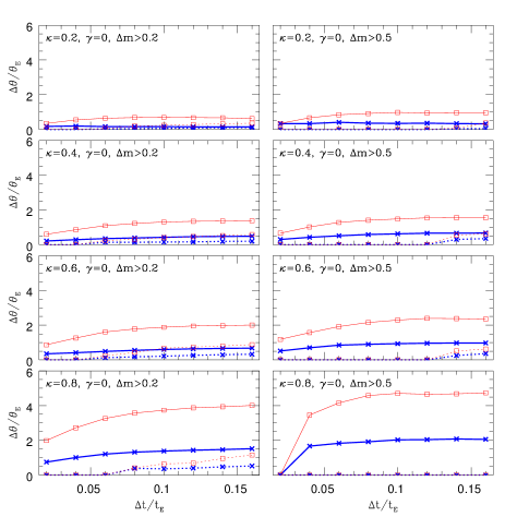
Figure 12: The median (thick lines with cross symbols) and 95th percentile (thin lines with square symbols) of the $|\Delta\theta|$ distribution as a function of $\Delta t$ for $|\Delta m|>0.2$ (left panels) and $|\Delta m|>0.5$ (right panels). The solid and dotted lines represent the two source sizes $\sigma=0.02R_{E}$ and $0.16R_{E}$, respectively. From top to bottom, the panels correspond to increasing surface mass density: $\kappa=$ 0.2, 0.4, 0.6 and 0.8, respectively, with no external shear ($\gamma=0$).

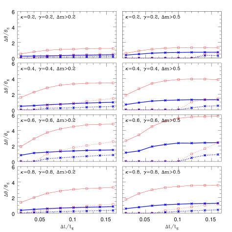
Figure 13: Same as Fig. 12, here for the cases with external shear $\gamma=\kappa=0.2,0.4,0.6,0.8$ (from top to bottom): median (thick lines, crosses) and 95th-percentile (thin lines, squares) of $|\Delta\theta|$ distribution as a function of $\Delta t$ for $|\Delta m|>0.2$ (left panels) and $|\Delta m|>0.5$ (right panels); solid lines for small source ($\sigma=0.02R_{E}$), dotted lines for large source ($0.16R_{E}$), respectively.

4.4 Prospects for observations

Ground-based differential astrometry in the near infrared is able to achieve measurement uncertainties of better than 10 microarcsec, as was reported very recently from the Palomar Testbed Interferometer (Lane & Muterspaugh 2003). This is only feasible for bright objects so far, but it is a very exciting result which opens up promising opportunities for the coming years. Another instrument promising extremely high astrometric precision in the near future (with planet detection as one of its main scientific drivers) is the PRIMA instrument at the ESO VLTI. It should become efficient in 2004 (Paresce et al. 2003; see also Delplancke et al. 2001). The current goal at ESO is to achieve 50 $\mu$arcsec accuracy with PRIMA in the $H$ and $K$ bands in 2005-2008 and 10 $\mu$arcsec accuracy in 2008-2010 (Th. Henning, private communication).

A number of space-based astrometric projects are also underway: The Space Interferometric Mission (SIM) is a five year mission scheduled for launch in 2009 (http://sim.jpl.nasa.gov). The mission’s goal is to reach an astrometric accuracy of about 1 microarcsecond for a predefined grid of objects brighter than 13 mag in the visible, which is quasi-inertially tied to a set of distant QSOs. For slightly fainter objects (the four images of the lensed quasar Q2237+0305 have magnitudes $\sim$ 17), SIM is expected to yield 4 microarcsecond absolute positions (Unwin et al. 2002). In order to detect center-of-light offsets for multiple quasars, in fact only relative astrometry between the quasar images is required. SIM will also be able to measure such positional shifts as a function of color, which will give us hints on the physical structure of the continuum emission region: presumably the cooler/redder part is more extended than the hotter/bluer part, which means that we expect larger changes in the center-of-light at shorter wavelengths. The GAIA satellite is an ESA mission currently scheduled for launch in June 2010 (see http://sci.esa.int/gaia; Perryman et al. 2001, Perryman 2002). With a nominal precision of a few microarcseconds for bright objects (about 10 microarcseconds for 15^th mag objects), it will measure accurate positions of 500 000 quasars. So GAIA is expected to be an extremely useful instrument for astrometric microlensing purposes. It will provide many positional shifts of quasar images, along with their lightcurves in many filters.

5 Summary and Conclusions

We analyzed the shifts in the center-of-light positions of gravitationaly lensed quasar images and the corresponding flux variability due to the microlensing effect of stars in the lensing galaxy. We found the following results:

1. The center-of-light of multiply imaged quasars is expected to vary on time scales of months to years, due to astrometric microlensing effects.

2. This effect depends on the size of the lensed quasar, which we modelled with a Gaussian profile: it is larger for smaller sources. This means that measuring centroid shifts will allow us to constrain the size of the quasar.

3. We studied eight cases, four without external shear ($\kappa=0.2,0.4,0.6,0.8$; $\gamma=0.0$) and four with shear ($\kappa=\gamma=0.2,0.4,0.6,0.8$). The strongest effects are seen in the cases $\kappa=\gamma=0.4$ and 0.6, which in fact are very typical parameter values for many lensed quasar images.

4. The effect of center-of-light shift of quasars is not limited to multiply imaged quasars: single quasars may occasionally be microlensed too (as was suggested by Hawkins 1996). The offsets should be relatively small, however, due to the fact that the values of $\kappa$ and $\gamma$ will be lower for single quasars than for multiply imaged ones. Our simulation with $\kappa=0.2$ comes closest to describing these cases with very low convergence.

5. The centroid shift effect is statistically strongly correlated with changes in the apparent brightness of the quasar. Both occur during the crossing of a (micro-)caustic: photometric fluctuations $\geq 0.5$ mag produce offsets $\geq 2\theta_{E}$ in 50% of the cases, and $\geq 5\theta_{E}$ in 5% of the cases. These values correspond to about 15 and 35 microarcseconds, respectively, for the lensed quasar Q2237+0305.

6. The best strategy for measuring centroid shifts is therefore to monitor the apparent brightness of multiple quasars with ground based telescopes and to determine the relative positions of the various quasar images occasionally, ideally before, during and after a high magnification event.

7. In the cases with external shear, the center-of-light shift depends strongly on the direction of the shear, which can hence be determined in a statistical sense.

With the next generation of astrometric instruments providing an accuracy of order 10 microarcseconds, the astrometric microlensing effect of stars acting on background quasars will become detectable.

References

- (1) Belokurov, V.A. & Evans, N.W.: 2002, MNRAS 341, 569
- (2) Boden, A. F., Shao, M., van Buren, D.: 1998, ApJ 502, 538
- (3) Corrigan, R.T., Irwin, M.J., Arnaud, J., Fahlman, G.G., Fletcher, J.M. et al.: 1991, AJ 102, 34
- (4) Dalal, N., Lane, B.F.: 2003, ApJ 589, 199
- (5) Delplancke, F., Górski, K.M., Richichi, A.: 2001, Astr. Astroph., 375, 701
- (6) Dominik, M., Sahu, K. C.: 2000 ApJ 524, 213
- (7) Goldberg, D. M., Woźniak, P. R.: 1998 Acta Astron. 48, 19
- GH (2000) Gould, A., Han, C. : 2000, Apj 538, 653
- (9) Han, C., Chang, K.: 1999, MNRAS 304, 845
- (10) Han, C., Chun, M.-S., Chang, K.: 1999, ApJ 526, 405
- (11) Han, C., Lee, C.: 2002, MNRAS 329, 163
- (12) Han, C., Jeong, Y.: 1999, MNRAS 309, 404
- (13) Han, C., Kim , T.-W.: 1999, MNRAS 305, 795
- HK (2) Han, C., Kim , T.-W.: 2000, ApJ 528, 687
- (15) Hawkins, M.R.S.: 1996, MNRAS 278, 787
- (16) Hawkins, M. R. S., & Taylor, A. N.: 1997, ApJ, 482, L5
- (17) Hosokawa, M., Ohnishi, K., Fukushima, T.: 1997: AJ 114, 1508
- (18) Honma, M., Kurayama, T.: 2002, ApJ 568, 717
- Huchra et al. (1985) Huchra J., Gorenstein M., Kent S., Shapiro I., Smith G., Horine E., Perley R.: 1985, AJ, 90, 691
- Irwin et al. (1989) Irwin M.J., Webster R., Hewett P.C., Corrigan R.T., Jedrzejewski R.I.: 1989, AJ, 98, 1989
- (21) Katz, N., Balbus, S., Paczyński, B.: 1986, ApJ 306, 2
- (22) Koopmans, L. V. E., Wambsganss, J.: 2001, MNRAS 325, 1317
- (23) Lane, B.F. & Muterspaugh, M.W.: 2003, preprint astro-ph/0308381
- Lewis & Ibata (1998) Lewis, G. F. & Ibata, R. A.: 1998, ApJ, 501, 478
- Lewis et al (1998) Lewis, G.F., Irwin, M.J., Hewett, P.C., Foltz, C.B.: 1998, MNRAS 295, 573
- (26) Mao, S.,Witt, H. J.: 1998 MNRAS 300, 1041
- (27) Miralda-Escude, J.: 1996, ApJ 470, L113
- (28) Miyamoto, M., Yoshii, Y.: 1995, AJ 110, 1427
- (29) Ostensen, R., Refsdal, S., Stabell, R., Teuber, J., Emanuelsen, P.I. et al.: 1996, A&A 309, 59
- P (86) Paczyński, B.: 1986, ApJ 301, 503
- P (98) Paczyński, B.: 1998, ApJ 494, L23
- (32) Paresce, F., Delplancke, F., Derie, F., Glindemann, A., Richichi, A., Tarenghi, M.: 2003, Proc. SPIE, 4838, 486
- P (01) Perryman, M.A.C., de Boer, K. S., Gilmore, G., Hog, E., Lattanzi, M. G., Lindegren, L., Luri, X., Mignard, F., Pace, O., de Zeeuw, P. T.: 2001, A&A, 369, 339
- P (02) Perryman, M.A.C.: 2002 Ap&SS, 280, 1
- R (91) Rauch, K.P.: 1991, ApJ 374, 83
- (36) Safizadeh, N., Dalal, N., Griest, K.: 1999 ApJ 522, 512
- (37) Salata, S.A., & Zhdanov, V.I.: 2003, AJ 125, 1033
- SG (2000) Salim, S., Gould, A.: 2000, Apj 539, 241
- (39) Sazhin, M.V., Zharov, V.E., Volynkin, A.V., Kalinina, T.A.: 1998, MNRAS 300, 287
- (40) Tadros, H., Warren, S., Hewett, P.: 1998, New Astr. Rev., 42, 115
- (41) Torres, D. F., Romero, G. E., Eiroa, E. F., Wambsganss, J., Pessah, M. E.: 2003, MNRAS 339, 335
- (42) Totani, T.: 2003, ApJ 586, 735
- (43) Wambsganss, J.: 1990, PhD thesis, Munich University, also available as preprint MPA 550
- (44) Wambsganss, J.: 1999, Journ. Comp. Appl. Math. 109, 353
- (45) Wambsganss, J.: 2001, Publ. Austr. Soc. Astr. 18, 207
- Wambsganss et al. (1990) Wambsganss, J., Paczyński, B., Schneider, P.: 1990, ApJL, 358, L33
- (47) Williams, L. L. R., Saha, P.: 1995, AJ 110, 1471
- (48) Woźniak, P.R., Alard, C., Udalski, A., Szymański, M., Kubiak, M., Pietrzyński, G., Zebruń, K.: 2000, ApJ 529, 88
- U (2002) Unwin, S. C., Wehrle, A. E., Jones, D. L., Meier, D. L., Piner, B. G.: 2002, PASA 19, 5
- (50) Woźniak, P.R., Udalski, A., Szymański, M., Kubiak, M., Pietrzyński, G., Soszyński, I., Zebruń, K.: 2000, ApJ 540, L65
- (51) Wyithe, J.S.B., Webster, R.L., Turner, E.L.: 2000a, MNRAS, 315, 51
- (52) Wyithe, J.S.B, Webster, R.L., Turner, E.L., Mortlock, D.J.: 2000b, MNRAS 315, 62
- (53) Yonehara, A.: 2001, ApJ, 548, L127