21 Centimeter Fluctuations from Cosmic Gas at High Redshifts

Abstract

The relatively large Thomson optical depth, $\tau_{es}$, inferred recently from the WMAP observations suggests that the Universe was reionized in a more complex manner than previously believed. However, the value of $\tau_{es}$ provides only an integral constraint on the history of reionization and, by itself, cannot be used to determine the nature of the sources responsible for this transition. Here, we show that the evolution of the ionization state of the intergalactic medium at high redshifts can be measured statistically using fluctuations in 21 centimeter radiation from neutral hydrogen. By analogy with the mathematical description of anisotropies in the cosmic microwave background, we develop a formalism to quantify the variations in 21 cm emission as a function of both frequency and angular scale. Prior to and following reionization, fluctuations in the 21 cm signal are mediated by density perturbations in the distribution of matter. Between these epochs, pockets of gas surrounding luminous objects become ionized, producing large HII regions. These “bubbles” of ionized material imprint features into the 21 cm power spectrum that make it possible to distinguish them from fluctuations produced by the density perturbations. The variation of the power spectrum with frequency can be used to infer the evolution of this process. As has been emphasized previously by others, the absolute 21 cm signal from neutral gas at high redshifts is difficult to detect owing to contamination by foreground sources. However, we argue that this source of noise can be suppressed by comparing maps closely spaced in frequency, i.e. redshift, so that 21 cm fluctuations from the IGM can be measured against a much brighter, but smoothly varying (in frequency) background.

1. Introduction

One of the long-standing goals of cosmology is to understand how structures have grown through time. In the usual paradigm, weak density perturbations were imprinted on the Universe during the inflationary era. These grew through gravitational instability, eventually forming bound halos as well as the cosmic web of sheets and filaments. Precise measurements of the cosmic microwave background (CMB) anisotropies have fixed the initial conditions of the picture (e.g., Spergel et al. 2003). The challenge now is to take structure formation beyond the well-understood linear regime in order to understand how baryons collapsed into the bound objects that we observe today, such as galaxies and galaxy clusters, and to understand how these objects affect their surroundings. At low or moderate redshifts ($z\lesssim 6$), galaxies and quasars can be studied in detail with existing technology. Unfortunately, the first generations of protogalaxies are not yet accessible observationally. Their properties are nevertheless crucial to understanding both later generations of galaxies, which form out of these early protogalaxies in any hierarchical picture of structure formation, and the gross evolution of baryons in the Universe, because these objects exhibit strong feedback on their surroundings. Perhaps the most important such channel is the reionization of the intergalactic medium (IGM). When the first protogalaxies or quasars form, they ionize pockets of surrounding gas. These H II regions grow with time and eventually overlap. The timing, morphology, and duration of this event contain a wealth of information about both the ionizing sources and the IGM (e.g., Wyithe & Loeb 2003; Cen 2003; Haiman & Holder 2003; Mackey et al. 2003; Yoshida et al. 2003a, d).

A great deal of effort has gone into constraining the transition from a neutral to ionized IGM. Unfortunately, existing observational techniques are not optimized to the needed measurements; they have provided tantalizing constraints on reionization but cannot be used to map the event in detail. The most straightforward method is to extend the “Ly$\alpha$ forest” to high redshifts: regions with relatively large H I densities appear as absorption troughs in quasar spectra, which presumably deepen and come to dominate the spectra as we approach the reionization epoch. Indeed, spectra of $z\sim 6$ quasars selected from the Sloan Digital Sky Survey (SDSS) show at least one extended region of zero transmission (Becker et al., 2001), indicating that the ionizing background is rising at this time (Fan et al., 2002). However, the optical depth of the IGM to Ly$\alpha$ absorption is $\tau_{Ly\alpha}\approx 6.45\times 10^{5}{x_{H}}[(1+z)/10]^{3/2}$ (Gunn & Peterson, 1965), where ${x_{H}}$ is the neutral fraction. A neutral fraction ${x_{H}}\gtrsim 10^{-3}$ will therefore render the absorption trough completely black; quasar absorption spectra can clearly probe only the latest stages of reionization.

A second constraint comes from the effects of the ionized gas on the CMB. The free electrons Thomson scatter the CMB photons, washing out the intrinsic anisotropies but generating a polarization signal. The total scattering optical depth $\tau_{\rm es}$ is proportional to the column density of ionized hydrogen, so it provides an integral constraint on the reionization history. Recently, the Wilkinson Microwave Anisotropy Probe (WMAP) used the polarization signal to measure a large $\tau_{\rm es}$, indicating that reionization began at $z_{r}\gtrsim 14$ (Kogut et al., 2003; Spergel et al., 2003). More detailed information on the reionization history could be obtained by measuring the (large) angular scales over which CMB polarization is generated (Zaldarriaga, 1997; Kaplinghat et al., 2003; Hu & Holder, 2003) or the (small) scales over which secondary anisotropies are generated by the patchiness of reionization (Gruzinov & Hu, 1998; Knox et al., 1998), but these signals promise to be difficult to extract (Holder et al., 2003; Santos et al., 2003). A third constraint comes from measurements of the temperature of the Ly$\alpha$ forest at $z\sim 2$–$4$, which suggest an order unity change in the ionized fraction at $z_{r}\lesssim 10$ (Theuns et al., 2002; Hui & Haiman, 2003), although this argument depends on the timing and history of He II reionization (e.g., Sokasian et al. 2002).

Taken together, these three sets of observations imply a complex reionization history extending over a large redshift interval ($\Delta z\sim 10$). This is inconsistent with a “generic” picture of fast reionization (e.g., Barkana & Loeb 2001, and references therein). The results seem to indicate strong evolution in the sources responsible for reionization, and a detailed measurement of the reionization history would contain a rich set of information about early structure formation (Sokasian et al., 2003a; Wyithe & Loeb, 2003; Cen, 2003; Haiman & Holder, 2003). The optimal reionization experiment would: (1) be sensitive to order unity changes in ${x_{H}}$ (to probe the crucial middle stages of reionization), (2) provide measurements that are well-localized along the line of sight (rather than a single integral constraint), and (3) not require the presence of bright background sources, which may be rare at high redshifts. The most promising candidate proposed to date is the 21 cm hyperfine transition of neutral hydrogen in the IGM (Field, 1958, 1959a), which fulfills all three of these criteria. So long as the excitation temperature $T_{S}$ of the 21 cm transition in a region of the IGM differs from the CMB temperature, that region will appear in either emission (if $T_{S}>T_{\rm CMB}$) or absorption (if $T_{S}<T_{\rm CMB}$) when viewed against the CMB. Variations in the density of neutral hydrogen (due either to large-scale structure or to H II regions) would appear as fluctuations in the sky brightness of this transition. Because it is a line transition, the fluctuations can also be well-localized in redshift space. Thus, in principle, high resolution observations of the 21 cm transition in both frequency and angle can provide a three-dimensional map of reionization. Together with radio absorption spectra of bright background sources (which can probe much smaller physical scales in the IGM; Carilli et al. 2002; Furlanetto & Loeb 2002), these observations promise to shed light both on the early growth of structure and on reionization.

The physics of this transition has been well-studied in the cosmological context. Early work focused on fluctuations due to large-scale structure (Scott & Rees, 1990; Kumar et al., 1995; Madau et al., 1997; Tozzi et al., 2000; Iliev et al., 2002), because the signals could be estimated through linear cosmological perturbation theory. Shaver et al. (1999) were the first to explicitly consider the signal at reionization, although they focused on the “all-sky” signature rather than the fluctuations. Recently, Ciardi & Madau (2003) and Furlanetto et al. (2003) used numerical simulations of reionization to estimate how the fluctuations would behave during that epoch. We show in Figure 1 three time slices from the simulation analysis described by Furlanetto et al. (2003), corresponding to the early, middle, and late stages of reionization (from left to right). It is clear that both the mean signal and the fluctuations drop abruptly. Interestingly, the fluctuations during reionization have a very different morphology than those due to large-scale structure; the spectrum of fluctuations thus has the potential to constrain the process of reionization.

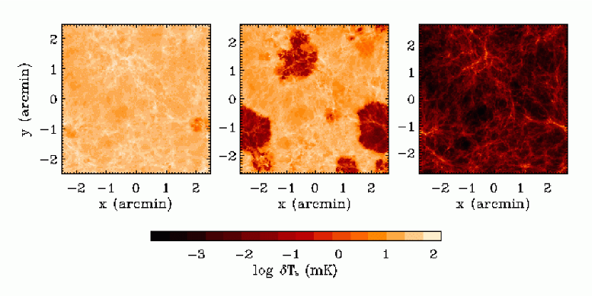
Figure 1.— The brightness temperature of the 21 cm transition at several redshifts, as predicted by the “late reionization” simulation analyzed in Furlanetto et al. (2003). Each panel corresponds to the same slice of the simulation box (with width $10h^{-1}$ comoving Mpc and depth $\Delta\nu=0.1\mbox{ MHz}$), at $z=12.1$, 9.2, and 7.6, from left to right. The three epochs shown correspond to the early, middle, and late stages of reionization in this simulation. (For details about the simulations, see Sokasian et al. 2001; Springel & Hernquist 2003a, b.)

In this paper, we present a new approach to 21 cm fluctuations. We draw an analogy between these measurements and those of the CMB: in both cases we wish to measure the level of inhomogeneity as a function of scale on the sky. Previous treatments of the 21 cm signal have focused on measuring fluctuations on a particular patch of the sky, implicitly referring to imaging observations. Here we show that a statistical treatment of the fluctuation power spectrum contains a great deal of information about reionization. Furthermore, a large set of tools for CMB predictions and data analysis has already been developed (see Hu & Dodelson 2002 for a review), so there is much to be gained by connecting the two. Indeed, some steps in this direction have already been taken by Pen (2003) and Cooray (2003), both of whom considered the effects of lensing on the 21 cm signal. The analogy with the CMB is not perfect, however, because the 21 cm signal can be separated in redshift space; in other words, we can make maps at a series of frequencies, each of which samples an independent volume. In this sense the analogy is closer to redshift surveys (e.g., Peebles 1980) or weak lensing tomography (e.g., Hu 1999). We therefore develop our formalism with explicit consideration of how multifrequency information can be used with power spectrum statistics, in effect generalizing the methodology used to analyze CMB anisotropies. After reviewing the physics of the 21 cm transition in §2, we show how to compute the angular power spectrum of 21 cm fluctuations in §3.

In §4 we show some simple applications of our approach. We give predictions for the angular power spectrum of 21 cm fluctuations from a fully neutral medium and for a simple toy model of reionization. In the former case, fluctuations in the signal are due only to large-scale structure. We show that in this regime 21 cm measurements essentially yield the power spectrum of density fluctuations (see also Pen 2003). We then show that variations in the neutral fraction during reionization distort the power spectrum.

Another advantage of our approach is that the angular power spectra are closely related to the physically observed quantities. This is especially true for the interferometers that will most likely be used to measure the redshifted 21 cm signal. Our results thus connect theoretical predictions to the potential observations. For example, inhomogeneities in the 21 cm signal must be separated from fluctuations in any foreground sources. This is particularly important because the absolute foreground signal will swamp the 21 cm signal by many orders of magnitude. While Galactic foregrounds are expected to be fairly smooth on the relevant angular scales, faint radio galaxies, starbursts, and even the galaxies responsible for reionization fluctuate strongly on arcminute scales and dominate those of the 21 cm signal by at least an order of magnitude (Di Matteo et al., 2002; Oh & Mack, 2003). These results have been used to argue that the prospects for large angular-scale measurements of the reionization epoch are dim. However, both Di Matteo et al. (2002) and Oh & Mack (2003) also pointed out that all of the (known) foreground sources have featureless power-law spectra. Both suggested that the foregrounds could therefore be removed in frequency space. As an example, consider the simple case in which every foreground source has the same spectral index. Then the foregrounds between two maps at nearby frequencies would be exactly correlated, while the 21 cm fluctuations will be uncorrelated because each frequency samples an independent volume of the IGM. Comparing two maps closely spaced in redshift therefore allows one to remove the foreground component. We show in §5 how the foreground sources can be modeled with our multi-frequency formalism. In §6 we quantify how well their contamination can be removed. We find that foregrounds are much less important than previously assumed so long as the range of allowed spectral indices for faint sources is similar to that already measured for brighter sources. Finally, we estimate in §7 how well the power spectrum can be measured with the next generation of low-frequency radio telescopes, and we conclude in §8.

When necessary, we assume a $\Lambda$CDM cosmology with $\Omega_{m}=0.3$, $\Omega_{\Lambda}=0.7$, $\Omega_{b}=0.04$, $H_{0}=100h\mbox{ km s${}^{-1}$ Mpc${}^{-1}$}$ (with $h=0.7$), and a scale-invariant primordial power spectrum with $n=1$ normalized to $\sigma_{8}=0.85$ at the present day.

2. 21 cm Radiation from the Intergalactic Medium

The optical depth of a patch of the IGM in the hyperfine transition is (Field, 1959a)

$$\tau = \frac{3c^{3}\hbar A_{10}\,n_{\rm HI}}{16k\nu_{0}^{2}\,T_{S}\,H(z)}$$ (1)

$$\approx 8.6\times 10^{-3}(1+\delta){x_{H}}\left[\frac{T_{\rm CMB}(z)}{T_{S}}\right]\left(\frac{\Omega_{b}h^{2}}{0.02}\right)$$

$$\times\left[\left(\frac{0.15}{\Omega_{m}h^{2}}\right)\,\left(\frac{1+z}{10}\right)\right]^{1/2}.$$

Here $\nu_{0}=1420.4\mbox{ MHz}$ is the rest-frame hyperfine transition frequency, $A_{10}=2.85\times 10^{-15}\mbox{ s${}^{-1}$}$ is the spontaneous emission coefficient for the transition, $T_{S}$ is the spin temperature of the IGM (i.e., the excitation temperature of the hyperfine transition), $T_{\rm CMB}=2.73(1+z)\mbox{ K}$ is the CMB temperature at redshift $z$, and $n_{\rm HI}$ is the local neutral hydrogen density. In the second equality, we have assumed sufficiently high redshifts such that $H(z)\approx H_{0}\Omega_{m}^{1/2}(1+z)^{3/2}$ (which is well-satisfied in the era we study, $z>6$). The local baryon overdensity is $1+\delta=\bar{\rho}/\rho$ and ${x_{H}}$ is the neutral fraction. The radiative transfer equation in the Rayleigh-Jeans limit then tells us that the brightness temperature of a patch of the sky (in its rest frame) is $T_{b}=T_{\rm CMB}e^{-\tau}+T_{S}(1-e^{-\tau})$. We define $\delta T(\nu)$ to be the observed brightness temperature increment between this patch, at an observed frequency $\nu$ corresponding to a redshift $1+z=\nu_{0}/\nu$, and the CMB:

$$\delta T(\nu) \approx \frac{T_{S}-T_{\rm CMB}}{1+z}\,\tau$$ (2)

$$\approx\, 23\,(1+\delta){x_{H}}\left(\frac{T_{S}-T_{\rm CMB}}{T_{S}}\right)\left(\frac{\Omega_{b}h^{2}}{0.02}\right)$$

$$\times\left[\left(\frac{0.15}{\Omega_{m}h^{2}}\right)\,\left(\frac{1+z}{10}\right)\right]^{1/2}\mbox{ mK}.$$

Assuming that the radiation background includes only the CMB, the H I spin temperature is (Field, 1958)

$$T_{S}=\frac{T_{\rm CMB}+y_{c}T_{K}+y_{{\rm Ly}\alpha}T_{{\rm Ly}\alpha}}{1+y_{c}+y_{{\rm Ly}\alpha}}.$$ (3)

The second term describes collisional excitation of the hyperfine transition, which couples $T_{S}$ to the gas kinetic temperature $T_{K}$. The coupling coefficient is

$$y_{c}=\frac{C_{10}}{A_{10}}\,\frac{T_{\star}}{T_{K}},$$ (4)

where $C_{10}(T_{K})\propto n_{H}$ is the collisional de-excitation rate of the (higher-energy) triplet hyperfine level (Allison & Dalgarno, 1969) and $T_{\star}=2\pi\hbar\nu_{0}/k=0.068\mbox{ K}$. For $T_{K}\sim 1000\mbox{ K}$, the coupling becomes strong when $1+\delta\gtrsim 5[(1+z)/20]^{2}$. The third term in equation (3) describes the Wouthuysen-Field effect, in which Ly$\alpha$ pumping couples the spin temperature to the color temperature of the radiation field $T_{{\rm Ly}\alpha}$ (Wouthuysen, 1952; Field, 1958). We note that $T_{{\rm Ly}\alpha}=T_{K}$ so long as the medium is optically thick to Ly$\alpha$ photons (Field, 1959b). Essentially, the dipole selection rules allow a transition between the two hyperfine levels of the ground state mediated by the absorption and subsequent re-emission of a Ly$\alpha$ photon. The excitation and de-excitation rates are then controlled by the color temperature of the radiation field near the line center, which (for a sufficiently large number of scatterings) must be in thermodynamic equilibrium with the gas temperature. The coupling constant for this process is

$$y_{{\rm Ly}\alpha}=\frac{P_{10}}{A_{10}}\,\frac{T_{\star}}{T_{{\rm Ly}\alpha}},$$ (5)

where $P_{10}$ is the indirect de-excitation rate of the triplet level due to absorption of a Ly$\alpha$ photon followed by decay to the singlet level. For a diffuse Ly$\alpha$ background, Madau et al. (1997) showed that

$$P_{10}\approx 1.3\times 10^{-12}J_{-21}\mbox{ s${}^{-1}$},$$ (6)

where $J_{-21}$ is the intensity of the background radiation field at the Ly$\alpha$ frequency in units of $10^{-21}\mbox{ erg cm${}^{-2}$ s${}^{-1}$ Hz${}^{-1}$ sr${}^{-1}$}$. Ly$\alpha$ pumping effectively couples $T_{S}$ and $T_{K}$ when $J_{-21}\gtrsim 1$. Ciardi & Madau (2003) argue that $J_{-21}\gg 1$ even at $z\gtrsim 20$. If so, $T_{S}\sim T_{K}$ throughout the diffuse IGM, even though the densities are well below the threshold for collisional coupling.

The spin temperature and optical depth therefore depend on the kinetic temperature of the IGM. Once Thomson scattering of CMB photons becomes inefficient at the thermal decoupling redshift $z_{d}\sim 140$, the IGM cools adiabatically until the first objects collapse (Couchman & Rees, 1986). During this era, $T_{K}<T_{\rm CMB}$. The cooling trend reverses itself as soon as significant structure begins to form, but the subsequent temperature evolution is both inhomogeneous and highly uncertain. While early estimates suggested that Ly$\alpha$ photons themselves would inject significant thermal energy into the IGM, Chen & Miralda-Escudé (2003) showed that this heating channel is in reality quite slow. Instead, X-rays (primarily from supernovae or accreting black holes) and shocks are likely to control the temperature evolution of the IGM. We expect shocks to heat overdense structures like sheets, filaments, and virialized halos to $T_{K}>T_{\rm CMB}$ and radiative feedback from stars and quasars to heat the rest of the gas. Most estimates suggest that the two processes will rapidly heat the IGM to $T_{K}>T_{\rm CMB}$ (Venkatesan et al., 2001; Chen & Miralda-Escudé, 2003; Gnedin & Shaver, 2003). The topology of the two cases of course differs; shock heating will tend to exaggerate brightness temperature differences by separating warm, dense regions from cool voids, while X-ray heating will induce a smooth temperature distribution.

In developing our formalism, we allow $\delta T(\nu)$ to depend on the parameters $\delta,{x_{H}},$ and $T_{S}$. This is the most general case possible (once the cosmological parameters are fixed) and allows one to incorporate the full range of physics when necessary. However, the arguments above suggest that the situation most relevant to observations has $T_{S}\sim T_{K}\gg T_{\rm CMB}$. In this limit, the temperature factor in equation (2) approaches unity and the signal is independent of $T_{S}$. Thus we essentially assume an era of significant X-ray heating; in this scenario, the extra heating in shocked dense regions can be ignored. For simplicity, we will restrict ourselves to this case for the illustrative examples in §4. We emphasize that this is, however, an important assumption. If, for example, significant heating does not occur until the early stages of reionization, $\delta T_{b}$ will have a much more complicated distribution than we consider here.

Finally, to orient the reader, we note that an observed bandwidth $\Delta\nu$ corresponds to a comoving distance

$$L\approx 1.7\left(\frac{\Delta\nu}{0.1\mbox{ MHz}}\right)\left(\frac{1+z}{10}\right)^{1/2}\left(\frac{\Omega_{m}h^{2}}{0.15}\right)^{-1/2}\mbox{ Mpc},$$ (7)

while a given angular scale $\Delta\theta$ corresponds to

$$R\approx 1.9\left(\frac{\Delta\theta}{1^{\prime}}\right)\left(\frac{1+z}{10}\right)^{0.2}h^{-1}\mbox{ Mpc}$$ (8)

over the relevant redshift range.

3. Basic Formalism

We now show how to compute the angular power spectrum of 21 cm fluctuations. Unfortunately, a given patch of the sky observed with frequency bandwidth $\Delta\nu$ does not correspond directly to a physical volume of the Universe because the observation is performed in redshift space: peculiar velocities can move a parcel of gas into or out of this channel. However, redshift space distortions will be unimportant if $\Delta\nu/\nu>v/c$ where $v$ is the typical random bulk velocity of the gas. The importance of redshift space distortions is determined by the ratio

$${\cal R}={\Delta\nu/\nu\over v/c}\approx 20\times\left[{(1+z)\over 11}\right]\times\left[{\Delta\nu\over 0.2\ {\rm MHz}}\right]\times\left[{v/c\over 10^{-4}}\right]^{-1}$$ (9)

For large values of ${\cal R}$, redshift distortions have only a marginal effect. Furlanetto et al. (2003) have shown that, for typical survey geometries, redshift space distortions amplify the signal by at most $\sim 25\%$ (see also Tozzi et al. 2000). For simplicity we will ignore them in what follows. In future work, we will examine the significance of redshift distortions in detail using numerical simulations and asses what cosmological information can be extracted from their detection.

If redshift distortions can be neglected, there is a one-to-one correspondence between frequency and redshift. The bandwidth of the experiment is characterized by some response function $W(\nu)$. The observed brightness temperature is of the form

$$T({\hat{\bf n}},\nu)=T_{0}(r_{0})\int drW_{r_{0}}(r)\psi({\hat{\bf n}},r),$$ (10)

where ${\hat{\bf n}}$ is the direction of observation, $T_{0}$ is a normalization constant which depends on redshift and $\psi({\hat{\bf n}},r)$ is the dimensionless brightness temperature, $\psi({\hat{\bf n}},r)=(1+\delta)x_{H}(T_{S}-T_{\rm CMB})/T_{S}$. Note that $\delta T(\nu)=T_{0}(r_{0})\psi({\hat{\bf n}},r)$ in equation (2). The projection window $W_{r0}(r)$ is a function peaked at $r_{0}$, the radial distance corresponding to the observed frequency $\nu$, and has a width $\delta r$.

We can expand $\psi({\bf x})$ as a Fourier series,

$$\psi({\bf x}) = \int{d^{3}k\over(2\pi)^{3}}\ {\hat{\psi}}({\bf k})e^{i{\bf k}\cdot{\bf x}}$$ (11)

$$= \int{d^{3}k\over(2\pi)^{3}}\ {\hat{\psi}}({\bf k})\sum_{lm}4\pi i^{l}j_{l}(kr)Y_{lm}^{*}(\hat{\bf k})Y_{lm}({\hat{\bf n}}),$$

where $j_{l}(x)$ are the spherical Bessel functions and $Y_{lm}({\hat{\bf n}})$ are the spherial harmonics. The statistics of $\psi$ are determined by its power spectrum,

$$\langle{\hat{\psi}}({\bf k}_{1}){\hat{\psi}}({\bf k}_{2})\rangle=(2\pi)^{3}{\delta^{D}}({\bf k}_{1}+{\bf k}_{2}){P_{\psi}}(k_{1}).$$ (12)

We use equations (10) and (11) to calculate the spherical harmonic decomposition $a_{lm}$ of the observed temperature:

$$a_{lm}(\nu) = 4\pi i^{l}\int{d^{3}k\over(2\pi)^{3}}\ {\hat{\psi}}({\bf k})\alpha_{l}(k,\nu)Y_{lm}^{*}(\hat{\bf k}),$$

$$\alpha_{l}(k,\nu) = T_{0}(r_{0})\int drW_{r_{0}}(r)j_{l}(kr).$$ (13)

We can define the angular power spectrum as

$$\langle a_{l_{1}m_{1}}(\nu_{1})a^{*}_{l_{2}m_{2}}(\nu_{2})\rangle = \delta_{l_{1}l_{2}}\delta_{m_{1}m_{2}}C_{l_{1}}(\nu_{1},\nu_{2})$$

$$C_{l}(\nu_{1},\nu_{2}) = 4\pi\int{d^{3}k\over(2\pi)^{3}}{P_{\psi}}(k)\alpha_{l}(k,\nu_{1})\alpha_{l}(k,\nu_{2})$$ (14)

$$= 4\pi\int{dk\over k}\Delta^{2}_{\psi}(k)\alpha_{l}(k,\nu_{1})\alpha_{l}(k,\nu_{2}).$$

Here $\Delta^{2}_{\psi}(k)=k^{3}P_{\psi}/(2\pi^{2})$ and we have used the isotropy of $P_{\psi}$. This formula encodes both the case of the power spectrum of maps at one particular frequency (when $\nu_{1}=\nu_{2}$) as well as the correlations between maps at different frequencies. Equation (3) forms the basis for the analysis that makes it possible to relate the 21 cm fluctuations to the evolution of the ionization state of the IGM. Note that the $C_{l}$’s approach zero as $\nu_{1}$ and $\nu_{2}$ depart from each other for two reasons: because the frequency-space window functions no longer overlap in this limit and because the fluctuations in the IGM are uncorrelated on large scales. The latter property can be used to separate the 21 cm signal from contamination by foreground sources that vary smoothly with frequency.

We can investigate the behavior of equation (3) by considering various limits. We want to understand how equation (3) depends on the width of the response function, $\delta r$ (which describes the bandwidth of the observation). The figure of merit is $l\delta r/r$ (i.e. the ratio of the radial to transverse scales probed by the observation). We first consider the limit in which the response function can be considered to be a delta function, $l\delta r/r\ll 1$. In that case,

$$\alpha_{l}\approx T_{0}(r_{0})j_{l}(kr_{0}),$$ (15)

so that

$$C_{l}(\nu,\nu) \approx 4\pi T_{0}^{2}(r_{0})\int{dk\over k}\Delta^{2}_{\psi}(k)j_{l}^{2}(kr_{0}).$$ (16)

In the limit in which the power spectrum can be approximated by a power law, $\Delta^{2}_{\psi}(k)=(k/k_{*})^{n}$ we then have

$$C_{l}(\nu,\nu) \approx 4\pi T_{0}^{2}(r_{0})\Delta^{2}_{\psi}(l/r_{0})\int{dx\over x}(x/l)^{n}j_{l}^{2}(x)$$

$${l(l+1)C_{l}(\nu,\nu)\over 2\pi} \approx T_{0}^{2}(r_{0})\Delta^{2}_{\psi}(l/r_{0})f(n)$$

$$f(n,l) = {\sqrt{\pi}(l+1)\Gamma[1-n/2]\Gamma[l+n/2]\over 2l^{n-1}\Gamma[(3-n)/2]\Gamma[2+l-n/2]}.$$ (17)

With this definition $f(n,l)$ is a very weak function of both $l$ and $n$ and it is normalized so that $f(0,l)=1$. Thus in this limit $(l\delta r/r\ll 1)$, the temperature fluctuations simply trace the underlying $\psi$ fluctuations,

$${l(l+1)C_{l}(\nu,\nu)\over 2\pi}\propto T_{0}^{2}(r_{0})\Delta^{2}_{\psi}(l/r_{0}).$$ (18)

We now consider the opposite regime, $l\delta r/r\gg 1$, the large bandwidth or Limber limit (Limber, 1953; Peebles, 1980). We can approximate the integral in a different way,

$$C_{l}(\nu,\nu) = 4\pi\int{d^{3}k\over(2\pi)^{3}}{P_{\psi}}(k)\alpha_{l}^{2}(k,\nu)$$ (19)

$$= 4\pi T_{0}^{2}\int dr_{1}W(r_{1})\int dr_{2}W(r_{2})$$

$$\times\int{4\pi k^{2}dk\over(2\pi)^{3}}{P_{\psi}}(k)j_{l}(kr_{1})j_{l}(kr_{2}).$$

The Bessel functions $j_{l}(x)$ are very small for $x<l$ and start to oscillate when $x\sim l$. Thus, the integral over $k$ will receive contributions only from a region around $k\sim l/r$ with width of order $\Delta k\sim 1/\delta r$. Modes with $k>k+\Delta k$ will be out of phase for typical separations of the two points $r_{1}$ and $r_{2}$. In this regime we can approximate ${P_{\psi}}(k)\approx{P_{\psi}}(l/r_{1})$. The integral over $k$ is then proportional to ${\delta^{D}}(r_{1}-r_{2})/r_{1}^{2}$ so that

$$C_{l}(\nu_{1},\nu_{2}) = T_{0}^{2}\int drW^{2}(r){P(l/r)\over r^{2}}$$

$${l(l+1)C_{l}(\nu,\nu)\over 2\pi} \propto T_{0}^{2}\Delta^{2}_{\psi}(l/r_{0}){r_{0}\over l\delta r}.$$ (20)

This is the standard Limber’s equation, widely used in the context of weak lensing (e.g. Kaiser 1992).

Equations (18) and (3) are easy to understand. For a sufficiently narrow frequency response ($l\delta r/r\ll 1$), the angular fluctuations directly trace those of the underlying $\psi$ field. However, for a surface of finite width $\delta r$ only those modes with radial $k\lesssim 1/\delta r$ can contribute because the response function averages out larger $k$ modes. Thus when the surface becomes too thick in the radial direction, angular fluctuations are no longer of order $\sim k^{3}P(k)$ but become $\sim k^{2}P(k)/\delta r$, as seen in equation (3).

To estimate the $l$ at which the width of the surface begins to damp the fluctuations, we can consider an Einstein de-Sitter universe in which $a(\tau)=(\tau/\tau_{0})^{2}$, where $a$ is the scale factor and $\tau$ is the conformal time. In this case $\delta\tau/\tau=(1/2)\delta a/a=(1/2)\Delta\nu/\nu$. Thus, the changes in radial distance $r=\tau_{0}-\tau$ are just

$$|{\delta r\over r}|\approx{1\over 2\sqrt{1+z}}\ {\Delta\nu\over\nu},$$ (21)

where $\nu$ is the observed frequency, $\nu=\nu_{0}/(1+z)$. For $\Delta\nu=0.2\ {\rm MHz}$ the corresponding value of $l$ from equation (21) is $l\sim 5000$, or arcminute scales. The damping of fluctuations for large bandwidths has important implications for the choice of $(\Delta\nu,l)$ in a given observation (see Figure 4 below and the discussion thereof).

4. Simple Model for the Correlations of the Brightness Temperature

In this section we will make a simple model for the correlations of the dimensionless brightness temperature, $\psi$. A more detailed study using simulations is left for future work.

We assume that $T_{S}\gg T_{\rm CMB}$ so that $\psi=x_{H}(1+\delta)$. To calculate the power spectrum of $\psi$ we need a model for the correlations of the neutral fraction, $x_{H}$. We will follow a similar treatment as that used to model the effect of patchy reionization on CMB anisotropies (e.g. Gruzinov & Hu 1998; Knox et al. 1998). For simplicity, we will model the the fluctuations in $x_{H}$ as if they were produced by a set of uncorrelated “bubbles” of typical size $R$. We denote the average value of ${x_{H}}$ as ${{\bar{x}}_{H}}$. We allow both $R$ and ${{\bar{x}}_{H}}$ to depend on redshift. Under this simplifying assumption we can model the correlations as

$$\langle x_{H}({\bf x}_{1})x_{H}({\bf x}_{2})\rangle={{\bar{x}}_{H}}^{2}+({{\bar{x}}_{H}}-{{\bar{x}}_{H}}^{2})f(x_{12}/R),$$ (22)

where $f(x)$ is a function with the following limits: $f(x)\approx 1$ for $x\ll 1$ and $f(x)\approx 0$ for $x\gg 1$. The details of this function depend on the shape of the bubbles. If the bubbles are correlated, one should interpret $R$ as an effective size that depends on the correlation length between distinct bubbles. To calculate observables, we will take $f(x)=\exp(-x^{2}/2)$.

The correlations of $\psi$, $\mu(x_{12})\equiv\langle\psi({\bf x}_{1})\psi({\bf x}_{2})\rangle-\langle\psi\rangle^{2}$, become

$$\mu(x_{12}) = [{{\bar{x}}_{H}}^{2}+({{\bar{x}}_{H}}-{{\bar{x}}_{H}}^{2})f(x_{12}/R)]\xi(x_{12})+$$ (23)

$$({{\bar{x}}_{H}}-{{\bar{x}}_{H}}^{2})f(x_{12}/R)+\eta(x_{12})[2{{\bar{x}}_{H}}+\eta(x_{12})],$$

where $\xi(x_{12})=\langle\delta({\bf x}_{1})\delta({\bf x}_{2})\rangle$ is the correlation function of the density field and $\eta(x_{12})=\langle\delta({\bf x}_{1})x_{H}({\bf x}_{2})\rangle$ gives the cross correlation between the density and neutral fraction fields. To keep things as simple as possible we will ignore this last term in what follows. We will explore the consequences of including it in future work. The correlation function is related to the density power spectrum by

$$\xi(r)=\int{dk\over k}{\Delta^{2}}_{\rho}(k){\sin kr\over kr}.$$ (24)

Equation (23) has the following limits:

$$\mu(x_{12}) \approx {{\bar{x}}_{H}}\xi(x_{12})+({{\bar{x}}_{H}}-{{\bar{x}}_{H}}^{2})\ \ (x_{12}\ll R),$$

$$\mu(x_{12}) \approx {{\bar{x}}_{H}}^{2}\xi(x_{12})\ \ \ \ \ \ \ \ \ \ \ \ \ \ \ \ \ \ \ (x_{12}\gg R).$$ (25)

When $x_{12}\gg R$ both points are basically independent as far as the correlations in $x_{H}$ are concerned, so the correlations are given by those of the density field times the probability that each of the two points falls in a neutral region, ${{\bar{x}}_{H}}^{2}$. On scales smaller than the “bubble” size, both points fall either inside or outside a “bubble” so only one factor of ${{\bar{x}}_{H}}$ multiplies $\xi$. On top of the fluctuations produced by the density there are those created by the presence of the bubbles, $({{\bar{x}}_{H}}-{{\bar{x}}_{H}}^{2})$. To illustrate the behavior of equation (23) we can take the correlation function of the density to be a power law, $\xi(x)=(x/x_{0})^{-n}$. Moreover, assume that $x_{0}<R$ and ${{\bar{x}}_{H}}\sim 0.5$. On scales smaller than $x_{0}$, $\mu(x)\approx{{\bar{x}}_{H}}(x/x_{0})^{-n}$. In the range $x_{0}<x<R$, $\mu(x)\approx{{\bar{x}}_{H}}(1-{{\bar{x}}_{H}})$, while for $x\gg R$, $\mu(x)\approx{{\bar{x}}_{H}}^{2}(x/x_{0})^{-n}$. Thus there is a feature in the correlation function on the scale of the bubbles. In this simple model the $\psi$ correlations trace the matter correlations on both large and small scales (but with different amplitudes). On scales intermediate between the size of the bubbles and the non-linear scale the correlation function flattens out.

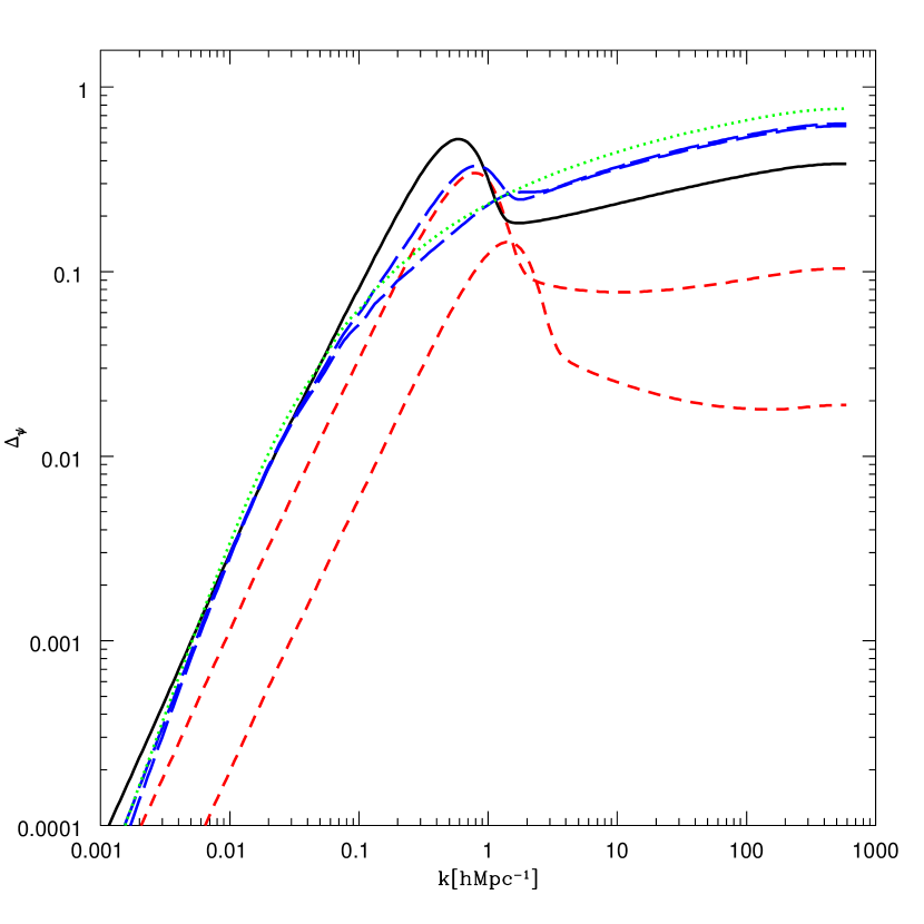
Figure 2.— Power spectrum of $\psi$ fluctuations, $\Delta_{\psi}^{2}=k^{3}P_{\psi}/2\pi^{2}$, in the model described in the text. The lines correspond to $z=12,11,10,9$, and $8$. At $z=10$ (solid black line), ${{\bar{x}}_{H}}=1/2$. The long-dashed blue lines correspond to $z=12$ and $11$ at the beginning of reionization and the short-dashed red lines to $z=9$ and $8$. The dotted green line shows the power spectrum of the density field at $z=10$. Note that we use the linear dark matter power spectrum in computing the density fluctuations.

We can Fourier transform equation (23) (with $\eta=0$) to obtain an expression for the power spectrum of $\psi$,

$${\Delta^{2}}_{\psi}(k) = {{\bar{x}}_{H}}^{2}{\Delta^{2}}_{\rho}(k)+({{\bar{x}}_{H}}-{{\bar{x}}_{H}}^{2}){\Delta^{2}}_{x\rho}(k)$$ (26)

$$+({{\bar{x}}_{H}}-{{\bar{x}}_{H}}^{2}){\Delta^{2}}_{x}(k),$$

where we have introduced

$${\Delta^{2}}_{x}(k) = {k^{3}{\hat{f}}(k)\over 2\pi^{2}},$$

$${\Delta^{2}}_{x\rho}(k) = {k^{3}\over 2\pi^{2}}\int{d{\bf k}^{\prime}\over(2\pi)^{3}}P_{\rho}({\bf k}-{\bf k}^{\prime}){\hat{f}}({\bf k}^{\prime}),$$ (27)

with ${\hat{f}}(k)$ the Fourier transform of $f(x)$ and $P_{\rho}({\bf k})$ is the power spectrum of the density fluctuations.

In Figure 2 we show the power spectrum of $\psi$ calculated from equation (26). For illustrative purposes, we used a simple model for the mean neutral fraction as a function of redshift,

$${{\bar{x}}_{H}}(z)={1\over 1+\exp[-(z-z_{o})/\Delta z]},$$ (28)

with $z_{0}=10$ and $\Delta z=0.5$. For the correlation length $R$ we used a maximum value of $3h^{-1}{\rm Mpc}$ when ${{\bar{x}}_{H}}=0.5$ and smaller values when ${{\bar{x}}_{H}}$ deviates in both directions from $0.5$ so as to keep the number density of bubbles fixed. We show results for, $(z,{{\bar{x}}_{H}},R)=$ (12,0.98,1.24), (11,0.88,2.24), (10,0.5,3), (9,0.12,2.24), (8,0.02,1.24). For comparison, we also show the power spectrum of matter fluctuations at redshift $z=10$. The form of this choice for the evolution of the mean neutral fraction is motivated by numerical simulations of reionization (e.g. Figures 5 and 9 of Sokasian et al. 2003a, b, respectively). Note that we have simply used the linear dark matter power spectrum at the appropriate redshift in computing $\Delta^{2}_{\rho}$ for the Figure. In reality, of course, we should use the full gas power spectrum, which includes the nonlinear growth of structure on small scale and smoothing due to the finite pressure of the gas. The differences are, however, not large (see, for example, Figure 2 of Furlanetto et al. 2003), so the linear dark matter spectrum will suffice for our purposes here. We will consider modifications due to the true power spectrum in future work.

Before reionization begins, the power spectrum of $\psi$ is simply the power spectrum of the matter fluctuations. As the neutral fraction decreases it develops a feature on the scale of the bubbles, roughly at $k\sim 2/R$. The feature has maximum amplitude when ${{\bar{x}}_{H}}=0.5$. As the neutral fraction decreases further, the 21 cm fluctuations disappear because there is no longer any more neutral hydrogen to emit radiation. Note that when the bubbles appear, the power spectrum on the largest scales is a power law $\Delta^{2}_{\psi}\propto k^{3}$, corresponding to Poisson fluctuations. That is, the Poisson fluctuations induced by the discrete nature of the bubbles dominates over the fluctuations resulting from $\delta$.

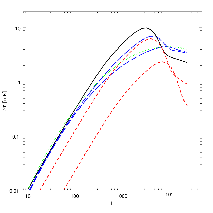
Figure 3.— Angular power spectrum of 21cm fluctuations at $z=12,11,10,9$, and $8$ in the model described in the text (the curves are the same as in Figure 2). The bandwidth is $0.2\mbox{ MHz}$.

In Figure 3 we show the corresponding angular power spectrum $\delta T=[l(l+1)C_{l}/2\pi]^{1/2}$ with a window function $W_{r_{0}}(r)$ of Gaussian shape, centered at the appropriate redshift and with a full width at half maximum of $0.2$ MHz. The angular power spectrum traces the behavior of the 3D power spectrum shown in Figure 2. It develops a feature on the scale of the bubbles, $l\sim kr\sim 2r/R$. We emphasize that the precise shapes of the curves like those in Figures 2 and 3 depend on the morphology of the ionized regions. Here, we have adopted a simple model in which these “bubbles” are described by spheres whose size evolves simply with redshift. In reality, the ionized regions have complicated morphology and evolution, as indicated by Figure 1, that will likely imprint more complex features into the power spectra than suggested by Figures 2 and 3. We will examine these issues further in due course.

On small scales, the angular power spectrum in Figure 3 changes slope and stops tracing $\Delta_{\psi}$. This occurs when the window in frequency becomes too wide and we enter into the Limber regime [equation (3)], where the angular fluctuations are damped by one power of $k$. To illustrate this further, we plot the angular power spectrum for several spectral widths in Figure 4. As the width of the filter increases, the level of fluctuations decreases. The Figure shows that the damping is insignificant until the Limber regime is reached at $l\delta r/r\sim 1$; in the regime where the fluctuations are dominated by the bubbles, this happens when $\delta r/R\sim 1$. For bandwidths larger than this, the level of fluctuations scales as $1/\delta r\propto 1/\Delta\nu$ for a fixed angular scale. On the other hand, the signal per channel is proportional to the bandwidth. Thus, if one is interested in a particular angular scale $l$, it is best to choose the bandwidth $\Delta\nu$ such that $l\delta r/r\lesssim 1$.

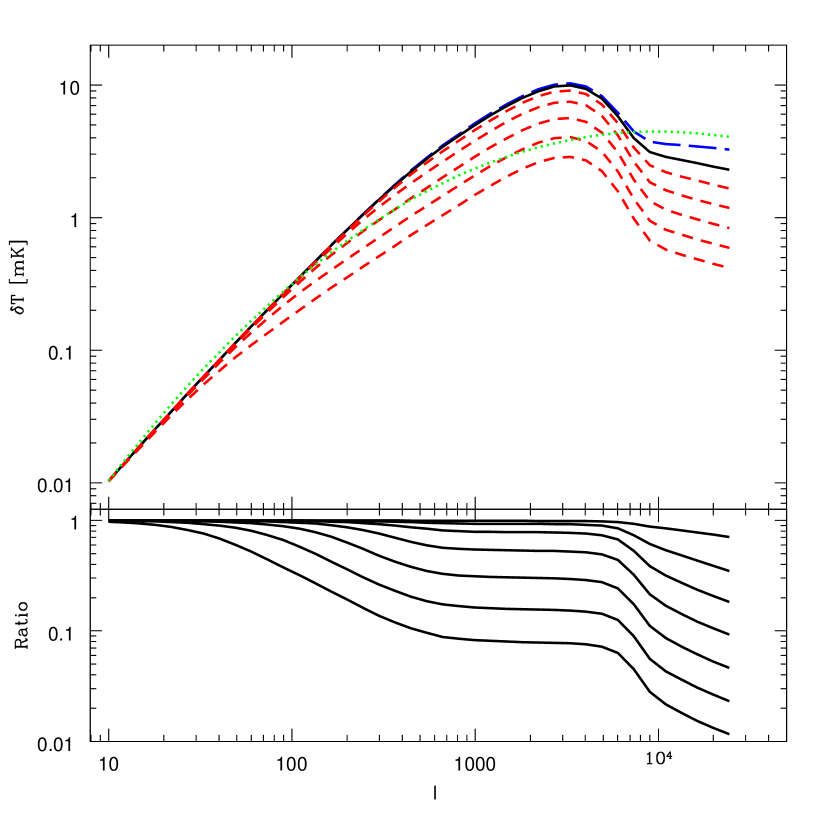
Figure 4.— Top panel: Angular power spectrum at redshift $z=10$ for observations done with filters of full width at half maximum (0.1, 0.2, 0.4, 0.8, 1.6, 3.2, 6.4) MHz. The dotted line in the top panel shows the power spectrum of $\delta$ at $z=10$. Bottom panel: Ratio between the power spectra in the top panel and one corresponding to a delta function filter.

5. Modeling the Contaminants

One of the major challenges in observing this signal is separating it from the many other (stronger) low-frequency radio sources. There are several potential sources of noise, but those associated with foreground sources are likely to be smooth in frequency space. In this section we will show how this smoothness can be used to remove this contamination. We will explicitly consider point source foregrounds, as discussed by Di Matteo et al. (2002) and Oh & Mack (2003), but our method can be easily be extended to other types (such as diffuse Galactic synchrotron emission), provided that their power spectra can be estimated.

Let us assume that there is a collection of different types of sources with a range of spectral indices $\zeta$. We describe them by a luminosity function $d^{2}n/dSd\zeta$, which gives the average number of sources per steradian per unit flux $S$ and spectral index $\zeta$. We will assume that the sources are clustered but not necessarily that sources of different spectral indices are perfectly correlated. The clustering on the sky is described by the angular power spectrum,

$$\langle a^{c}_{l_{1}m_{1}}(\zeta_{1})a^{c}_{l_{2}m_{2}}(\zeta_{2})\rangle = \delta_{l_{1}l_{2}}\delta_{m_{1}m_{2}}C_{l_{1}}^{c}(\zeta_{1},\zeta_{2})$$

$$= \delta_{l_{1}l_{2}}\delta_{m_{1}m_{2}}{\cal C}^{c}_{l_{1}}(\zeta_{1},\zeta_{2})\sqrt{C_{l_{1}}^{c}(\zeta_{1})C_{l_{1}}^{c}(\zeta_{2})},$$

where $C_{l}^{c}(\zeta_{1},\zeta_{2})$ is the cross correlation between the populations and $C_{l}^{c}(\zeta)=C_{l}^{c}(\zeta,\zeta)$ is the auto correlation of a given population. These are nothing more than the Legendre transforms of the respective correlation functions. We have also introduced the correlation coefficient ${\cal C}^{c}_{l}(\zeta_{1},\zeta_{2})=C_{l}^{c}(\zeta_{1},\zeta_{2})/\sqrt{C_{l}^{c}(\zeta_{1})C_{l}^{c}(\zeta_{2})}$.

The power spectrum of fluctuations on the sky produced by these sources is given by,

$$C_{l}(\nu_{1},\nu_{2}) = \int dSd\zeta{d^{2}n\over dSd\zeta}S^{2}\left({\nu_{1}\over\bar{\nu}}\right)^{\zeta}\left({\nu_{2}\over\bar{\nu}}\right)^{\zeta}$$

$$+ C_{l}^{c}(\bar{\zeta})\int dS_{1}d\zeta_{1}{d^{2}n\over dS_{1}d\zeta_{1}}\int\ dS_{2}d\zeta_{2}{d^{2}n\over dS_{2}d\zeta_{2}}$$

$$\times {\cal C}^{c}_{l}(\zeta_{1},\zeta_{2})\sqrt{C_{l_{1}}^{c}(\zeta_{1})\over C_{l}^{c}(\bar{\zeta})}\sqrt{C_{l}^{c}(\zeta_{2})\over C_{l}^{c}(\bar{\zeta})}\left({\nu_{1}\over\bar{\nu}}\right)^{\zeta_{1}}\left({\nu_{2}\over\bar{\nu}}\right)^{\zeta_{2}}.$$

The first term is the Poisson contribution and the second comes from the clustering of the sources. We have denoted the average spectral index by $\bar{\zeta}$.

We will eventually show that what interferes with a measurement of the 21 cm signal is the fact that the foreground maps in different frequencies may not be perfectly correlated. If the maps were perfectly correlated, then one could in some sense subtract the map at one frequency from another and clean the map of all contamination. In our simple model the presence of sources with several spectral indices is at the heart of the fact that maps at different frequencies become uncorrelated.

To make some progress, we adopt some assumptions about the different quantities that enter into equation (5). We will take

$${d^{2}n\over dSd\zeta}={dn\over dS}f(\zeta)={dn\over dS}\ \ {e^{-(\zeta-\bar{\zeta})^{2}/2\delta\zeta^{2}}\over\sqrt{2\pi}\delta\zeta},$$ (31)

where $\delta\zeta$ measures the range of spectral indices of the sources. This Gaussian form is a reasonable description of the spectral index distribution of low-frequency radio sources measured by Cohen et al. (2003). We need to model the correlation coefficient between different sources. We know that ${\cal C}_{l}(\zeta,\zeta)=1$ and should decay as the two $\zeta$’s depart from each other. We will take

$${\cal C}(\zeta_{1},\zeta_{2})=e^{-(\zeta_{1}-\zeta_{2})^{2}/2\sigma_{\zeta}^{2}},$$ (32)

where $\sigma_{\zeta}$ measures how sources with different spectral indices become uncorrelated. For simplicity, we will assume that ${\cal C}$ is independent of $l$. This could be relaxed easily but would make our expression a bit more complicated. To the extent that all sources are tracing the same underlying distribution of matter, they should be perfectly correlated, even if their bias is somewhat different. Only the stochastic part of the bias contributes to the loss of correlation. Thus we expect $\sigma_{\zeta}$ to be large compared to $\delta\zeta$; that is, all the sources should be well correlated on the sky. Finally, we will approximate

$$\sqrt{C_{l}^{s}(\zeta)\over C_{l}^{s}(\bar{\zeta})}\approx 1+{1\over 2}{d\ln C_{l}\over d\ln\zeta}({\zeta\over\bar{\zeta}}-1),$$ (33)

meaning that we will compute quantities of interest only to lowest order in the change of clustering with population.

We use the above formulae to calculate the correlation coefficient between maps at different frequencies,

$$I_{l}(\nu_{1},\nu_{2})={C_{l}(\nu_{1},\nu_{2})\over\sqrt{C_{l}(\nu_{1},\nu_{1})C_{l}(\nu_{2},\nu_{2})}}.$$ (34)

We calculate $I_{l}(\nu_{1},\nu_{2})$ as a series in $\ln(\nu_{1}/\nu_{2})$ and to lowest order in ${d\ln C_{l}/d\ln\zeta}$ and $\delta\zeta/\sigma_{\zeta}$ and obtain

$$I_{l}(\nu_{1},\nu_{2}) \approx 1-{1\over 2}\delta\zeta^{2}\ln^{2}(\nu_{1}/\nu_{2})\Biggl{\{}{{\gamma}\over 1+{\gamma}}+{(1+2{\gamma})\over(1+{\gamma})^{2}}\left({\delta\zeta\over\sigma_{\zeta}}\right)^{2}$$ (35)

$$+ \left({d\ln C_{l}\over d\ln\zeta}\delta\zeta\right)^{2}$$

$$\times\left[{{\gamma}\over 4(1+{\gamma})^{2}}-{1+2{\gamma}(1+{\gamma})\over 2(1+{\gamma})^{3}}\left({\delta\zeta\over\sigma_{\zeta}}\right)^{2}\right]\Biggr{\}},$$

where ${\gamma}$ measures the importance of the Poisson term relative to the term due to clustering:

$${\gamma} = {C_{l}^{poisson}\over C_{l}^{cluster}},$$

$$C_{l}^{poisson} = \int dS{dn\over dS}S^{2},$$

$$C_{l}^{cluster} = C_{l}^{s}(\bar{\zeta}){\cal I}^{2},$$

$${\cal I} = \int dS{dn\over dS}S.$$

These are the standard formulae for the Poisson and clustering contributions for a single population of sources (e.g. Peebles 1980). Equivalently from equation (5) and to lowest order in $\delta\zeta/\sigma_{\zeta}$ and $d\ln C_{l}/d\ln\zeta$ we find

$$C_{l}(\bar{\nu},\bar{\nu})=C_{l}^{poisson}+C_{l}^{s}(\bar{\zeta}){\cal I}^{2}.$$ (37)

We can point out a few interesting things about equation (35). First of all, the departure from unity is proportional to $\delta\zeta^{2}\ln^{2}(\nu_{1}/\nu_{2})$. As expected, there is a loss of correlation only to the extent that there are sources with a variety of spectral indices in the mix. There are several contributions to the loss of correlation. The first term on each line (proportional to ${\gamma}/[1+{\gamma}]$) is a direct consequence of the Poisson part; they go to zero as ${\gamma}\rightarrow 0$. They occur because, if the Poisson contribution is dominant, there is a chance of getting a different spectral index in different regions of the sky. That is to say, there are a few sources in any given mode on the sky and so the fluctuations in the spectral index of actual sources that happen to be in each region will lead to patterns on the sky that are not identical at different frequencies. The other terms come from the clustering part (they go to zero as ${\gamma}\rightarrow\infty$). Those terms only appear if different sources are not perfectly correlated (terms proportional to $\delta\zeta/\sigma_{\zeta}$) or if they cluster differently (terms proportional to ${d\ln C_{l}/d\ln\zeta}$).

The main point of equation (35) is that the difference between the cross-correlation and unity scales as $\delta\zeta^{2}\ln^{2}(\nu_{1}/\nu_{2})$, so it should be quite small. This will imply that the noise from the smooth foregrounds is unimportant.

6. The Effect of Contamination

In this section we will show how the frequency information can be used to discriminate the 21 cm signal from sources of contamination. The basic point is that while the contaminants are presumed to be smooth as a function of frequency, the 21 cm signal varies very rapidly. A small change in frequency of order a fraction of a MHz is already enough to sample an effectively different part of the Universe. In what follows, we will present two derivations that show that the measurement is only contaminated by the parts of the foregrounds that are uncorrelated between neighboring frequencies. For simplicity we will only consider two frequencies and show how the combination of information from both can significantly reduce the level of contamination. Clearly to make full use of the data set one should consider all the frequencies. Here we illustrate the method with just two but the generalization is trivial.

6.1. Fisher matrix

To illustrate how the cleaning works let us take a simple model for the data,

$$a_{lm}(\nu)=a^{21cm}_{lm}(\nu)+a^{f}_{lm}(\nu)+a^{noise}_{lm}(\nu).$$ (38)

The three terms are the 21 cm signal, foreground contamination, and detector noise. We will assume that we make $N_{l}$ measurements at two separate frequencies, $\nu_{1}$ and $\nu_{2}$, so that the data vector is of the form ${\bf x}_{i}=(a_{lm}(\nu_{1}),a_{lm}(\nu_{2}))$ with $i=1,\cdots N_{l}$. We will assume that both the 21 cm signal and the detector noise are uncorrelated between the two frequencies while the foregrounds have a correlation coefficient $I$, very close to unity. In that case the correlation matrix of the data is

$$\langle{\bf x}_{i}{\bf x}_{j}^{\dagger}\rangle ={\bf C}_{ij}= \delta_{ij}\left[C^{f}_{l}\left(\begin{array}[]{cc}1&I\sqrt{\beta}\\ \sqrt{\beta}I&\beta\\ \end{array}\right)\right.$$ (41)

$$\left.+C_{l}^{21cm}\left(\begin{array}[]{cc}1&0\\ 0&1\\ \end{array}\right)+C_{l}^{N}\left(\begin{array}[]{cc}1&0\\ 0&1\\ \end{array}\right)\right],$$ (46)

where $\beta$ characterizes the frequency dependence of the foregrounds and $C_{l}^{N}$ gives the power spectrum of the noise, which for simplicity we assumed equal in both channels and uncorrelated between the different $N_{l}$ measurements (see §7).

We will assume that the fluctuations are Gaussian and that we wish to estimate the three parameters of the model, ${\bf p}=(C^{f}_{l},\beta,C_{l}^{21cm})$, simultaneously. We can calculate the expected error bars from the Fisher matrix ${\cal F}$,

$${\cal F}_{i_{1},i_{2}}={1\over 2}{\rm Tr}\left[{\bf C}^{-1}{\partial{\bf C}\over\partial{\bf p}_{i_{1}}}{\bf C}^{-1}{\partial{\bf C}\over\partial{\bf p}_{i_{2}}}\right]$$ (47)

where $i_{1}$, $i_{2}$ run over the three parameters. The inverse of the Fisher matrix gives the expected covariance matrix of the recovered parameters (see Tegmark, Taylor & Heavens 1997 for a summary of the Fisher matrix technique). In particular, the error in the recovered 21 cm power spectrum is simply

$$(\Delta C_{l}^{21cm})^{2} ={\cal F}^{-1}_{3,3}$$

$$={2\over N_{l}} \left[\left(C_{l}^{21cm}+C_{l}^{N}+{2\beta\over(1+\beta)}(1-I)C_{l}^{f}\right)^{2}\right.$$

$$\left.+\left({2\beta(1-I)C_{l}^{f}\over(1+\beta)}\right)^{2}\right],$$ (48)

where we have assumed $C_{l}^{f}\gg C_{l}^{21cm},C_{l}^{N}$.

We see that the foreground power spectrum is suppressed by a factor $1-I$; so, as long as $(1-I)C_{l}^{f}<C_{l}^{21cm}$ the noise introduced by foregrounds can handled with this technique.

6.2. Another derivation

We can obtain the same result as above by considering the following problem. Assume we measure the $a_{lm}$’s at two different frequencies and call the results $(x_{i},y_{i})$ where $i$ runs over the number of observations. The data is intrinsically of the form

$$x_{i} = f_{i}+\epsilon_{i},$$

$$y_{i} = \beta^{1/2}f_{i}+\delta_{i}\equiv\beta^{1/2}x_{i}+\mu_{i},$$ (49)

where $f_{i}$ is the part coming from the correlated foreground contribution, $\epsilon_{i}$ has the 21 cm signal plus the noise contribution at the first frequency and $\delta_{i}$ has the 21 cm signal, noise and an additional contribution from the uncorrelated part of the foregrounds. Just by diagonalizing the covariance matrix above one can show that this uncorrelated component has variance $2\beta(1-I)C_{l}^{f}$, to lowest order in $(1-I)$. For convenience we have introduced $\mu_{i}=\delta_{i}-\beta^{1/2}\epsilon_{i}$.

The $(x_{i},y_{i})$ data fall on a straight line with unknown slope $(\sqrt{\beta})$ that we need to determine. The 21 cm signal is encoded in the deviations of the data from a perfect line. We can determine the slope by writing a simple $\chi^{2}$ for the best fit line,

$$\chi^{2}(b)=\sum_{i}(y_{i}-bx_{i})^{2},$$ (50)

where $b$ is the slope that we are trying to determine. We can easily minimize $\chi^{2}$ with respect to $b$. The information about the 21 cm fluctuations is encoded in the value of $\chi^{2}$ at this minimum, for which we obtain:

$$\chi^{2}(b_{min})=\sum_{i}y_{i}^{2}-{(\sum_{i}x_{i}y_{i})^{2}\over\sum_{i}x_{i}^{2}}.$$ (51)

Note that in terms of the underlying model variables,

$$\chi^{2}(b_{min})=\sum_{i}\mu_{i}^{2}-{(\sum_{i}x_{i}\mu_{i})^{2}\over\sum_{i}x_{i}^{2}}.$$ (52)

We can take averages over the uncorrelated component $\mu_{i}$ (which in a sense is the only random variable in this approach) to obtain

$$\langle\chi^{2}(b_{min})\rangle=(N-1)\sigma_{\mu}^{2}.$$ (53)

Thus we could use

$$\hat{S}={1\over N-1}\chi^{2}(b_{min})$$ (54)

as the estimator for the variance, which contains the 21 cm signal. The mean and variance of this estimator are

$$\langle\hat{S}\rangle = (1+\beta)\left[C_{l}^{21cm}+C_{l}^{N}+{2\beta\over(1+\beta)}(1-I)C_{l}^{f}\right]$$

$$\langle\hat{S}^{2}\rangle-\langle\hat{S}\rangle^{2} = {2(1+\beta)^{2}\over N-1}\left[C_{l}^{21cm}+C_{l}^{N}+{2\beta\over(1+\beta)}(1-I)C_{l}^{f}\right]^{2}.$$ (55)

This is almost the same as we obtained earlier. The difference can be traced to the fact that to estimate $C_{l}^{21cm}$ from $\hat{S}$ we need to subtract the contribution proportional to $(1-I)C_{l}^{f}$; this adds an extra piece to the variance that is second order in $(1-I)C_{l}^{f}$. The important point, however, is that the foreground term appears only in the form $(1-I)C_{l}^{f}$.

6.3. The cleaned foreground signal

We can now illustrate how the technique we propose reduces the importance of contamination from unresolved point sources. Figure 5 again shows the power spectrum at $z=10$, with and without the extra power from reionization (the other curves in this figure are described in §7). We also show $(1-I)C_{l}^{f}$ for the “intermediate” point source model of Di Matteo et al. (2002) (dot-dashed line), assuming that point sources with $S>0.1$ mJy have been removed. For the correlation coefficient of the maps produced by the point sources we took $1-I=8\times 10^{-9}$. This corresponds to the following choices: $\delta\zeta=0.3$, $\ln(\nu_{2}/\nu_{1})=1.3\times 10^{-3}$, $(\delta\zeta/\sigma_{\zeta})^{2}=0.1$, ${\gamma}=0$ and $d\ln C_{l}/d\ln\zeta=0$. This choice of $\delta\zeta$ is consistent with the results of Cohen et al. (2003). Note that we have assumed the Poisson term to be negligible, as argued by Di Matteo et al. (2002), and we have neglected variations in the clustering length with spectral index, although we do include imperfect correlations between sources with different $\zeta$. As the figure shows, the expectation is that once the frequency information is used, the contamination becomes significantly smaller than the signal we wish to measure.

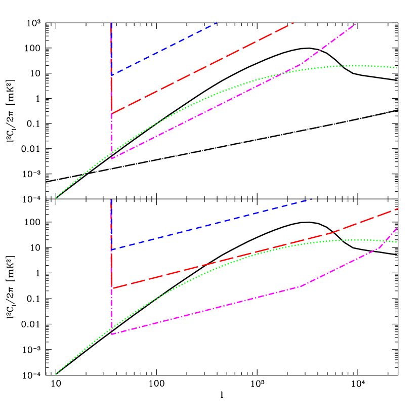
Figure 5.— Observability of the estimated 21 cm fluctuation signal. The solid black and dotted green curves in each panel are the angular power spectrum of the signal at $z=10$ (with $\Delta\nu=0.2\mbox{ MHz}$) for our toy model and for a fully neutral medium. The long dash-dotted curve in the top panel shows the estimated point source foreground signal (see text). The other curves show sensitivity estimates for three proposed experiments: PAST (blue short-dashed), LOFAR (red long-dashed), and SKA (magenta dot-dashed). The top panel shows the noise power spectrum while the bottom panel shows the error in the estimated power spectrum. We assume four weeks of continuous observations for each experiment.

Oh & Mack (2003) noted another problem related to simple contamination: if the beamsize changes with frequency, the number of foreground sources in a given beam also changes with frequency. In our language, an interferometer baseline samples slightly different $l$-modes at different frequencies. The most obvious solution is either careful beamsize control with frequency or fine coverage in Fourier-space coverage, both of which must be determined during the interferometer design. If this is not possible, an alternative method is to note that this “leakage” contamination is also highly correlated in frequency-space and can be removed with techniques similar to ours (see also Gnedin & Shaver 2003).

Note that in our estimate of the foreground removal we have assumed that the 21 cm signal between the two frequency channels is completely uncorrelated [i.e. the covariance matrix of the 21 cm signal is diagonal in equation (41)]. In reality, the off-diagonal elements of the matrix will contain the cross-correlation of the two frequency bins, $C_{l}^{21cm}(\nu_{1},\nu_{2})$. The recovered signal is proportional to $[1-C_{l}^{21cm}(\nu_{1},\nu_{2})]$. This essentially provides a minimum bandwidth for foreground removal using this technique: we need the radial separation of the two frequency bins to exceed the typical correlation length. In the example we show, we have chosen $L(\Delta\nu)\gtrsim R$, so the true signal would decrease by a small amount. However, the method we have presented uses only two neighboring frequency channels to remove the contaminants. In reality, the full bandwidth of the observation should be used in estimating the smooth component of the spectrum at each point on the sky, which will considerably improve the removal algorithm. This will allow the single-frequency signal to be isolated without significant loss from correlations between neighboring frequencies. We conclude that point-source foregrounds do not present a significant problem for these measurements provided that they are smooth in frequency space.

7. Detectability

In this section we will examine the prospects for detecting the 21 cm fluctuations. We will follow the notation of White, Carlstrom, Dragovan, & Holzapfel (1999) where the formalism used to analyze data for CMB interferometers such as the Degree Angular Scale Interferometer (DASI) and the Cosmic Background Interferometer (CBI) was presented. We note that similar sensitivity estimates have been made for the Giant Metrewave Radio Telescope by Bharadwaj & Sethi (2001) and Bharadwaj & Pandey (2003).

The measured flux in a visibility is

$$V({\bf u})={\partial B_{\nu}\over\partial T}\int d^{2}n\ \delta T_{b}({\hat{\bf n}})A({\hat{\bf n}})\ e^{2\pi i{\bf u}\cdot{\hat{\bf n}}},$$ (56)

where $A({\hat{\bf n}})$ is the primary beam and ${\partial B_{\nu}/\partial T}$ converts temperature to flux. In the Rayleigh-Jeans part of the spectrum, ${\partial B_{\nu}/\partial T}=2k_{B}/\lambda^{2}$. The Fourier wavenumber $u$ is related to $l$ by $u=l/2\pi$. We can express $\delta T_{b}({\hat{\bf n}})$ and $A({\hat{\bf n}})$ in terms of their Fourier components,

$$\delta T_{b}({\hat{\bf n}}) = \int d^{2}u\ \tilde{\delta T}_{b}({\bf u})e^{-2\pi i{\bf u}\cdot{\hat{\bf n}}}$$

$$A({\hat{\bf n}}) = \int d^{2}u\ \tilde{A}({\bf u})e^{-2\pi i{\bf u}\cdot{\hat{\bf n}}}.$$ (57)

The Fourier components $\tilde{\delta T}_{b}({\bf u})$ are essentially the same as the $a_{lm}$’s introduced earlier except that the spherical harmonic decomposition has been replaced by a Fourier decomposition, valid only over small patches of the sky that can be taken to be flat. The variance of $\tilde{\delta T}_{b}({\bf u})$ is given by the power spectrum,

$$\langle\tilde{\delta T}_{b}({\bf u}_{1})\tilde{\delta T}_{b}({\bf u}_{2})\rangle=\delta^{D}({\bf u}_{1}+{\bf u}_{2})C_{l=2\pi u_{1}}.$$ (58)

In terms of these Fourier variables the variance of the temperature is

$$\langle\delta T_{b}^{2}({\hat{\bf n}})\rangle=\int d^{2}uC_{l=2\pi u}=\int dl{lC_{l}\over 2\pi},$$ (59)

which can be compared to the exact formula,

$$\langle\delta T_{b}^{2}({\hat{\bf n}})\rangle=\sum_{l}{(2l+1)C_{l}\over 4\pi}.$$ (60)

We now calculate the averaged value of the square of the observed visibilities in terms of the power spectrum, where the average is over an ensemble of possible skies,

$$\langle|V({\bf u})|^{2}\rangle = \left({\partial B_{\nu}\over\partial T}\right)^{2}\int d^{2}u^{\prime}\ |\tilde{A}({\bf u}-{\bf u}^{\prime})|^{2}C_{l=2\pi u^{\prime}}$$ (61)

$$\approx C_{l=2\pi u}\left({\partial B_{\nu}\over\partial T}\right)^{2}\int d^{2}u^{\prime}\ |\tilde{A}({\bf u}-{\bf u}^{\prime})|^{2}.$$

If the visibility is observed for a time $t_{v}$ the averaged noise squared in each visibility is given by (Rohlfs & Wilson, 2000)

$$\langle|N({\bf u})|^{2}\rangle=\left({2k_{B}T_{sys}\over A_{dish}}\right)^{2}\ {1\over\Delta{\nu}t_{v}}$$ (62)

where $T_{sys}$ is the system temperature, $\Delta{\nu}$ is the bandwidth, and $A_{dish}$ is the area of each individual antenna in the array.

We can compare equations (61) and (62) to define the power spectrum of the noise,

$$C_{l}^{N}=\left({2k_{B}T_{sys}\over A_{dish}\partial B_{\nu}/\partial T}\right)^{2}\ {1\over\Delta{\nu}t_{v}\int d^{2}u^{\prime}\ |\tilde{A}({\bf u}-{\bf u}^{\prime})|^{2}}.$$ (63)

The result of the integral in the denominator depends on the shape of the primary beam (i.e. the beam of the individual dishes). To get an approximate answer we can use the fact that $A({\bf u})$ is different from zero in an area $d^{2}u$ and has to integrate to one, so $\int d^{2}u^{\prime}\ |\tilde{A}({\bf u}-{\bf u}^{\prime})|^{2}\sim 1/d^{2}u$. Moreover, the size of the primary beam and thus $d^{2}u$ is directly related to the area of the dishes. We can approximately use $A_{dish}=\lambda^{2}d^{2}u$. The power spectrum of the noise then becomes

$$C_{l}^{N}={T_{sys}^{2}\over\Delta\nu t_{v}d^{2}u}={T_{sys}^{2}\ (2\pi)^{2}\over\Delta\nu t_{v}d^{2}l}.$$ (64)

This is equation (17) of White et al. (1999) with the mapping $l=2\pi u$. Perhaps an easier way to understand this equation is to note that after a time $t_{v}$ the noise in the Fourier space pixel corresponding to the observed visibility is simply $\sigma_{n}^{2}=T_{sys}^{2}/\Delta\nu t_{v}$. The noise can be expressed in terms of a power spectrum using $\sigma_{n}^{2}=d^{2}uC_{l}=d^{2}l\ C_{l}/(2\pi)^{2}$.

Interferometric CMB experiments such as DASI and CBI were conducted at much higher frequencies than those in which we are interested, so the arrays were small enough that they could be rotated to compensate for the Earth’s rotation. Consequently, each pair of antennae could integrate for an arbitrarily long time on a single Fourier component of the sky. This is not feasible in the present case because the distances involved are much larger: the arrays must have baselines on the order of a kilometer. We therefore need to calculate the fraction of the total observing time $t_{0}$ that any given baseline is being observed. This fraction of time will not be uniform across the Fourier plane, and the details will depend on the element configuration.

We will make a simple estimate here assuming that the Fourier coverage is roughly uniform. For a particular maximum separation of the antennae the interferometer will cover Fourier space up to a maximum $l_{max}$. Thus, owing to the Earth’s rotation, a region of area $\pi l_{max}^{2}$ of Fourier space will be covered. At any given instant, however, only an area $N_{pairs}d^{2}l$ is being observed. Thus each visibility will be observed roughly for a time

$$t_{v} \approx t_{o}\ {N_{pairs}d^{2}l\over\pi l_{max}^{2}}$$ (65)

$$= t_{o}\ {N_{dish}^{2}d^{2}l\over 2\pi l_{max}^{2}},$$

where $N_{pairs}=N_{dish}(N_{dish}-1)/2$ and where we have assumed $N_{dish}\gg 1$. Combining equations (64) and (65) we obtain

$${l^{2}C_{l}^{N}\over 2\pi}={T_{sys}^{2}\ (2\pi)^{2}\over\Delta\nu t_{o}}\ \left({l_{max}^{2}\over N_{dish}d^{2}l}\right)^{2}\ \left({l\over l_{max}}\right)^{2}.$$ (66)

We can think of the array as a big telescope with diameter $D$, large enough to make a measurement of mode $l_{max}$ which covers a total area $A_{total}$. However, only a fraction of that area is covered with telescopes, $N_{dish}A_{dish}$. That covering fraction can also be expressed in terms of $l_{max}$ and $d^{2}l$,

$$f_{cover}\equiv{N_{dish}A_{dish}\over A_{total}}={N_{dish}d^{2}l\over l_{max}^{2}}.$$ (67)

In terms of $f_{cover}$ the noise power spectrum is,

$${l^{2}C_{l}^{N}\over 2\pi}={T_{sys}^{2}\ (2\pi)^{2}\over\Delta\nu t_{o}f_{cover}^{2}}\ \left({l\over l_{max}}\right)^{2}.$$ (68)

If one is interested in achieving maximum sensitivity at a particular scale $l$ with a fixed number of elements of a given size, it is best to pack the elements as close as possible because $l_{max}\propto D$ but $f_{cover}\propto D^{-2}$. This is achieved when the $l$ of interest is close to $l_{max}$. The signal from the “bubbles” is located somewhere in the range $l\sim 1000-10000$ so one needs an array of size $D=l\lambda/2\pi\sim 300$m - 3 km to observe it.

For realistic arrays, the distribution of telescopes will not be uniform, so the coverage in Fourier space will vary with $l$. For example, the array may have a core at the center where telescopes are closely packed and a more dilute configuration at larger separations. Thus the covering fraction for the $l$’s measured by the core of the array will be much larger than for the higher $l$’s. We can introduce a function $\tilde{f}(l)$ that encodes the geometry of the array, in terms of which

$${l^{2}C_{l}^{N}\over 2\pi}={T_{sys}^{2}\ (2\pi)^{2}\over\Delta\nu t_{o}\tilde{f}^{2}(l)}.$$ (69)

For our simple case of uniform Fourier coverage,

$$\tilde{f}(l)=f_{cover}{l_{max}\over l}.$$ (70)

The system temperature at these frequencies will be dominated by the sky brightness temperature so the figure of merit to compare different experiments is simply $\tilde{f}(l)$. We take $T_{sys}$ to be roughly $200$ K, so the noise power spectrum is approximately

$$\delta T_{n} = \left[{l^{2}C_{l}^{N}\over 2\pi}\right]^{1/2}$$ (71)

$$\sim 12\ {\rm mK}\ \left({T_{sys}\ \ 0.1\over 200K\ \tilde{f}(l)}\right)\ \left({0.4{\rm\ MHz}\ 1\ {\rm month}\over\Delta\nu\ t_{o}}\right)^{1/2}.$$

Thus, if we want an experiment to make a map with good signal to noise in a matter of weeks it needs to have $\tilde{f}(l)\sim 0.1$ on the scales of interest. Note that this noise estimate does not take cosmic variance into account. Because each observation samples only a finite region and must ultimately be compared to a statistical model of the Universe, at a certain point (when the signal to noise is of order unity in each Fourier mode), the experimental power becomes limited by the finite field of view and one is better off increasing the area of the sky being covered rather than going deeper on the same spot. We have quoted the answer for a bandwidth of order $0.4$ MHz. There is little to be gained by making the bandwidth much larger because by doing so one enters the Limber regime on the angular scales of interest (see Figure 4 and discussion thereof). Once in the Limber regime both signal and noise scale as $1/\Delta\nu$. The exact crossover into the Limber regime will depend on the sizes of the bubbles. On the other hand, if the bandwidth is much smaller than the typical correlation length of the 21 cm features, the signal will be difficult to detect as it will be confounded by the foregrounds.

If one is interested in a statistical detection of the power spectrum rather than imaging, the required observing time is significantly reduced simply because one can make several estimates of the power spectrum on scales smaller than the total field of view. The error in the power spectrum estimate is [equation (6.1)]

$${\Delta C_{l}^{21cm}\over C_{l}^{21cm}}=\sqrt{2\over N_{l}}{C_{l}^{N}\over C_{l}^{21cm}}.$$ (72)

The signal to noise increases by a factor, $\sqrt{N_{l}/2}\sim\sqrt{N_{dish}/f_{cover}}\sim\sqrt{A_{total}/A_{dish}}$. In terms of the $l$-modes sampled, $\sqrt{N_{l}/2}\sim l/l_{min}$, where $l_{min}$ corresponds to the total angular size of the field of view.

Moreover, we have included only one frequency channel in our estimate (after foreground subtraction). If the signal that one is seeking has a frequency width $\gg 1\mbox{ MHz}$, stacking channels adds even more statistical power: the number of estimates of $C_{l}^{21cm}$ goes like the number of channels used in the estimate. For example, Figure 3 shows that the power spectrum of our toy model changes relatively little over $\Delta z\sim 1$, corresponding to a frequency width of $\sim 10\mbox{ MHz}$. Thus, about 25 channels could be stacked without losing too much redshift information.

Several experiments are now being designed to have the capability to measure the 21 cm signal. One is a proposed dedicated experiment called the Primeval Structure Telescope (PAST). This instrument will have an effective area $N_{dish}A_{dish}\sim 10^{4}{\rm m}^{2}$ concentrated in a diameter $D\sim 2$ km ($l_{max}\sim 5000$). For that configuration $\tilde{f}(l)\sim N_{dish}A_{dish}/D^{2}\ (l_{max}/l)\sim 0.0024\ l_{max}/l$. Thus the instrument would require long integrations or averages over many frequency channels to detect the expected statistical signal. Note that some long baselines would also be needed to be able to remove point source contamination.

Detecting cosmic 21 cm emission is also one of the major science goals of the Low Frequency Array (LOFAR) and the Square Kilometer Array (SKA). LOFAR will have a total effective area of about $2\times 10^{5}$ ${\rm m^{2}}$ with approximately 25% of that area concentrated in a compact array of $D\sim 2$ km. For this core, $l_{max}\sim 5000$ and $\tilde{f}(l)\sim 0.016\ l_{max}/l$. The design of the SKA has not yet been fixed. Current plans call for $\sim 20\%$ of the array elements to lie in a core of $D\sim 1$ km and $\sim 50\%$ to lie within a region of $D\sim 6$ km. For the inner region, $l_{max}\sim 2500$ and $\tilde{f}(l)\sim 0.25\ l_{max}/l$ and for the outer one $l_{max}\sim 10^{4}$ and $\tilde{f}(l)\sim 0.018\ l_{max}/l$. Both of these instruments also have the advantage of very long baselines (hundreds or thousands of kilometers) that will help with point source removal and control of systematics.

Figure 5 shows some estimated sensitivity curves for each of these instruments. To construct the curves, we assumed one month of continuous observing on a single field of view. We assumed a 100 square degree field of view for each of the experiments. We have also made some assumptions about the antenna distributions in these experiments. For LOFAR, we took ($25\%,\,50\%$) to have baselines smaller than ($2,\,12$ km). For SKA, we took ($20\%,\,50\%,\,55\%$) within ($1,\,6,\,12$ km). We assumed that $\tilde{f}(l)$ varies smoothly between these points and uniform Fourier space coverage within the core. Note that our sensitivity estimates are only approximate and depend on the Fourier space coverage of the array as well as the correlation procedure.

The top panel shows the noise power spectrum; comparison to the power spectrum of the 21 cm fluctuations gives the signal-to-noise value for each measured visibility. This panel therefore shows the appropriate sensitivity for making a map. Clearly, creating images with high signal to noise on arcminute scales will be difficult and require large collecting areas (on the order of a square kilometer). Note that the slope of the sensitivity curves depend on the antenna configuration; for uniform Fourier coverage, $\delta T_{n}\propto l$. Configurations in which the coverage increases at smaller separations (i.e. the array’s covering fraction increases toward the center) have steeper slopes.

Fortunately, as noted above, a statistical measurement of the power spectrum is considerably easier. In the bottom panel we show the error on the estimated power spectrum in logarithmic $l$-bins: this is simply the noise power spectrum multiplied by $N_{l}^{-1/2}\sim l_{\rm min}/l$. The large field of view of SKA allow rather precise measurements of the power spectrum on scales from $\lesssim 1$ arcmin to $\sim 1\arcdeg$. Note also that we show the errors in the individual frequency channels. If many channels are stacked together, the errors will decrease by the square root of the number of channels (ignoring correlations between channels). In this way, PAST and especially LOFAR could also make significant detections of the power spectrum

8. Conclusions

The recent successful efforts to map anisotropies in the cosmic microwave background have determined the global properties of the Universe to high precision (e.g. Spergel et al. 2003). When combined with the highly successful paradigm for the hierarchical growth of structure (e.g. White & Rees 1978), these results imply that the evolution of the Universe on large scales is now relatively well-understood. However, on the smaller scales characteristic of individual objects, many uncertainties remain owing to our ignorance of the nature of dark matter, the lack of a full physical model for the origin of primordial density fluctuations, and our poor understanding of galaxy formation. Determining the properties and consequences of the first luminous objects at $z\sim 15-30$ may help to clarify these issues.

The evolution of the ionized part of the IGM at high redshifts provides a fossil record of the Universe at these times. In principle, the physical state of this diffuse gas constrains when and where the first luminous objects formed as well as the nature of the sources responsible for reionization. The relatively large electron scattering optical depth obtained from the WMAP observations is indicative of a complex reionization history but, by itself, does not provide unambiguous answers to the remaining questions.

In this paper, we have argued that fluctuations in 21 cm emission from the IGM can be used to measure the three-dimensional distribution of neutral hydrogen at high redshifts. Measurements of the angular power spectrum at different frequencies can be used to mitigate contamination by foreground sources that would otherwise overwhelm the 21 cm signal. Our approach is similar to that employed in analyses of CMB anisotropies, but is more general because of the frequency-dependent nature of redshifted 21 cm emission, making it possible to use 21 cm fluctuations study the evolution of reionization. We note here that the most basic kind of experiment is to seek an “all-sky” signature corresponding to a global phase transition in the neutral hydrogen (which could be reionization, reheating, or the onset of Ly$\alpha$ coupling; Shaver et al. 1999). While valuable (especially because they have much less stringent sensitivity requirements), these measurements only provide the most basic information. Moreover, they are subject to severe foreground contamination (Gnedin & Shaver, 2003) because the large scale signal varies relatively smoothly with frequency. Thus frequency differencing will not be as effective as with small-scale fluctuations. The small-scale fluctuations we have described will therefore ultimately be a better route to pursue.

Using a simple conceptual model for the morphological evolution of ionized regions, we have demonstrated how reionization imprints characteristic features into the angular power spectrum of 21 cm fluctuations. Our formulation is general, but for illustrative purposes we have adopted simplifying assumptions to emphasize salient features of our methodology. For example, in our toy model of reionization, we have ignored redshift space distortions in the 21 cm signal and neglected correlations between the density and neutral fraction fields. In future work, we will investigate the impact of these effects explicitly using semi-analytic methods and numerical simulations to show how the formalism can be adapted to account for these complications.

In principle, measurements of the type we propose can be used to distinguish between various evolutionary histories. Models with multiple epochs of reionization (e.g. Cen 2003; Wyithe & Loeb 2003) lead to a behavior in which the volume fraction of ionized gas in the universe shows a complex dependence on redshift (e.g. Figures 8 & 9 of Sokasian et al. 2003b), unlike single episodes of reionization where the trend is simpler (e.g. Figure 5 of Sokasian et al. 2003a). These differences will be imprinted onto the frequency dependence of 21 cm fluctuations of the IGM and can be discerned using the approach described here. In fact, the simple model described in §4 is only part of the story available to us through 21 cm observations. For example, the fluctuations constrain the thermal history of the IGM as well as the ionization history (see §2). If the earliest ionizing sources have hard spectra (such as quasars), we would expect the IGM to be heated rapidly, while if cool, low-mass stars are responsible for reionization, the heating would occur much closer to overlap. Another way to look at this is that the reionization history determines how much information is available to us through 21 cm fluctuations.

For instance, in a scenario with rapid heating, we will have a long epoch where density variations dominate the signal. The power spectrum of the 21 cm fluctuations is a direct tracer of the matter power spectrum. Thus, detailed measurements of this signal could provide invaluable constraints on the primordial spectrum on small scales which could tightly constrain the physics of the early Universe. In particular, because one gets many independent maps by varying the frequency, the constraints on the power spectrum obtained in this way could be significantly better than those coming from the CMB primary anisotropies. Also, 21 cm fluctuations allow one to probe the power spectrum at $z\sim 10$–$20$, an epoch inaccessible to both the CMB and galaxy surveys and a relatively large lever with which to study the growth of fluctuations. On the other hand, the 21 cm signal depends on complex physical processes (see §2) and interpreting the results will require careful modeling.

Differences in the evolutionary state of the ionized IGM also contain information about the matter power spectrum on small scales. For example, in cosmological models with reduced small-scale power, the halos hosting star-forming regions form late, delaying the ionizing effects of the first luminous objects (e.g. Somerville et al. 2003; Yoshida et al. 2003b,c). Thus, universes with a large component of warm dark matter or those in which the matter power spectrum has a running spectral index should exhibit lower amplitude fluctuations in 21 cm emission from higher redshifts than in conventional $\Lambda$CDM models.

A detailed study of 21 cm fluctuations can also constrain the nature of the sources responsible for reionization. In some scenarios, it is conjectured that reionization occurs “outside-in,” affecting voids first and high density regions later (e.g. Miralda-Escudé et al. 2000). This progression would be expected if the sources are rare, but bright. Alternatively, reionization could proceed in the opposite sense, “inside-out,” particularly if the sources are numerous, but faint (e.g. Gnedin 2000; Sokasian et al. 2003a). The former possibility would apply if quasars were the primary sources of ionizing radiation, while stars in low-mass galaxies would be more relevant to the “inside-out” scenario. The morphological appearance of the ionized gas is different in these two cases, and these differences would be reflected in the angular power spectrum of 21 cm fluctuations and how this quantity varies with frequency. In particular, the size of the H II regions at a given $x_{H}$ constrains the number density of ionizing sources. Also, if voids are ionized first the density and $x_{H}$ fields will be correlated (i.e., the neutral fraction falls first in regions that are already underdense), while the opposite is true in an “inside-out” scenario. Thus the amplitude of the brightness temperature fluctuations contains information about the process of reionization.

As we have argued in §7, the technological requirements for detecting 21 cm fluctuations from cosmic gas at high redshifts, while demanding, are within reach. In the near future, it is likely that measurements of the power spectrum of 21 cm fluctuations will reveal the physical state of the Universe at an epoch that is currently inaccessible to other observational probes.

References

- Allison & Dalgarno (1969) Allison, A. C., & Dalgarno, A. 1969, ApJ, 158, 423
- Barkana & Loeb (2001) Barkana, R., & Loeb, A. 2001, Phys. Rep., 349, 125
- Becker et al. (2001) Becker, R. H., et al. 2001, AJ, 122, 2850
- Bharadwaj & Pandey (2003) Bharadwaj, S. & Pandey, S. K. 2003, Journal of Astrophysics and Astronomy, 24, 23
- Bharadwaj & Sethi (2001) Bharadwaj, S. & Sethi, S. K. 2001, Journal of Astrophysics and Astronomy, 22, 293
- Carilli et al. (2002) Carilli, C. L., Gnedin, N. Y., & Owen, F. 2002, ApJ, 577, 22
- Cen (2003) Cen, R. 2003, ApJ, 591, L5
- Chen & Miralda-Escudé (2003) Chen, X., & Miralda-Escudé, J. 2003, ApJ, submitted, [astro-ph/0303395]
- Ciardi & Madau (2003) Ciardi, B., & Madau, P. 2003, ApJ, 596, 1
- Cohen et al. (2003) Cohen, A. S., Rottgering, H. J. A., Jarvis, M. J., Kassim, N. E., & Lazio, T. J. W. 2003, ApJ, in press [astro-ph/0310521]
- Cooray (2003) Cooray, A. 2003, astro-ph/0309301
- Couchman & Rees (1986) Couchman, H. M. P., & Rees, M. J. 1986, MNRAS, 221, 53
- Di Matteo et al. (2002) Di Matteo, T., Perna, R., Abel, T., & Rees, M. J. 2002, ApJ, 564, 576
- Fan et al. (2002) Fan, X., et al. 2002, AJ, 123, 1247
- Field (1958) Field, G. B. 1958, Proc. IRE, 46, 240
- Field (1959a) —. 1959a, ApJ, 129, 525
- Field (1959b) —. 1959b, ApJ, 129, 551
- Furlanetto & Loeb (2002) Furlanetto, S. R., & Loeb, A. 2002, ApJ, 579, 1
- Furlanetto et al. (2003) Furlanetto, S. R., Sokasian, A., & Hernquist, L. 2003, MNRAS, in press [astro-ph/0305065]
- Gnedin (2000) Gnedin, N.Y. 2000, ApJ, 535, 530
- Gnedin & Shaver (2003) Gnedin, N. Y. & Shaver, P. A. 2003, ApJ, submitted (astro-ph/0312005)
- Gruzinov & Hu (1998) Gruzinov, A., & Hu, W. 1998, ApJ, 508, 435
- Gunn & Peterson (1965) Gunn, J. E., & Peterson, B. A. 1965, ApJ, 142, 1633
- Haiman & Holder (2003) Haiman, Z., & Holder, G. P. 2003, ApJ, 595, 1
- Holder et al. (2003) Holder, G. P., Haiman, Z., Kaplinghat, M., & Knox, L. 2003, ApJ, 595, 13
- Hu (1999) Hu, W. 1999, ApJ, 522, L21
- Hu & Dodelson (2002) Hu, W., & Dodelson, S. 2002, ARA&A, 40, 171
- Hu & Holder (2003) Hu, W., & Holder, G. P. 2003, Phys. Rev. D, 68, 23001
- Hui & Haiman (2003) Hui, L., & Haiman, Z. 2003, ApJ, 596, 9
- Iliev et al. (2002) Iliev, I.T., Shapiro, P.R., Ferrara, A. & Martel, H. 2002, ApJ, 572, L123
- Kaiser (1992) Kaiser, N. 1992, ApJ, 388, 272
- Kaplinghat et al. (2003) Kaplinghat, M., Chu, M., Haiman, Z., Holder, G. P., Knox, L., & Skordis, C. 2003, ApJ, 583, 24
- Knox et al. (1998) Knox, L., Scoccimarro, R., & Dodelson, S. 1998, Physical Review Letters, 81, 2004
- Kogut et al. (2003) Kogut, A., et al. 2003, ApJS, 148, 161
- Kumar et al. (1995) Kumar, A., Padmanabhan, T., & Subramanian, K. 1995, MNRAS, 272, 544
- Limber (1953) Limber, D.N. 1953, ApJ, 117, 134
- Mackey et al. (2003) Mackey, J., Bromm, V., & Hernquist, L. 2003, ApJ, 586, 1
- Madau et al. (1997) Madau, P., Meiksin, A., & Rees, M. J. 1997, ApJ, 475, 429
- Miralda-Escudé et al. (2000) Miralda-Escudé, J., Haehnelt, M., & Rees, M. 2000, ApJ, 530, 1
- Oh & Mack (2003) Oh, S. P., & Mack, K. J. 2003, MNRAS, submitted, [astro-ph/0302099]
- Peebles (1980) Peebles, P. J. E. 1980, The Large-Scale Structure of the Universe (Princeton: Princeton University Press)
- Pen (2003) Pen, U. 2003, astro-ph/0305387
- Rohlfs & Wilson (2000) Rohlfs, K. & Wilson, T. L. 2000, Tools of Radio Astronomy (New York: Springer)
- Santos et al. (2003) Santos, M. G., Cooray, A., Haiman, Z., Knox, L., & Ma, C.-P. 2003, ApJ, in press [astro-ph/0305471]
- Scott & Rees (1990) Scott, D., & Rees, M. J. 1990, MNRAS, 247, 510
- Shaver et al. (1999) Shaver, P. A., Windhorst, R. A., Madau, P., & de Bruyn, A. G. 1999, A&A, 345, 380
- Sokasian et al. (2001) Sokasian, A., Abel, T., & Hernquist, L. 2001, NewA, 6, 359
- Sokasian et al. (2002) Sokasian, A., Abel, T., & Hernquist, L. 2002, MNRAS, 332, 601
- Sokasian et al. (2003a) Sokasian, A., Abel, T., Hernquist, L., & Springel, V. 2003a, MNRAS, 344, 607
- Sokasian et al. (2003b) Sokasian, A., Abel, T., Hernquist, L., & Springel, V. 2003b, MNRAS, submitted [astro-ph/0307451]
- Somerville et al. (2003) Somerville, R.S., Bullock, J.S., & Livio, M. 2003, ApJ, 593, 616
- Spergel et al. (2003) Spergel, D. N., et al. 2003, ApJS, 148, 175
- Springel & Hernquist (2003a) Springel, V. & Hernquist, L. 2003a, MNRAS, 339, 289
- Springel & Hernquist (2003b) Springel, V. & Hernquist, L. 2003b, MNRAS, 339, 312
- Tegmark, Taylor, & Heavens (1997) Tegmark, M., Taylor, A. N., & Heavens, A. F. 1997, ApJ, 480, 22
- Theuns et al. (2002) Theuns, T., et al. 2002, ApJ, 567, L103
- Tozzi et al. (2000) Tozzi, P., Madau, P., Meiksin, A., & Rees, M. J. 2000, ApJ, 528, 597
- Venkatesan et al. (2001) Venkatesan, A., Giroux, M. L., & Shull, J. M. 2001, ApJ, 563, 1
- White, & Rees (1978) White, S.D.M., & Rees, M. J. 1978, MNRAS, 183, 341
- White, Carlstrom, Dragovan, & Holzapfel (1999) White, M., Carlstrom, J. E., Dragovan, M., & Holzapfel, W. L. 1999, ApJ, 514, 12
- Wouthuysen (1952) Wouthuysen, S. A. 1952, AJ, 57, 31
- Wyithe & Loeb (2003) Wyithe, J. S. B., & Loeb, A. 2003, ApJ, 588, L69
- Yoshida et al. (2003a) Yoshida, N., Abel, T., Hernquist, L., & Sugiyama, N. 2003a, ApJ, 592, 645
- Yoshida et al. (2003b) Yoshida, N., Sokasian, A., Hernquist, L., & Springel, V. 2003b, ApJ, 591, L1
- Yoshida et al. (2003c) Yoshida, N., Sokasian, A., Hernquist, L., & Springel, V. 2003c, ApJ, in press [astro-ph/0305517]
- Yoshida et al. (2003d) Yoshida, N., Bromm, V., & Hernquist, L. 2003d, ApJ, submitted [astro-ph/0310443]
- Zaldarriaga (1997) Zaldarriaga, M. 1997, Phys. Rev. D, 55, 1822