Cross-Correlation Studies with CMB Polarization Maps

Abstract

The free-electron population during the reionized epoch rescatters CMB temperature quadrupole and generates a now well-known polarization signal at large angular scales. While this contribution has been detected in the temperature-polarization cross power spectrum measured with WMAP data, due to the large cosmic variance associated with anisotropy measurements at tens of degree angular scales only limited information related to reionization, such as the optical depth to electron scattering, can be extracted. The inhomogeneities in the free-electron population lead to an additional secondary polarization anisotropy contribution at arcminute scales. While the fluctuation amplitude, relative to dominant primordial fluctuations, is small, we suggest that a cross-correlation between arcminute scale CMB polarization data and a tracer field of the high redshift universe, such as through fluctuations captured by the 21 cm neutral Hydrogen background or those in the infrared background related to first proto-galaxies, may allow one to study additional details related to reionization. For this purpose, we discuss an optimized higher order correlation measurement, in the form of a three-point function, including information from large angular scale CMB temperature anisotropies in addition to arcminute scale polarization signal related to inhomogeneous reionization. We suggest that the proposed bispectrum can be measured with a substantial signal-to-noise ratio and does not require all-sky maps of CMB polarization or that of the tracer field. A measurement such as the one proposed may allow one to establish the epoch when CMB polarization related to reionization is generated and to address if the universe was reionized once or twice.

]

I Introduction

The increase in sensitivity of upcoming cosmic microwave background (CMB) polarization experiments, both from ground and space, raises the possibility for detailed studies related to reionization. The main reason for this is the existence of a large angular scale polarization contribution due to rescattering of the temperature quadrupole by free-electrons in the reionized epoch [1]. This contribution peaks at angular scales corresponding to the horizon at the rescattering surface. While such a signal has now been detected with the temperature-polarization cross-correlation power spectrum measured with first-year data of the Wilkinson Microwave Anisotropy Probe (WMAP) [2], information related to reionization from it, unfortunately, is limited. While the amplitude of the signal depends on the total optical depth to electron scattering, with an estimated value of 0.17 $\pm$ 0.04 [3], the reionization history related to this optical depth is still unknown. While slight modifications to the large angular scale polarization power spectra exist with complex reionization histories, such as a two stage reionization process advocated by Ref. [4], due to large cosmic variance associated with anisotropy measurements at few tens degree scales, one cannot fully reconstruct the reionization history as a function of redshift [5].

Given the importance of understanding reionization for both cosmological and astrophysical reasons, and the increase in sensitivity and angular resolution of upcoming CMB polarization data, it is useful to consider alternative possibilities for additional studies beyond the large angular scale signal. Under standard expectations for reionization, mainly due to UV light emitted by first luminous objects, the process of reionization is expected to be patchy and inhomogeneous [6]. This leads to fluctuations in the electron scattering optical depth and a modulation to the polarization contribution such that new anisotropy fluctuations, at arcminute scales corresponding to inhomogeneities in the visibility function, is generated [7, 8]. Even if the reionization were to be more uniform, as expected from alternative models involving X-ray backgrounds [9] and reionization via particle decays [10], density fluctuations in the electron field can modulate the polarization contribution and generate secondary anisotropies [11]. The new secondary polarization fluctuations, whether due to patchiness or density inhomogeneities, however, is hardly detectable in the polarization power spectrum given the dominant primordial polarization contribution, with a peak at arcminute scales, related to the velocity field at the last scattering surface. Thus, information related to reionization is limited from measurements that involve simply the two point correlation function of polarization or the cross-correlation between polarization and the temperature. To extract additional information one must move to a higher order and consider measurements related to, for example, the three-point correlation function or the bispectrum [12].

In this paper, we consider a potentially interesting study that has the capability to allow detailed measurements related to the reionization history. The proposed measurement involves the cross-correlation between CMB polarization maps and images of the high redshift universe around the era of reionization or its end. The existence of such a correlation arises from the fact that the polarization contribution related to reionization is generated at the same epoch as that related to the tracer field selected from high redshifts. Since the reionization contribution to polarization is generated by the scattering of the temperature quadrupole, direct cross-correlation between polarization maps and a tracer field is not useful. However, since the rescattering quadrupole correlates with CMB temperature maps, one must consider higher order statistics that also use information from CMB temperature data. We consider a possibility in the form of a three point correlation function, or a bispectrum in Fourier space, involving CMB polarization maps at arcminute-scale resolution, CMB temperature maps with large angular scale anisotropy information, and maps of the high redshift universe that trace fluctuations during the reionization and prior to reionization. Examples of useful fields include maps of the infrared background anisotropies related to the redshifted UV emission by first proto galaxies [13] and fluctuations in the 21 cm background due to the neutral Hydrogen content [14]. Additional possibilities also include maps of the $z\sim 3$ universe since one can then establish the low-redshift part of the electron scattering visibility function. Cross-correlation studies with the 21 cm background may be the most interesting possibility given that one is allowed to a priori select redshift ranges from which fluctuations arise to the redshifted 21 cm emission, based on frequency information of the observations.

The paper is organized as follows. In § II, we derive the existence of a higher order correlation between CMB temperature, polarization and a tracer field of the large scale structure that overlaps with fluctuations in the visibility function. In § III, we discuss our results and suggest that there is adequate signal-to-noise to perform such a measurements and consider several applications. We conclude with a summary in § IV.

II Calculation Method

The rescattering of CMB photons by free-electrons at redshifts significantly below decoupling, at $z\sim 1100$, leads to a polarized intensity, which in terms of the linear Stokes parameters, is

$${}_{\pm}X(\hat{\bf n}) \equiv$$ (1)

$$(q\pm iu)(\hat{\bf n}) = \frac{\sqrt{24\pi}}{10}\int drg(r)\sum_{m=-2}^{2}Q^{(m)}\;_{\pm 2}Y_{2}^{m}(\hat{\bf n})\,,$$ (2)

where the quadrupole anisotropy of the radiation field is

$$Q^{(m)}({\bf x})=-\int d\Omega\frac{Y_{2}^{m}}{\sqrt{4\pi}}\Theta({\bf x},\hat{\bf n})\,.$$ (3)

In Eq. 2, $r(z)$ is the conformal distance (or lookback time) from the observer at redshift $z=0$, given by

$$r(z)=\int_{0}^{z}{dz^{\prime}\over H(z^{\prime})}\,,$$ (4)

where the expansion rate for adiabatic CDM cosmological models with a cosmological constant is

$$H^{2}=H_{0}^{2}\left[\Omega_{m}(1+z)^{3}+\Omega_{K}(1+z)^{2}+\Omega_{\Lambda}\right]\,,$$ (5)

where $H_{0}$ can be written as the inverse Hubble distance today $H_{0}^{-1}=2997.9h^{-1}$Mpc. We follow the conventions that in units of the critical density $3H_{0}^{2}/8\pi G$, the contribution of each component is denoted $\Omega_{i}$, $i=c$ for the CDM, $b$ for the baryons, $\Lambda$ for the cosmological constant. We also define the auxiliary quantities $\Omega_{m}=\Omega_{c}+\Omega_{b}$ and $\Omega_{K}=1-\sum_{i}\Omega_{i}$, which represent the matter density and the contribution of spatial curvature to the expansion rate respectively. Although we maintain generality in all derivations, we illustrate our results with the currently favored $\Lambda$CDM cosmological model. The parameters for this model are $\Omega_{c}=0.30$, $\Omega_{b}=0.05$, $\Omega_{\Lambda}=0.65$ and $h=0.65$.

The visibility function, or the probability of scattering within $dr$ of $r$, is

$$g=\dot{\tau}e^{-\tau}=X_{e}(z)H_{0}\tau_{H}(1+z)^{2}e^{-\tau}\,.$$ (6)

Here $\tau(r)=\int_{0}^{r}dr\dot{\tau}$ is the optical depth out to $r$, $X_{e}(z)$ is the ionization fraction, as a function of redshift, and

$$\tau_{H}=0.0691(1-Y_{p})\Omega_{b}h\,,$$ (7)

is the optical depth to Thomson scattering to the Hubble distance today, assuming full hydrogen ionization with primordial helium fraction of $Y_{p}(=0.24)$. In typical calculations of CMB anisotropies, the general assumption is that the universe reionized smoothly and promptly such that $X_{e}(z\lesssim z_{ri})=1$ and $X_{e}(z>z_{ri})=0$. Such an assumption, however, is in conflict with observations, so far, involving the optical depth to electron scattering measured by WMAP and the presence of a 1% neutral fraction based on Lyman-$\alpha$ optical depths related to Gunn-Peterson troughs of the $z\sim 6$ quasars in the Sloan Digital Sky Survey [15]. To explain the WMAP optical depth and low redshift data simultaneously require complex reionization histories where $X_{e}(z)$ is not abrupt, but where reionization takes a long time [16]. Since first luminous objects are usually considered as a source of reionization, the process is inhomogeneous and patchy.

FIG. 1.: Left panel: The reionization history of the universe. Here, we consider two possibilities for the reionization process involving a smooth transition over a wide range of redshift (model A) and a model which involve a sudden transition to a fully reionized model at a reionization redshift $\sim$ 15. Right panel: The visibility function related to electron scattering in the reionized epoch, $g(z)$ (see, equation 5) for both models A and B shown above. For comparison, we also show several normalized redshift distributions of tracer fields that we consider here. These are, (a) a high redshift broad distribution, such as the one related to first proto-galaxy contributions to the IR background, (b) a high redshift, but narrow, distribution expected from the 21cm background fluctuation studies in the future, and (c) a low redshift distribution, such as the distribution of $z\sim$ 3 galaxy population. Note that 21 cm fluctuation studies allow one to choose narrow bands, such as (b), in redshift over a wide range both prior to and during the reionization process and may provide the optimal tracer field for the proposed study here.

Here, we make use of two descriptions of $X_{e}(z)$ (Fig. 1; left panel). In the first case (model A), we use a calculation based on the Press-Schechter [17] mass function and related to the reionization by UV light from the first-star formation following Ref. [18]. Here, $X_{e}(z)$ varies from a value less than 10^-1 at a redshift of 30 to a value of unity when the universe is fully reionized, at a redshift of $\sim$ 5. The reionization history is rather broad and the universe does not become fully reionized till late times, though the reionization process began at a much higher epoch. The total optical depth related to this ionization history is $\sim$ 0.17, consistent with WMAP measurements [3]. As an alternative to such a history, and to consider the possibility how different reionization models can be studied with the proposed cross-correlation analysis, we also consider a reionization history that is instantaneous at the redshift of reionization of $\sim$ 15 (model B). This alternative model could arise from reionization descriptions that involve the presence of a X-ray background or where the reionization process is associated with decaying particles, among others. While the transition to a fully reionized universe, from a neutral one, is sudden, a history such as the one shown produces a similar optical depth to electron scattering as in model A.

In Fig. 1 right panel, we show the visibility function $g(z)$ related to these two reionization histories. in model A, scattering is distributed widely given the long reionization process, while in the case of model B, scattering is mostly concentrated during the sharp transition to a reionized universe. As shown in Fig. 1, one does not expect a probe of the high-z universe, say at a redshift $\sim$ 20, to correlate strongly with polarization if the reionization process is more like model B, while a strong correlation is expected if the hypothesis related to a lengthy reionization process does in fact happen.

Now we will discuss how these reionization histories determine polarization signals in CMB both at large and small angular scales. First, we note that the polarization is a spin-2 field and can be decomposed using the spin-spherical harmonics [19] such that

$${}_{\pm}X(\hat{\bf n})=\sum_{lm}\;{}_{\pm}X_{lm}\;{}_{\pm 2}Y_{l}^{m}(\hat{\bf n})\,.$$ (8)

The multipole moments of polarization field are generally separated to ones with gradient ($E$) and curl ($B$) parity such that [20]

$${}_{\pm}X_{lm}=E_{lm}\pm iB_{lm}\,.$$ (9)

Instead of Stokes-Q and -U, one can redefine two polarization related fields $E(\hat{\bf n})$, a scalar, and $B(\hat{\bf n})$, a pseudo-scalar, such that

$$E(\hat{\bf n}) = \sum_{lm}E_{lm}Y_{l}^{m}(\hat{\bf n})\,$$ (10)

$$B(\hat{\bf n}) = \sum_{lm}B_{lm}Y_{l}^{m}(\hat{\bf n})\,.$$ (11)

The cross correlation between reionization generated polarization and a tracer field of the large scale structure is zero. This can be understood based on the fact that

$$\langle_{\pm}X(\hat{\bf n})S(\hat{\bf n}^{\prime})\rangle\propto\sum_{m}\langle Q^{(m)}S(\hat{\bf n}^{\prime})\rangle=0\,,$$ (12)

since the temperature quadrupole that rescatters at low redshifts is not correlated with the local density field. There is, however, a non-zero cross-correlation between polarization and the CMB temperature anisotropy due to the fact that the temperature quadrupole related to scattering is present in the CMB temperature anisotropy map:

$$\langle_{\pm}X(\hat{\bf n})\Theta(\hat{\bf n}^{\prime})\rangle\propto\sum_{m}\langle Q^{(m)}\Theta(\hat{\bf n}^{\prime})\rangle\neq 0\,.$$ (13)

Since this is part of the standard calculation related to the $C_{l}^{TE}$ angular power spectrum, we do not further consider it.

To the next highest order, contributions to cross-correlation arise from the fact that fluctuations in the electron field is correlated with the large scale structure. This second-order term arises from the fact that

$$g(\hat{\bf n},r)=\bar{g}(\hat{\bf n},r)\left[1+\frac{\delta g(\hat{\bf n},r)}{\bar{g}(\hat{\bf n},r)}\right]\,.$$ (14)

These fluctuations lead to a second order polarization signal that peaks at arcminute angular scales and are discussed in Ref. [7, 11]

Substituting Eq. 14 in Eq. 2 and using Eq. 8, we can write the multipole moments the polarization field, in the presence of fluctuations in the visibility function, as

$${}_{\pm}X_{lm}=-\frac{\sqrt{24}\pi}{5\sqrt{5}}(4\pi)^{2}\sum_{l_{1}m_{1}}\sum_{l_{2}m_{2}}\sum_{m_{3}}i^{l_{1}+l_{2}}$$ (15)

$$\times \int dr\bar{g}\int\frac{d^{3}{\bf k_{1}}}{(2\pi)^{3}}\int\frac{d^{3}{\bf k_{2}}}{(2\pi)^{3}}Q^{(0)}(k_{1})\delta_{g}(k_{2})j_{l_{2}}(k_{2}r)j_{l_{1}}(k_{1}r)$$ (16)

$$\times Y_{l_{1}}^{m_{1}}(\hat{\bf k}_{1})Y_{l_{2}}^{m_{2}}(\hat{\bf k}_{2})_{\pm 2}Y_{2}^{m_{3}}(\hat{\bf k}_{1})$$ (17)

$$\times \int d\Omega\;_{\pm 2}Y_{l}^{m}(\hat{\bf n})Y_{l_{1}}^{m_{1}}(\hat{\bf n})Y_{l_{2}}^{m_{2}}(\hat{\bf n})_{\pm 2}Y_{2}^{m_{3}}\,{}^{*}(\hat{\bf n})\,,$$ (18)

where, following Ref. [7], we have projected the fluctuations-modulated temperature quadrupole

$$Q_{g}^{(m)}({\bf k})=\int\frac{d^{3}{\bf k_{1}}}{(2\pi)^{3}}Q^{(m)}({\bf k}_{1})\delta_{g}(|{\bf k}-{\bf k}_{1}|)\,,$$ (19)

to a basis where the $z$-axis is parallel to the ${\bf k}$ vector such that

$$Q_{g}^{(m)}({\bf k})=\sqrt{\frac{4\pi}{5}}\int\frac{d^{3}{\bf k_{1}}}{(2\pi)^{3}}Q^{(0)}({\bf k}_{1})\delta_{g}({\bf k}_{2})Y_{2}^{m}(\hat{\bf k}_{1})\,,$$ (20)

and have simplified using the Rayleigh expansion of a plane wave

$$e^{i{\bf k}\cdot\hat{\bf n}r}=4\pi\sum_{lm}i^{l}j_{l}(kr)Y_{l}^{m\ast}({\bf k})Y_{l}^{m}(\hat{\bf n})\,.$$ (21)

Since what correlates with the polarization field is the quadrupole generated by large angular scale temperature fluctuations, to simplify, we make the assumption that the relevant anisotropies are due to the Sachs-Wolfe (SW; [21]) effect

$$\Theta({\bf x},\hat{\bf n})=-\frac{1}{3}\Phi({\bf x},\hat{\bf n})\Big{|}_{r=r_{0}}\,,$$ (22)

where $r_{0}\equiv r(z=1100)$. Note that there is a correction here related to the integrated Sachs-Wolfe (ISW) effect, but since it is present only at redshifts less than 1, when the dark energy component begins to dominate the energy density of the universe, we ignore its contribution to the quadrupole. This is a valid assumption for models of reionization with an optical depth at the level of 0.1 or more since most of the rescattering is then restricted to redshifts greater than 10 or more.

Our assumption related to large angular scale fluctuations allows us to write the quadrupole at late times, when projected to an observer at a distance $r$ through free-streaming, as

$$Q^{(0)}({\bf k},r)=-\sqrt{5}\frac{1}{3}\Phi({\bf k},r_{0})j_{2}({\bf k}r_{s})\,,$$ (23)

where $r_{s}=r_{0}-r$.

Using Eq. 22, multipole moments of the temperature map at large angular scales are

$$\Theta_{lm}=-\frac{4\pi}{3}i^{l}\int\frac{d^{3}{\bf k}}{\left(2\pi\right)^{3}}\Phi({\bf k},r_{0})j_{l}(kr_{0})Y_{l}^{m}(\hat{\bf k})\,.$$ (24)

Similarly, multipole moments of the tracer field are

$$S_{lm}=\int d\Omega\,Y_{l}^{m}\,{}^{*}(\hat{\bf n})\,S(\hat{\bf n})\,,$$ (25)

and assuming that the tracer field can be described with a source radial distribution of $W^{S}(r)$ with fluctuations denoted by $\delta_{S}$, we simplify to write

$$S_{lm}=4\pi i^{l}\int\frac{d^{3}{\bf k}}{\left(2\pi\right)^{3}}\int drW^{S}(r)\delta_{S}({\bf k},r)j_{l}(kr)Y_{l}^{m}(\hat{\bf k})\,.$$ (26)

The cross-correlation with the large scale structure exists in the form of a bispectrum between polarization-temperature-tracer fields. For this, we construct, for example, $\langle E_{l_{1}m_{1}}\Theta_{l_{2}m_{2}}S_{l_{3}m_{3}}\rangle$ and after some straightforward but tedious algebra, we write

$$\langle E_{l_{1}m_{1}}\Theta_{l_{2}m_{2}}S_{l_{3}m_{3}}\rangle=$$ (28)

$$4\pi\int dr_{1}\int dr_{2}I_{l_{3}}^{gS}(r_{1},r_{2})J_{l_{2}}^{\Phi}(r_{1})$$

$$\times \int d\Omega Y_{l_{1}}^{m_{1}}(\hat{\bf n})Y_{l_{2}}^{m_{2}}(\hat{\bf n})Y_{l_{3}}^{m_{3}}(\hat{\bf n})\,,$$ (29)

where

$$I_{l}^{gS}(r_{1},r_{2}) = \frac{2}{\pi}\int k^{2}dkg(r_{1})W^{S}(r_{2})j_{l_{3}}(kr_{2})j_{l_{3}}(kr_{1})P_{gS}(k)\,,$$ (30)

$$J_{l}^{\Phi}(r) = \int\frac{k^{2}dk}{18\pi^{2}}P_{\Phi\Phi}(k_{1},r_{0})j_{l}(kr_{0})j_{2}(kr_{s})\epsilon_{l}(kr)\,.$$ (31)

Here, $\epsilon_{l}(x)=-j_{l}(x)+j^{\prime\prime}_{k}(x)+2j_{l}(x)/x^{2}+4j_{l}^{\prime}(x)/x$ and we have defined three-dimensional power spectra related to the potential-field at the last scattering surface and the cross-power spectrum between fluctuations in the scattering visibility function and the tracer field:

$$\left<\Phi({\bf k})\Phi({\bf k^{\prime})}\right> = (2\pi)^{3}\delta^{\rm D}({\bf k}+{\bf k^{\prime}})P_{\Phi\Phi}(k)$$ (32)

$$\left<\delta_{g}({\bf k})\delta_{S}({\bf k^{\prime})}\right> = (2\pi)^{3}\delta^{\rm D}({\bf k}+{\bf k^{\prime}})P_{gS}(k)\,,$$ (33)

respectively, where $\delta^{\rm D}$ is the Dirac delta function.

In these calculations, we will described $P_{gS}(k,z)$ following the halo model [22]. At large angular scales, relevant to most of the estimates in here, $P_{gS}(k,z)=b_{g}(z)b_{S}(z)G^{2}(z)P(k)$, where $P(k)$ is the power spectrum of density fluctuations in linear perturbation theory, and $b_{g}(z)$ and $b_{S}(z)$ are large physical scale biases of these two fields taken to be independent of the scale (see, below). We use the fitting formulae of Ref. [23] in evaluating the transfer function for CDM models, while we adopt the COBE normalization to normalize the linear power spectrum [24]. This model has mass fluctuations on the $8h$ Mpc^-1 scale in accord with the abundance of galaxy clusters such that $\sigma_{8}=0.86$.

The bispectrum for the case with E-mode map is given by

$$B^{E\Theta S}_{l_{1}l_{2}l_{3}}=\sum_{m_{1}m_{2}m_{3}}\left(\begin{array}[]{ccc}l_{1}&l_{2}&l_{3}\\ m_{1}&m_{2}&m_{3}\end{array}\right)\left<E_{l_{1}m_{1}}\Theta_{l_{2}m_{2}}S_{l_{3}m_{3}}\right>$$ (37)

$$= \sqrt{\frac{(2l_{1}+1)(2l_{2}+1)(2l_{3}+1)}{4\pi}}\left(\begin{array}[]{ccc}l_{1}&l_{2}&l_{3}\\ 0&0&0\end{array}\right)b^{E}_{l_{2},l_{3}}\,,$$ (40)

where,

$$b^{E}_{l_{2},l_{3}} = 4\pi\int dr_{1}\int dr_{2}J_{l_{2}}^{\Phi}(r_{1})I_{l_{3}}^{gS}(r_{1},r_{2})\,.$$ (42)

One can simplify Eq. LABEL:eqn:b with the use of the Limber approximation. Here, we use a version based on the completeness relation of spherical Bessel functions [12]

$$\int dkk^{2}F(k)j_{l}(kr)j_{l}(kr^{\prime})\approx{\pi\over 2}d_{A}^{-2}\delta^{\rm D}(r-r^{\prime})F(k)\big{|}_{k={l\over d_{A}}}\,,$$ (44)

where the assumption is that $F(k)$ is a slowly-varying function and the angular diameter distance in above is

$$d_{A}=H_{0}^{-1}\Omega_{K}^{-1/2}\sinh(H_{0}\Omega_{K}^{1/2}r)\,.$$ (45)

Note that as $\Omega_{K}\rightarrow 0$, $d_{A}\rightarrow r$.

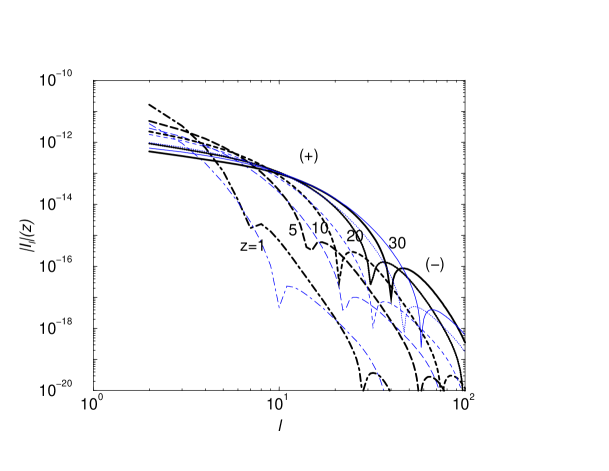
FIG. 2.: The integrals $I_{l}^{E}(r)$, with thick lines (Eq. LABEL:eqn:Il), and $I_{l}^{B}(r)$, with thin lines (Eq. 57), as a function of the multipole for several different redshift values. These mode coupling integrals oscillate between positive and negative values and we label positive/negative parts with (+)/(-). These functions captures the cross-correlation between density modulated temperature quadrupole that rescatter by an electron, at a radial distance of $r$, to form E- and B-modes of polarization and the temperature anisotropies seen by an observer at a redshift of zero or today. The multipole $l$ here is that of temperature anisotropies as seen today.

Applying this approximation to the integral in $I_{l_{3}}^{gS}$ (Eq. 31) allows us to further simplify and write

$$b^{E}_{l_{2},l_{3}} = \frac{2}{9\pi}\int drg\frac{G^{2}(r)}{d_{A}^{2}}W^{S}(r)P_{gS}\left(k=\frac{l_{3}}{d_{A}}\right)I_{l_{2}}^{E}(r)\,,$$ (46)

where

$$I_{l}^{E}(r) = \int k^{2}dkP_{\Phi\Phi}(k_{1},r_{0})j_{l}(kr_{0})j_{2}(kr_{s})\epsilon_{l}(kr)\,.$$ (47)

Similar to the bispectrum involving the E-mode map, combined with temperature and a tracer field of the high-redshift universe, one can also construct a bispectrum involving the B-mode map instead of the E-mode map. As discussed in Ref. [7], rescattering under density fluctuations to the electron distribution also lead to a contribution to the B-mode map and can be understood based on the fact that the density-modulated quadrupole generates $m=\pm 1$ components of the quadrupole which when scattered lead to B-modes. Following our earlier discussion, this bispectrum is written as

$$B^{B\Theta S}_{l_{1}l_{2}l_{3}}=\sum_{m_{1}m_{2}m_{3}}\left(\begin{array}[]{ccc}l_{1}&l_{2}&l_{3}\\ m_{1}&m_{2}&m_{3}\end{array}\right)\left<B_{l_{1}m_{1}}\Theta_{l_{2}m_{2}}S_{l_{3}m_{3}}\right>$$ (51)

$$= \sqrt{\frac{(2l_{1}+1)(2l_{2}+1)(2l_{3}+1)}{4\pi}}\left(\begin{array}[]{ccc}l_{1}&l_{2}&l_{3}\\ 0&0&0\end{array}\right)b^{B}_{l_{2},l_{3}}\,,$$ (54)

where,

$$b^{B}_{l_{2},l_{3}} = \frac{2}{9\pi}\int drg\frac{G^{2}(r)}{d_{A}^{2}}W^{S}(r)P_{gS}\left(k=\frac{l_{3}}{d_{A}}\right)I_{l_{2}}^{B}(r)\,,$$ (56)

where

$$I_{l}^{B}(r) = \int k^{2}dkP_{\Phi\Phi}(k_{1},r_{0})j_{l}(kr_{0})j_{2}(kr_{s})\beta_{l}(kr)\,,$$ (57)

where, the function that replaces $\epsilon_{l}$ in $I_{l}^{E}$ to obtain $I_{l}^{B}$ is $\beta_{l}(x)=2j_{l}^{\prime}(x)+4j_{l}(x)/x$.

In Fig. 2, we show the two quantities $I_{l}^{E,B}$ at several different values of $z$, as a function of $l$. While the function peaks at multipoles less than 4, at $z=1$, the function broadens as one moves to redshifts greater than 10 such that it is basically a constant for $l$ values up to $\sim$ 20 or more. The quantities $I_{l}^{E,B}(r)$ only depends on the background cosmology and the primordial power spectrum; with temperature anisotropy measurements and other cosmological studies, these parameters can assumed to be known. Thus, the only unknown quantity will be related to reionization through the visibility function, $g(r)$. Thus, the cross-correlation between tracer fields allow some information related to $g(r)$ be established. This includes not only whether $g(r)$ is inhomogeneous (through the detection of fluctuations), but also information on the form of $g(r)$, as a function of $r$ or binned $r$.

FIG. 3.: The angular power spectrum of CMB polarization in both the dominant gradient- or the E-mode and the B-mode. In the case of E-modes, we show the primordial contribution with the correction at large angular scales related to reionization scattering, and assuming a total optical depth to scattering of 0.17. In the case of B-modes, we neglect the primordial contribution related to gravity waves — both due to the unknown amplitude and the fact that this contribution peaks at large angular scales while the proposed correlation is related to arcminute scales — and show the important arcminute-scale signal related to lensing conversion of E- to B-modes. The long-dashed and dot-dashed curves are the secondary polarization contributions, with power in E-modes equal to B-modes, related to inhomogeneities in the reionization involving ionized fraction and the electron density field, respectively. For reionization histories related to the formation of first luminous objects, the reionization is significantly inhomogeneous and leads to a higher secondary contribution related to patchiness of the reionization when compared to fluctuations in the electron density. The two contributions also are generated at different epochs, with the patchy contribution resulting from redshifts where $0<X_{e}(z)<1$, while the density fluctuations generate contributions even when $X_{e}(z)=1$.

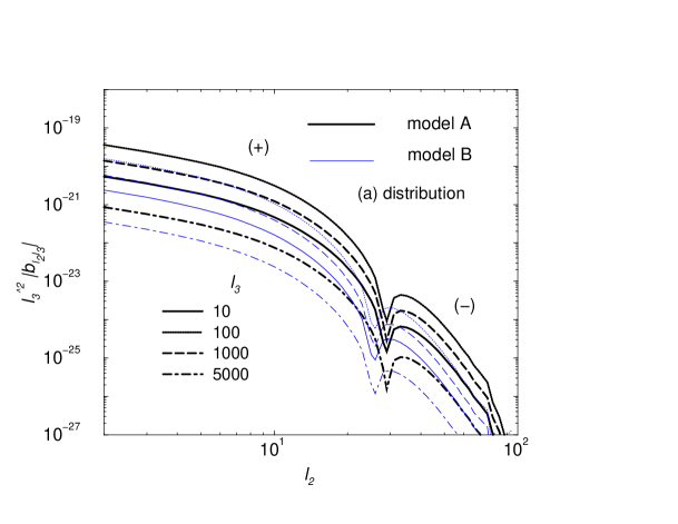
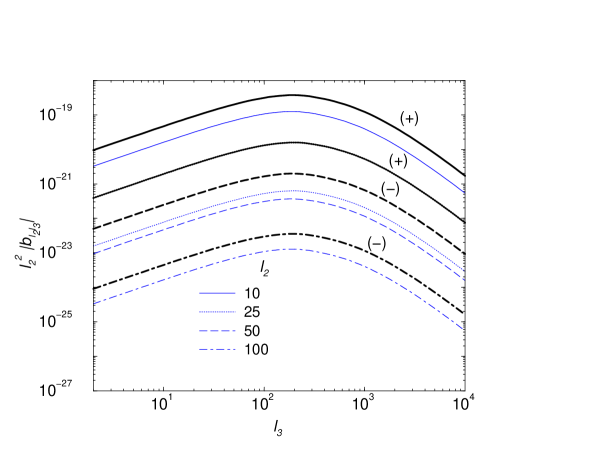
FIG. 4.: $b_{l_{2},l_{3}}$ as a function of the mutlipole for the two reionization models separated to thick (model A) and thin (model B) lines. In the top panel, we show $b_{l_{2},l_{3}}$ as a function of $l_{2}$ for several different values of $l_{3}$ while in the bottom panel we show $b_{l_{2},l_{3}}$ as a function of $l_{3}$ for several values of $l_{2}$. The curves labeled (+)/(-) are positive/negative values of this quantity. Since $b_{l_{2},l_{3}}\propto\int drf(l_{3})I_{l_{2}}$ the top panel is simply reflects $I_{l_{2}}$, as shown in Fig. 2. Here, we assume a tracer field with a distribution given by the broad high-z distribution labeled (a) in Fig. 1. As shown in the bottom panel, $b_{l_{2},l_{3}}$ values, as a function of $l_{3}$, for the two different reionization models, cannot be simply scaled by an overall normalization. Since $I_{l_{2}}$ is summed over the reionization visibility function, this is merely due to the difference in the reionization duration. The same can be inferred through Fig. 2 where, as the redshift is increased, $I_{l}$ curves shift to higher multipoles.

III Results

A Cross-correlation

It is now well known that the large scale temperature fluctuations correlate with fluctuations in polarization generated by rescattering due to free-electrons in the reionized epoch. Though there is no direct cross-correlation between polarization data and maps of the large scale structure, we suggest that the correlation between fluctuations in the large scale structure density fields and that of the electron scattering visibility function can be extracted by constructing a three-point correlation function, or a bispectrum in Fourier space, involving the large angular scale CMB temperature anisotropies, arcminute scale polarization fluctuations, and maps of the high redshift universe. The requirements for the existence of such a correlation are (1) the presence of fluctuations in the visibility function, due to density inhomogeneities or patchiness of the reionization process, and (2) overlap between the redshift distribution of scattering electrons, or the mean visibility function, and that of the tracer field.

In Fig. 1, we illustrate the basis for the proposed study. Here, we show two visibility functions related electron scattering based on two different descriptions of reionization history consistent with current estimates of the optical depth; In addition to these two, note that one can conceive a large number of reionization history models that given the same optical depth [16]. In the first scenario involving reionization by the UV light from first stars (model A), the visibility function is rather broad, but generally peaks at redshifts where $X_{e}(z)\sim 0.5$, while in the second scenario with a sudden transition to a reionized universe, scattering happens mostly during this transition.

To describe the three-dimensional cross power spectrum between the tracer field and that of the visibility function, we make use of the halo model, but concentrate only on large angular scale clustering captured by the 2-halo term. In this limit, the relevant bias factors can be described as

$$b_{i}(z)=\frac{\int_{M_{-}}^{M_{+}}dM\,M\,\frac{dN}{dM}b(M,z)}{\int_{M_{-}}^{M_{+}}dM\,M\,\frac{dN}{dM}}\,,$$ (58)

where $M_{-}$ and $M_{+}$ are the lower and upper limits of masses and $b(M,z)$ is the halo bias. We consider two possibilities for fluctuations in $g(r)$: (1) density inhomogeneities and (2) patchiness. The bias factor related to the patchy model follows from Ref. [8], while in the case of density inhomogeneities, we consider a constant bias factor of unity. This allows us to write $b_{g}(z)$ as

$$b_{g}(z)\approx 1.0+b_{X_{e}}(z)\,,$$ (59)

where $b_{X_{e}}(z)=0$ when $X_{e}(z)=1$, such that we no longer consider patchiness of the reionization when the universe is fully reionized. The bias factor related to $X_{e}$ fluctuations are described in Ref. [8] to which we refer the reader for further details; an interesting point related to this bias factor is that it is dominated by halos with temperature at the level of $10^{4}$ K and above, where atomic cooling is expected and first objects form and subsequently reionize the universe. Since what enters in the cross-correlation is the bias factor times the growth of density perturbations, in this case, the product $b_{X_{e}}(z)G(z)$ is in fact a constant [25, 26], as a function of redshift out to z of 20 or more given the rareness of halos at high redshifts.

The source bias $b_{S}(z)$, for the three tracer field distributions in Fig. 1 again involves a similar description. In the case of our low redshift distribution — curve labeled (c) in Fig. 1— we take $b_{S}(z)=1$, to be consistent with typical bias involved with galaxy fields. For the two high redshift ones, we calculate the bias following Eq. 58. For the broad high-z distribution, we take a bias factor consistent with the formation of first objects and set $M_{-}$ to be the value corresponding to virial temperatures of 10⁴K and $M_{+}\rightarrow\infty$. For the high-z narrow distribution, we assume that neutral gas is only present in halos other than those that form first objects (and, thus, assumed to be reionized). Thus we take $M_{-}\rightarrow 0$ and $M_{+}$ the value corresponding to virial temperatures of 10⁴K; note that we have taken a simple description of source bias here for both halos containing first luminous objects and halos containing neutral Hydrogen. The situation is likely to be more complicated, but our main objective is to show that there is adequate signal-to-noise for a detection of the proposed polarization-temperature-high redshift cross-correlation.

For models of extended reionization, the patchiness is more important. We illustrate this in Fig. 3 in terms of polarization power spectra. For reference, we show the primordial polarization anisotropy spectra generated at the last scattering, including the homogeneous rescattering contribution at large angular scales. The secondary scattering contributions, due to inhomogeneities, can be written as [7, 11]

$$C_{l}=\frac{3}{100}\int dr\frac{g^{2}(r)}{d_{A}^{2}}Q_{\rm rms}^{2}(r)P_{gg}\left(k=\frac{l}{d_{A}},r\right)\,,$$ (60)

where $Q_{\rm rms}^{2}(r)=\int k^{2}dk/2\pi^{2}Q^{(0)}(k,r)$. Note that the patchy polarization is generally higher [8] and may be the most important secondary polarization contribution related to scattering at arcminute scales.

Fig. 3 also illustrates why the secondary polarization contributions may be undetectable from the power spectrum alone; since the peak of the secondary contribution is at the same angular scales as the primordial power spectrum peak, with an amplitude four-orders of magnitude smaller, the cosmic variance may not allow one to extract the secondary polarization contribution easily. For comparison, in Fig. 3, we also show the expected noise power spectra related to two upcoming measurements of polarization involving Planck from space and a ground-based experiment, such as using a large-format polarization-sensitive bolometer array, with 1000 pixels, at the South Pole Telescope. We take one arcminute resolution, but limited to a sky-coverage of 4000 deg.². Other possibilities include experiments such as QUAD [27], but with slightly lower resolution (at the level of 5 arcminutes).

Given that arcminute scale polarization information is correlated with the tracer field, one does not require all-sky maps of polarization or that of the tracer field. The required temperature information, however, comes from large angular scales, as we have shown in Fig. 2 with the integral of $I_{l}^{\Phi}$. The $l$ value here corresponds to the temperature anisotropy multipole and what correlates with polarization fluctuations is the large angular scale temperature fluctuations. On the other hand, at the same time, arcminute-scale density fluctuations correlate with fluctuations in the visibility function and those responsible for secondary polarization signal. The large angular scale temperature information, fortunately, is already available from the WMAP data to the limit allowed by the cosmic variance. While CMB polarization information, at arcminute scales, will soon be avilable both from ground and space, the extent to which the proposed study can be carried out will be limited from maps of the high redshift universe.

FIG. 5.: The cumulative signal-to-noise for the detection of the temperature-polarization-high redshift bispectrum, as a function of the multipole to which information is available for the high-redshift map of a tracer field of density fluctuations.In the left panel, we make use of model A to describe reionization history and plot signal-to-noise ratios for Planck (all-sky; dotted lines), SPTpol (4000 sqr. degrees; dashed lines), and for a perfect experiment limited by cosmic variance only (all-sky; solid lines). Note that for different sky-coverages, signal-to-noise ratios scale as $f_{\rm sky}^{0.5}$. In each of these observational scenarios, we consider three possibilities related to the tracer field labeled from the top to bottom as (a), (b) and (c), respectively following Fig. 1. The bottom dot-dashed line illustrates the decrease in the signal-to-noise ratio, compared to the to the top-most solid curve, with temperature information at multipoles greater than 25; the correlation is dominated by temperature at large angular scales, and this is already available from WMAP data. In the right-panel, we compare the extent to which reionization histories related to models A and B can be distinguished. Due to the lack of scattering at redshifts $\sim$ 20 in model B, when compared to model A, we find that the cross-correlation is significantly reduced when using narrow z-band tracer fields. The planned upcoming studies at low radio frequencies involving the 21 cm background from neutral hydrogen prior to around the time of reionization may provide such narrow distributions of tracer fields.

As calculated in Eq. LABEL:eqn:ovbidefn, the bispectrum is simply proportional to the quantity $b_{l_{2}l_{3}}$. This is an integral over the radial distance of the redshift distribution functions related to the tracer field and electron scattering visibility, with their product weighted by the cross power spectrum of fluctuations between the two. To understand how this behaves, we plot $b_{l_{2}l_{3}}$ in Fig. 4 as a function of $l_{2}$ for a given $l_{3}$ (top panel) and as a function of $l_{3}$ for certain values of $l_{2}$ (bottom panel). These curves generally trace the $I_{l_{2}}$ integral shown in Fig. 2, but with an overall amplitude given by the strength of tracer field fluctuations and captured with the index $l_{3}$. Here, we show the difference between our two reionization models and using the broad high-z distribution for the tracer field. Since the reionization history related to model A is broader and expands to a higher redshift than model B, the function $b_{l_{2}l_{3}}$ for model A, for any value of $l_{3}$, expands to higher values of $l_{2}$. As shown in Fig. 2, as the redshift is increased, $I(l_{2})$ increases; since this redshift traces the reionization history, we find that in histories where scattering happens at a higher redshift than a correspondingly lower one, the contribution to the bispectrum increases as a function of $l_{2}$.

The same difference is partly responsible for the difference in overall amplitude of $b_{l_{2}l_{3}}$, but as a function $l_{3}$ with $l_{2}$ fixed (lower panel of Fig. 4). Here, the overall shape of the curve as a function of $l_{3}$, at a given $l_{2}$, is determined by the clustering strength and mainly the shape of the cross-power spectrum between fluctuations in the scattering visibility function and the tracer field. Incidentally, we also note that the amplitude changes between positive and negative values since the mode couping integral, $I_{l}$, oscillates between positive and negative values. The transition from positive to negative values is simply, again, a reflection of the reionization history. Note that the difference in curves of Fig. 4 between the two reionization models cannot simply be considered as an overall scaling of the amplitude. The bispectra can, however, be considered as a scaling along the $l_{2}$ axis for different reionization models.

B Signal-to-Noise Estimates

In order to consider the extent to which the cross-correlations can be detected and studied to understand the reionization process, we estimate the signal-to-noise ratio for a detection of the bispectrum and summarize our results in Fig. 5. The signal-to-noise is calculated as

$$\left(\frac{{\rm S}}{{\rm N}}\right)^{2}=\sum_{l_{1}l_{2}l_{3}}\frac{\left(B^{E\Theta S}_{l_{1}l_{2}l_{3}}\right)^{2}}{C_{l_{1}}^{\rm EE,tot}C_{l_{2}}^{\rm CMB,tot}C_{l_{3}}^{\rm SS,tot}}\,,$$ (61)

in the case of the E-mode related bispectrum while $E\rightarrow B$ when the B-mode bispectrum is used. Here, $C_{l}^{i,tot}$ represents all contributions to the power spectrum of the $i$th field and we write

$$C_{l}^{i,tot}=C_{l}^{i}+C_{l}^{\rm noise}+C_{l}^{\rm foreg}\,,$$ (62)

where $C_{l}^{\rm noise}$ is the noise contribution and $C_{l}^{\rm foreg}$ is the confusing foreground contribution. We refer the reader to Ref. [12] for details on the derivation related to this signal-to-noise and the relation between bispectrum and various other statistics at the three-point level, such as the skewness. Instead of focusing on these statistics, which are all reduced forms of the bispectrum either in real-space or Fourier-space, we will focus here on the bispectrum directly and consider its detection. Note that the bispectrum, as discussed in Ref. [12], capture all information at the three-point level and all other forms of statistics at this level capture only a reduced amount of information with a decrease in the signal-to-noise ratio depending on the exact statistic used and the shape of the bispectrum. While other statistics, such as skewness in real space is more easily measurable, we note that techniques now exist to construct the bispectrum reliably from CMB and large scale structure maps and have been successfully applied to understand the presence of non-Gaussianities in current data. Thus, we do not consider the measurement of the proposed bispectrum, involving CMB temperature, polarization and tracer-fields of high-z universe, to be any more complicated than what is already achieved [30].

In Eq. 62, when describing noise, in the case of CMB temperature maps, we set $C_{l_{1}}^{\rm CMB,tot}=C_{l_{1}}^{\rm CMB}+C_{l_{1}}^{\rm noise}$, where the noise contribution is related to WMAP and Planck data. Since for small values of $l_{1}$ below few hundred, $C_{l_{1}}^{\rm CMB}>>C_{l_{1}}^{\rm noise}$ in current data, we only need to consider cosmic variance. For polarization maps, we take $C_{l_{2}}^{\rm EE,tot}=C_{l_{2}}^{\rm EE}+C_{l_{1}}^{\rm noise}+C_{l}^{s}$, where $C_{l_{1}}^{\rm noise}$ is the polarization noise and $C_{l}^{s}$ is the secondary contribution to polarization anisotropy power spectrum as shown in Fig. 3. In general, $C_{l_{2}}^{\rm EE}>>C_{l}^{s}$, but $C_{l_{2}}^{\rm EE}$ is not significantly higher than $C_{l_{1}}^{\rm noise}$ for upcoming experiments such as Planck such that one must account for noise properly beyond just the cosmic variance. For the tracer field, we primarily consider only the presence of cosmic variance such that $C_{l_{3}}^{\rm SS,tot}=C_{l_{3}}^{\rm SS}$. This is due to the fact that we do not have detailed information related to detector and/or instrumental noise in certain high-z observations such as in the 21 cm background.

We can roughly estimate noise in one case involving the planned measurement of IR fluctuations due to high-z luminous sources such as the population of first propto-galaxies. We include this noise when considering cross-correlation studies with the high-z broad distribution shown in Fig. 1, since such a broad redshift distribution is expected for the high-z IR bright sources. In this case, we also include the shot-noise contribution to the tracer-field map associated with the finite density of these sources and based on models in Ref. [13]. Since the shot-noise generally peak at scales less than an arcminute, and the cross-correlation we are after is at angular scales of few arcminutes and more, we, however, find that this additional noise at small scales not to be important.

FIG. 6.: The cumulative signal-to-noise for the detection of the temperature-polarization-high redshift bispectrum using maps of the B-mode polarization and assuming a perfect experiment and a tracer field given by the (a) distribution of Fig. 1. The top dot-dashed line is for the case where the lensing B-mode power is reduced with quadratic lensing statistics (see text for details). For comparison, we also show the maximum E-mode signal-to-noise ratio. For other distributions considered, the signal-to-noise ratios scale in the same manner as shown in Fig. 5. In general, B-mode polarization maps provide a higher signal-to-noise ratio than a map of the E-mode. Though the amplitude of the foreground reionization signal is same in both E- and B-mode maps, due to a significant decrease in the primordial signal which contribute to the overall variance, the cross-correlation study is better with B-modes than E-modes as the sample variance, relative to the foreground signal, is reduced.

As shown in Fig. 5 (left panel), if the reionization history follows model A, cumulative signal-to-noise ratios range from about a few with Planck polarization maps to $\sim 10^{3}$ using perfect maps of the arcminute polarization field. These signal-to-noise ratios are substantial and are due to the fact that the correlation between temperature and the temperature quadrupole, as well as the correlation between visibility fluctuations and maps of the high-z universe, is high. As shown in Fig. 2, if scattering were to be restricted to very low redshifts, $z\sim 1$, then the correlation between temperature and the temperature quadrupole is not significant at multipoles greater than a few. On the other hand, as one moves to redshifts $\sim$ 20, this correlation is broader and spans over few tens of multipoles. Considering this, the existence of the high signal-to-noise can be understood simply as following. If we rewrite Eq. 56 for the case with a narrow redshift distribution, such as the case for high-z narrow correlation involving 21 cm fluctuations, say at a distance of $r_{x}$, we have

$$b_{l_{1},l_{2},l_{3}}\approx I_{l_{2}}^{E}(r_{x})C_{l_{3}}^{gS}(r_{x})\,,$$ (63)

where $C_{l_{3}}^{gS}(r_{x})$ is the cross-power spectrum between fluctuations in the visibility function and that of the tracer field, $S$, and is simply $C_{l_{3}}^{gS}(r_{x})\sim r_{gS}\sqrt{C_{l_{3}}^{gg}C_{l_{3}}^{SS}}$. Similarly, $I_{l}^{E}(r_{x})$ roughly scales as the cross-power spectrum between E-mode polarization and temperature, at $r_{x}$, and we can write $I_{l_{2}}^{E}(r_{x})\sim r_{ET}\sqrt{C_{l_{2}}^{EE}C_{l_{2}}^{TT}}$. The signal-to-noise ratio scales as

$$\left(\frac{{\rm S}}{{\rm N}}\right)^{2} \approx \sum_{l_{1}l_{2}l_{3}}f(l_{1},l_{2},l_{3})\frac{r_{ET}^{2}r_{gS}^{2}C_{l_{2}}^{EE}C_{l_{3}}^{gg}}{C_{l_{1}}^{\rm EE,tot}}\,,$$ (64)

where $f(l_{1},l_{2},l_{3})\sim l_{1}^{2}l_{2}^{2}l_{3}^{2}\left(\begin{array}[]{ccc}l_{1}&l_{2}&l_{3}\\ 0&0&0\end{array}\right)^{2}$. The summation over $l_{3}$, $\sum_{l_{3}}l_{3}^{2}C_{l_{3}}^{gg}$ is simply the variance related to visibility fluctuations and increases as the maximum value of $l$ over which $l_{3}$ is summed. The ratio of $C_{l_{2}}^{EE}/(C_{l_{1}}^{\rm EE,tot})$ behaves on the signal-to-noise associated with polarization measurements, especially when $l_{1}\sim l_{2}$. Thus, roughly, signal-to-noise in the correlation bispectrum, for each $l_{1}$ and $l_{2}$ mode, scales as $f_{\rm sky}^{1/2}r_{ET}^{2}r_{gS}^{2}\sigma^{2}_{gg}({\rm S}/{\rm N})^{2}_{\rm pol}$ and is determined mostly by the resolution of the polarization map and the extent to which fluctuations in the visibility function is correlated with that of the tracer field. Since $r_{ET}^{2}\sim 1$ and $\sigma_{gg}$ is $\sim$ 0.6 percent (when $l_{3}\sim 1000$), if $r_{gS}^{2}\sim 1$, one can achieve, in principle, signal-to-noise values of order $\sim$ few hundred with all-sky maps of polarization and adequate resolution in polarization down to multipoles of 1000. This, of course, assumes no noise maps in both polarization and in the tracer field and just that the noise is limited by the cosmic variance. In Fig. 5, we include instrumental and observational noise which lead to a decrease in the signal-to-noise ratio, for example, with Planck by several orders of magnitude.

In Fig. 5 (right panel), we illustrate the difference between expected signal-to-noise ratios for reionization histories involving models A and B. Here, we consider two tracer-fields involving the high-z broad distribution and the high-z narrow distribution. Fig. 1 shows the overlap between these distributions and the visibility function related to the two reionization models. This overlap, or its non-existent, helps understand differences in the bispectrum signal-to-noise ratios. In particular, we note the sharp reduction in the signal-to-noise ratio between the two models when using the narrow redshift distribution for tracer-field at high redshifts from model A to model B. This is due to the fact that most, if not all, rescattering is concentrated at redshifts below 15 in the case of model B while the tracer field is a probe of structure at redshifts of order 20.

The situation is also the same when one uses a tracer-field with a broad redshift-distribution, but limited to redshifts greater than 15. While this allows a mechanism to distinguish the extent to which two broadly different reionization models can be distinguished form one another, though they both give the same optical depth and essentially produce the same polarization signature, one can do more than this. Under the assumption that the reionization history follows an extended period, one can use tracer-fields with narrow band distributions to study the strength of the correlation as a function of redshift. This in return can be converted as a measurement of the visibility function as a function of redshift. While we have not considered such a possibility, due to the lack of information related to how well narrow band distributions can be defined at redshifts of order 15, we emphasize that 21 cm observations of the neutral Hydrogen content at high redshift may be the ideal way to approach such a reconstruction; Due to the line emission, redshift ranges can be a priori defined at observational wavelengths and such observations, when combined with CMB, may provide an interesting possibility for detailed studies related to reionization.

Instead of E-modes, as mentioned, we can also consider the B-mode for a cross-correlation study (Fig. 6). While there is no large angular scale signal related to rescattering in the B-mode map, associated with density fluctuations, at tens of arcminute scales and below, a B-mode signal exists due to modulations of the visibility function by density inhomogeneities in the ionized electron distribution. For the B-mode bispectrum, to describe noise, we take $C_{l_{2}}^{\rm BB,tot}=C_{l_{2}}^{\rm BB}+C_{l_{1}}^{\rm noise}+C_{l}^{s}$ and set $C_{l_{2}}^{\rm BB}$ as that due to gravitational lensing conversion power from E- to B-modes, as shown in Fig. 3, and ignore the presence of primordial gravity waves or tensor modes. This is a safe assumption given that such primordial contributions are expected to peak at angular scales of few degrees, while the proposed study involve tens of arcminute scale polarization.

Since the ratio of $C_{l_{2}}^{\rm sec}/(C_{l_{1}}^{\rm BB})$ is higher than that related to E-modes, one generally obtains a higher signal-to-noise ratio with an arcminute scale B-mode map when compared to a map of E-modes. The same is expected since the primordial fluctuations are smaller in B-modes than in E-modes, while the secondary contribution remains the same, the confusion generated by primary fluctuations for the cross-correlation is reduced in the case of B-modes relative to the same in E-modes. This can also be stated in terms of the reduced sample variance. There is another advantage with the use of B-mode information. Since the main confusion at arcminute scales is related to that associated with gravitational lensing confusion, one can improve the signal-to-noise ratios for the bispectrum measurement significantly, when the B-mode map is a priori cleaned with quadratic statistics or improved likelihood techniques [29]. These techniques lower the B-mode power related to lensing by more than an order of magnitude and reduces the sample variance contribution to the noise associated with the bispectrum by a similar number.

FIG. 7.: The cumulative signal-to-noise for the detection of the temperature-polarization-high redshift bispectrum, related to the gravitational lensing effect on CMB temperature and polarization anisotropies. The non-Gaussian signal is generated due to the fact that the high-redshift tracer field may correlate with the lensing deflection potential that is modifying the spatial distribution of CMB fluctuations. We show the signal-to-noise ratio for the tracer field involving the high-z broad distribution and for a perfect, Planck and SPTpol like ground-based experiment. The top curves are for the case where all information from the temperature map is included while the bottom curve, for a perfect polarization measurement, is for the case where we restrict temperature information to a multipole of 100 only. While the reionization related bispectrum is not affected by such a cutoff, due to the fact that relevant scales related to the correlation comes from large angular scale temperature anisotropy, in the case of lensing, this results in a significant reduction of this signal-to-noise. The dot-dashed line shows the signal-to-noise ratio associated with a bispectrum measurement related to lensing using the B-mode map, in addition to temperature and tracer-field information. Note the difference in scale of the ordinate between Figs. 5 and 6 and this plot.

C Contaminant Correlations

Using Figs. 5 and 6, we have argued that there is sufficient signal-to-noise for the observational measurement of the proposed correlation in the form of a bispectrum. It is also useful to consider if this bispectrum can be confused with other sources of non-Gaussianities in the CMB temperature and polarization anisotropies when correlated in the same manner with a map of the high redshift universe. The only possibility is related to the weak lensing effect on CMB anisotropies [28]. Essentially, weak lensing deflections of CMB photons lead to a correction to CMB anisotropy that depends on the temperature gradient and the deflection angle. While the temperature gradient correlates with the E-mode polarization map, the deflection angle can correlate with a map of fluctuations in the high-z universe, and generate a non-Gaussian signal related to the bispectrum.

We write the bispectrum related to this cross-correlation as

$$B^{E\Theta S}_{l_{1}l_{2}l_{3}}=\frac{1}{2}\sqrt{\frac{(2l_{1}+1)(2l_{2}+1)(2l_{3}+1)}{4\pi}}$$ (68)

$$\Big{\{}\left(\begin{array}[]{ccc}l_{1}&l_{2}&l_{3}\\ 2&0&-2\end{array}\right)F(l_{1},l_{2},l_{3})C_{l_{2}}^{\Theta E}C_{l_{3}}^{\phi S}$$

$$+ \left(\begin{array}[]{ccc}l_{1}&l_{2}&l_{3}\\ 0&0&0\end{array}\right)F(l_{2},l_{3},l_{1})C_{l_{1}}^{\Theta E}C_{l_{3}}^{\phi S}\Big{\}}\,,$$ (71)

where $F(l_{1},l_{2},l_{3})=\left[l_{2}(l_{2}+1)+l_{3}(l_{3}+1)-l_{1}(l_{1}+1)\right]$ $C_{l}^{\phi S}$ is the cross-power spectrum between lensing potentials and the tracer field and is given by

$$C_{l}^{\phi S}=\int dr\frac{W^{S}(r)}{d_{A}^{2}}W^{\phi}\left(k=\frac{l}{d_{A}},r\right)P_{\delta S}\left(k=\frac{l}{d_{A}}\right)\,,$$ (73)

where

$$W^{\phi}(k,r)=-3\Omega_{m}\left(\frac{H_{0}}{k}\right)^{2}F(r)\frac{d_{A}(r_{0}-r)}{d_{A}(r)d_{A}(r_{0})}\,.$$ (74)

Similarly, lensing induces a bispectrum related to B-modes combined with temperature information and a tracer-field. We can write this bispectrum as

$$B^{B\Theta S}_{l_{1}l_{2}l_{3}}=\frac{i}{2}\sqrt{\frac{(2l_{1}+1)(2l_{2}+1)(2l_{3}+1)}{4\pi}}$$ (75)

$$\left(\begin{array}[]{ccc}l_{1}&l_{2}&l_{3}\\ 2&0&-2\end{array}\right)F(l_{1},l_{2},l_{3})C_{l_{2}}^{\Theta E}C_{l_{3}}^{\phi S}\,.$$ (78)

(79)

In general, for high-z distributions of the tracer-field, $W^{S}(r)$ and $W^{\phi}$ do not overlap significantly. This results in a reduction in the cross-correlation between the two. Moreover, since the reionized polarization anisotropy related bispectrum can be constructed with $\Theta_{l}<100$ or so without a loss of signal-to-noise, the importance of the lensing bispectrum can be significantly reduced since limiting the lensing bispectrum to $l_{2}$ values less than 100, leads to a substantial reduction in the signal-to-noise associated with it. Even with a perfect experiment, and $l_{2}$ multipole taking same values as $l_{3}$ out to 1000 or more, the signal-to-noise ratios are not greater than few tens [28] (see, Fig. 7). With $l_{2}$ reduced to a smaller value below 100, this signal-to-noise ratio decreases substantially below a few, at most. Given that the polarization fluctuations related to bispectrum has substantially higher signal-to-noise ratios, it is unlikely that the lensing generated non-Gaussianities are a major source of concern for the proposed study related to reionization.

IV Summary

The free-electron population during the reionized epoch rescatters CMB temperature quadrupole and generates a now well-known polarization signal at large angular scales. While this contribution has been detected in the temperature-polarization cross power spectrum from WMAP data, due to the large cosmic variance associated with anisotropy measurements at relevant scales, only limited information related to reionization, such as the optical depth to electron scattering, can be extracted. The inhomogeneities in the free-electron population lead to an additional secondary polarization anisotropy contribution at arcminute scales.

While the fluctuation amplitude, relative to dominant primordial fluctuations, is small, we suggest that a cross-correlation between arcminute scale CMB polarization data and a tracer field of the high redshift universe, such as through fluctuations captured by the 21 cm neutral Hydrogen background or those in the infrared background related to first proto-galaxies, may allow one to study additional details related to reionization. This includes a possibility to recover the visibility function related to electron scattering. For this purpose, we discuss an optimized higher-order correlation measurement, in the form of a three-point function, involving information from large angular scale CMB temperature anisotropies in addition to arcminute scale polarization data. The proposed bispectrum can be measured with a substantial signal-to-noise ratio with lens-cleaned B-mode maps where the confusion related to primordial anisotropies and the arcminute scale reionization-related polarization is the least; this can be compared to other sources of non-Gaussianity in CMB data, such as due to gravitational lensing, which with the same combination of temperature, polarization, and the tracer field is at the level of at most unity in terms of the signal-to-noise ratio.

Given that the arcminute scale polarization fluctuations are correlated with fluctuations at high redshift at same angular scales, for a reliable measurement of the three point correlation function suggested here, one does not require all-sky maps of CMB polarization or that of the tracer field. This is helpful since one can obtain high signal-to-noise maps of the polarization from ground-based experiments, and in certain cases fluctuation data on certain tracers, by concentrating on limited sky-area instead of the whole sky. The required information from temperature anisotropies is at large angular scales and this information is already available to the limit allowed by the cosmic variance with WMAP data and is expected to improve with Planck in terms of the foreground confusion and separation. A study such as the one proposed may allow one to establish the epoch when CMB polarization related to reionization is generated and to address if the universe was reionized once or twice.

- [1] M. Zaldarriaga, Phys. Rev. D 55, 1822 (1997) [arXiv:astro-ph/9608050].
- [2] C. L. Bennett et al., Astrophys. J. Suppl. 148, 1 (2003) [arXiv:astro-ph/0302207].
- [3] A. Kogut et al., Astrophys. J. Suppl. 148, 161 (2003) [arXiv:astro-ph/0302213].
- [4] R. Cen, Astrophys. J. 591, 12 (2003) [arXiv:astro-ph/0210473].
- [5] M. Kaplinghat, M. Chu, Z. Haiman, G. Holder, L. Knox and C. Skordis, Astrophys. J. 583, 24 (2003); G. Holder, Z. Haiman, M. Kaplinghat and L. Knox, Astrophys. J. 595, 13 (2003); W. Hu and G. P. Holder, Phys. Rev. D 68, 023001 (2003).
- [6] e.g., see the review by R. Barkana and A. Loeb, Phys. Rep. 340, 291 (2001).
- [7] W. Hu, Astrophys. J. 529, 12 (2000) [arXiv:astro-ph/9907103].
- [8] M. G. Santos, A. Cooray, Z. Haiman, L. Knox and C. P. Ma, arXiv:astro-ph/0305471.
- [9] S. P. Oh, arXiv:astro-ph/0005262.
- [10] S. H. Hansen and Z. Haiman, arXiv:astro-ph/0305126; X. Chen and M. Kamionkowski, arXiv:astro-ph/0310473; S. Kasuya, M. Kawasaki and N. Sugiyama, arXiv:astro-ph/0309434.
- [11] D. Baumann, A. Cooray and M. Kamionkowski, New Astron. 8, 565 (2003) [arXiv:astro-ph/0208511].
- [12] e.g., in the case of CMB temperature alone, A. Cooray and W. Hu, Astrophys. J. 534, 533 (2000).
- [13] A. Cooray, J. J. Bock, B. Keating, A. E. Lange and T. Matsumoto, arXiv:astro-ph/0308407.
- [14] P. Tozzi, P. Madau, A. Meiksin and M. J. Rees, arXiv:astro-ph/9903139.
- [15] X. Fan, V. K. Narayanan, M. A. Strauss, R. L. White, R. H. Becker, L. Pentericci and H. W. Rix, arXiv:astro-ph/0111184; R. L. White, R. H. Becker, X. H. Fan and M. A. Strauss, arXiv:astro-ph/0303476.
- [16] R. Cen, Astrophys. J. 591, L5 (2003); Z. Haiman and G. P. Holder, Astrophys. J. 595, 1 (2003); J. S. B. Wyithe and A. Loeb, arXiv:astro-ph/0302297.
- [17] W. H. Press and P. Schechter, Astrophys. J. 187, 425 (1974).
- [18] X. Chen, A. Cooray, N. Yoshida and N. Sugiyama, arXiv:astro-ph/0309116.
- [19] J. N. Goldberg, J. Math. Phys. 7, 863 (1967)
- [20] M. Zaldarriaga and U. Seljak, Phys. Rev. D 55, 1830 (1997); M. Kamionkowski, A. Kosowsky and A. Stebbins, Phys. Rev. D 55, 7368 (1997) [arXiv:astro-ph/9611125].
- [21] R. K. Sachs and A. M. Wolfe, Astrophys. J. 147, 73 (1967).
- [22] A. Cooray and R. Sheth, Phys. Rept. 372, 1 (2002) [arXiv:astro-ph/0206508].
- [23] D. J. Eisenstein and W. Hu, Astrophys. J. 511, 5 (1997) [arXiv:astro-ph/9710252].
- [24] E. F. Bunn and M. J. White, Astrophys. J. 480, 6 (1997) [arXiv:astro-ph/9607060].
- [25] P. J. E. Peebles, The Large Scale Structure of the Universe (Princeton: Princeton Univ. Press) (1980).
- [26] S. P. Oh, A. Cooray and M. Kamionkowski, Mon. Not. Roy. Astron. Soc. 342, L20 (2003) [arXiv:astro-ph/0303007].
- [27] M. Bowden et al., arXiv:astro-ph/0309610.
- [28] W. Hu, Phys. Rev. D 62, 043007 (2000) [arXiv:astro-ph/0001303].
- [29] T. Okamoto and W. Hu, Phys. Rev. D 67, 083002 (2003) [arXiv:astro-ph/0301031]; M. Kesden, A. Cooray and M. Kamionkowski, Phys. Rev. D 67, 123507 (2003) [arXiv:astro-ph/0302536]; C. M. Hirata and U. Seljak, Phys. Rev. D 68, 083002 (2003) [arXiv:astro-ph/0306354].
- [30] E. Komatsu, B. D. Wandelt, D. N. Spergel, A. J. Banday and K. M. Gorski, Astrophys. J. 566, 19 (2002) [arXiv:astro-ph/0107605]; M. G. Santos et al., Phys. Rev. Lett. 88, 241302 (2002) [arXiv:astro-ph/0107588].