Magnetically Driven Accretion Flows in the Kerr Metric II: Structure of the Magnetic Field

Abstract

We present a detailed analysis of the magnetic field structure found in a set of four general relativistic 3D MHD simulations of accreting tori in the Kerr metric with different black hole spins. Among the properties analyzed are the field strength as a function of position and black hole spin, the shapes of field lines, the degree to which they connect different regions, and their degree of tangling. Strong magnetic field is found toward small radii, and field strength increases with black hole spin. In the main disk body, inner torus, and corona the field is primarily toroidal. Most field lines passing through a given radius in these regions wander through a narrow radial range, suggesting an overall tightly-wound spiral structure. In the main disk body and inner torus sharp field line bends on small spatial scales are superimposed on the spirals, but the field lines are much smoother in the corona. The magnetic field in the plunging region is also comparatively smooth, being stretched out radially by the infalling gas. The magnetic field in the axial funnel resembles a split monopole, but with evidence of frame dragging of the field lines near the poles of the black hole.

We investigate prior speculations about the structure of the magnetic fields and discuss how frequently certain configurations are seen in the simulations. For example, coronal loops are very rare and field lines connecting high latitudes on the event horizon to the disk are not found at all. Almost the entire system is matter-dominated; the only force-free regions are in the axial funnel. We also analyze the distribution of current density, with a view toward identifying possible locations for magnetic energy dissipation. Regions of high current density are concentrated toward the inner torus and plunging region. Dissipation inside the marginally stable orbit may provide a new source of energy for radiation, supplementing the dissipation associated with torques in the stably-orbiting disk body.

1 Introduction

Accretion onto black holes is potentially the most efficient form of energy generation possible; it is expected that as much as several tens of percent of the rest-mass energy of the accreted matter can become available for radiation (Novikov & Thorne 1973; but see also Gammie 1999 and Agol & Krolik 2000). The rate and character of accretion are regulated primarily by angular momentum transport, making the nature of accretion torques a fundamental problem of astrophysics. These torques result from magnetohydrodynamic (MHD) turbulence, driven by the magneto-rotational instability (MRI) (see the review by Balbus & Hawley 1998).

Large-scale numerical simulation is the best tool we have for exploring turbulent systems. The first attempts to describe the global structure of accretion onto black holes employed codes solving the equations of pseudo-Newtonian physics, i.e. Newtonian dynamics but with a gravitational potential of the Paczyński-Wiita form (Hawley 2000; Hawley & Krolik 2001, 2002; Armitage et al. 2001; Armitage & Reynolds 2003; Machida & Matsumoto 2003). For obvious reasons, these could provide only an approximate description of the dynamics, and could not explore the effects of black hole rotation.

With the construction of a fully general-relativistic three dimensional MHD code (De Villiers & Hawley 2003, hereafter DH03), it is now possible to achieve a physical description of black hole accretion that is much more complete. Using this code we have simulated accretion flows onto black holes with four different spin parameters, $a/M=0$, $0.5$, $0.9$, and $0.998$. These runs were labeled KD0, KDI, KDP, and KDE in the first paper of this series (De Villiers, Hawley, & Krolik 2003, hereafter Paper I), which presented both a detailed description of how these simulations were done and an introduction to the several distinct physical regimes found within the accretion flows. In this paper we continue our report on these simulations with a discussion of the structure of the magnetic field.

Before presenting this report, we briefly review the nature and conduct of the simulations. We adopt geometrodynamic units $G=c=1$ (Misner, Thorne, & Wheeler, 1973), and express evolution times in terms of black hole mass $M$. We also follow the convention that Greek indices represent spacetime vector and tensor components, whereas Roman indices represent purely spatial components. The simulations analyzed in this paper were evolved in Boyer-Lindquist coordinates ($t,r,\phi,\theta$) on a $192\times 64\times 192$ spatial grid ($r\times\phi\times\theta$). This grid is described as “high-resolution” in Paper I. The radial grid runs from a point just outside the event horizon (the event horizon and the inner boundary vary with $a/M$) to $r=120\,M$ using a hyperbolic cosine distribution to concentrate zones near the inner boundary. The polar angle $\theta$ runs from $0.045\,\pi$ to $0.955\,\pi$ with reflecting boundaries at the polar axis. Only the quarter plane from $0\leq\phi\leq\pi/2$ was included, with periodic boundary conditions in $\phi$. The temporal step size, $\Delta t$, is determined by the extremal light crossing time for a zone on the spatial grid, and remains constant for the entire evolution, as described in DH03. Step sizes are on the order of ${10}^{-2}\,M$ for each of the four models discussed here.

The state of the relativistic fluid at each point in the spacetime is described by its density, $\rho$, specific internal energy, $\epsilon$, $4$-velocity, $U^{\mu}$, and isotropic pressure, $P$. The relativistic enthalpy is $h=1+\epsilon+P/\rho$. The pressure is related to $\rho$ and $\epsilon$ through the equation of state of an ideal gas, $P=\rho\,\epsilon\,(\Gamma-1)$, where $\Gamma$ is the adiabatic exponent. For these simulations we take $\Gamma=5/3$. The magnetic field is described by two sets of variables. One is the constrained transport (CT) magnetic field, ${\cal B}^{i}=[ijk]F_{jk}$, where $[ijk]$ is the completely anti-symmetric symbol and $F_{jk}$ are the spatial components of the electromagnetic field strength tensor. We also define the magnetic field $4$-vector $\sqrt{4\pi}\,b^{\mu}={}^{*}F^{\mu\nu}\,U_{\nu}$, where ${}^{*}F^{\mu\nu}$ is the dual of the electromagnetic field tensor. Because the CT field is guaranteed to be divergence-free, it is the magnetic field description most readily identified with field lines. On the other hand, the magnetic field four-vector is the one most readily interpreted as a magnetic field for dynamical purposes because it arises naturally in algebraically simple forms for the stress tensor, $T^{\mu\nu}$. The magnetic field scalar is $||b||^{2}=b^{\mu}\,b_{\mu}$, and appears in the definition of the total four momentum, $S_{\mu}=(\rho\,h\ +{\|b\|}^{2})\,W\,U_{\mu}$ , where $W$ is the boost factor. Magnetic pressure is given by $P_{mag}={1\over 2}{\|b\|}^{2}$. We also define auxiliary density and energy functions $D=\rho\,W$ and $E=D\,\epsilon$, and transport velocity $V^{i}=U^{i}/U^{t}$.

For each of the four simulations, the initial conditions were basically the same: a torus with a near-Keplerian initial angular momentum distribution and pressure maximum at $r=25\,M$, containing an initial magnetic field consisting of weak poloidal field loops lying along isodensity contours inside the torus. Each simulation was run to time $8100\,M$, which is approximately 10 orbits at the initial pressure maximum. The radial boundaries permit outflow only, so the simulations have only a finite reservoir of matter to accrete. However, even in the case with the greatest integrated accretion ($a/M=0$), only 14% of the initial mass was accreted in the course of the simulation. After initial transients, the regions of the accretion flow inside the initial pressure maximum evolve into a moderately thick, nearly-Keplerian, highly-turbulent disk. This structure gives the appearance of rough statistical time-stationarity but also evolves on long timescales.

As outlined in Paper I, the quasi-steady state system is usefully divided into five regions: the main body of the disk, the coronal envelope, the inner torus and plunging region, the funnel wall jet, and the evacuated axial funnel. In this paper we make a more extensive examination of the properties and structure of the magnetic fields in these regions. Note that outside $r\simeq 25M$ (the location of the initial pressure maximum), we are not simulating an “accretion disk” at all, as material in that region moves outward as it absorbs the angular momentum taken from matter at smaller radii. For this reason, our analysis concentrates on the region $r\mathrel{\hbox{\hbox to0.0pt{\hbox{\lower 4.0pt\hbox{$\sim$}}\hss}\hbox{$<$}}}25M$, and especially on behavior in the vicinity of the innermost stable circular orbit. In §2 we examine the magnetic field strength and distribution throughout the flow. In §3 we quantify properties of the field geometry, and in §4 we determine where field dissipation would likely be important. Section 5 summarizes our findings.

2 Distribution of Magnetic Pressure

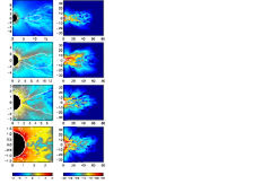
Figure 1: The azimuthally-averaged magnetic pressure, $\langle{1\over 2}\|b\|^{2}\rangle$, at $t=8080\,M$ normalized to the maximum initial gas pressure, $P_{max}$, in simulations with $a/M=0$ (first row from top), 0.5 (second row), 0.9 (third row), and 0.998 (fourth row). The left column shows the region inside $r=3\,r_{ms}$, plotted on a logarithmic scale that emphasizes the increasing dominance of magnetic pressure with black hole spin in the innermost region of the computational domain. The right column shows the main body of the disk, in a color scale that emphasizes the dominance of gas pressure in the disk body (the upper color ranges are saturated here). Three azimuthally-averaged gas pressure contours are also shown, $\langle P_{gas}\rangle$, scaled to the initial pressure maximum, $0.1\,P_{max}$ (dotted line), $P_{max}$ (solid line), $10\,P_{max}$ (dashed line).

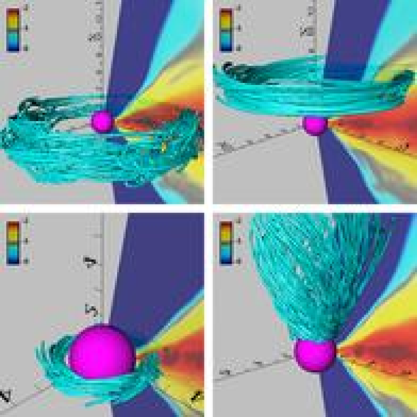
Figure 6: Sample field lines in four regions of the $a/M=0.9$ simulation. Upper left panel is the disk body (i.e., $0.45\pi<\theta<0.55\pi$, $r_{o}=10M$); upper right is the corona ($0.32\pi<\theta<0.37\pi$, $r_{o}=10M$); lower left is the plunging region ($0.475\pi<\theta<0.525\pi$, $r_{o}=2M$); lower right is the axial funnel ($0.1\pi<\theta<0.2\pi$, $r_{o}=5M$). All four are at $t=7760M$. Background colors are contours of $\log(\rho)$, calibrated by the color-bar.

The late-time structure of the magnetic scalar $||b||^{2}$ (whose physical identification is relatively simple in the context of the fluid frame–it is twice the magnetic energy density there) and its distribution in the accretion flow are found in Figure 1, which shows color contours of the azimuthal-average, $\langle{1\over 2}\|b\|^{2}\rangle$ at $t=8080\,M$ for all four simulations. The magnetic pressure is expressed in units of the initial maximum gas pressure in each simulation to permit comparison across models. (The initial gas pressure maximum increases with increasing black hole spin.) Gas pressure contours (at $t=8080\,M$) are shown as white lines in order to locate the inner torus (left panels) and the main disk body (right panels). The gradual thickening of the inner torus with increasing black hole spin is highlighted by the gas pressure contours. The left panels show that the magnetic pressure is greatest on the top and bottom surfaces of the inner torus, and that the regions of greatest magnetic pressure overlie regions where the gas pressure abruptly drops. In the funnel region, the magnetic and gas pressure profiles are very nearly circular, though magnetic pressure is dominant in this region. Although the magnetic pressure distribution looks irregular, the total pressure, gas plus magnetic, is relatively smooth; total pressure is predominantly cylindrical in distribution outside the funnel and spherical within (see fig. 6 of Paper I). Figure 1 shows that, near the black hole, magnetic pressure tends to increase with black hole spin. Near $r=5\,M$, the typical magnetic pressure grows by roughly an order of magnitude from $a/M=0$ to $0.998$; near the inner radial boundary, the magnetic pressure increases by close to two orders of magnitude from zero to maximal spin. This stands in contrast to the magnetic pressure in the main disk body at large radii ($r>30\,M$), which does not vary much with spin. Figure 1 also shows that magnetic pressure diminishes rapidly both with height above the disk surface and with increasing radius. Gradients in magnetic pressure are very large: in just a few gravitational radii outside the inner boundary, the pressure falls by 1–2 orders of magnitude. The magnetic pressure averaged over radial shells falls roughly as $r^{-3}$ from the inner radial boundary to the outer.

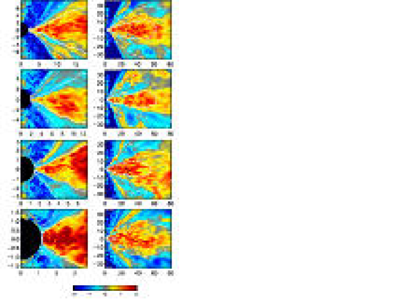
Figure 2: The azimuthally-averaged ratio of gas to magnetic pressure, $\beta=\langle P\rangle/\langle{1\over 2}\|b\|^{2}\rangle$, at $t=8080\,M$ in simulations with $a/M=0$ (first row from top), 0.5 (second row), 0.9 (third row), and 0.998 (fourth row). The left column shows the region inside $r=3\,r_{ms}$, the right column shows the main disk body; all are plotted on the same logarithmic scale. Three azimuthally-averaged density contours are also shown, $\langle\rho\rangle$, scaled to the initial pressure maximum, $0.1\,\rho_{max}$ (solid line), $10^{-2}\,\rho_{max}$ (dotted line), $10^{-3}\,\rho_{max}$ (dashed line).

The spatial relation between gas and magnetic pressures is shown in Figure 2, which presents the ratio of azimuthally-averaged gas pressure to magnetic pressure, $\beta\equiv\langle P\rangle/\langle{1\over 2}\|b\|^{2}\rangle$ (see also fig. 8 in Paper I). The main disk body and inner torus show up quite clearly in this figure since $\beta$ is greater than unity everywhere in these regions. In the dark red regions of the disk body $\beta$ can be much higher, as high as $\sim 1000$ in some locations, although it is generally lower, with a mass-weighted shell-average value of $\beta\simeq 10$–100 at all radii within the main disk body. In the inner torus and plunging region, $\beta$ tends to smaller values with decreasing radius for the $a/M=0$, 0.5, and 0.9 simulations, but remains elevated in the $a/M=0.998$ simulation, whose plunging region is both very compressed radially in Boyer-Lindquist coordinates and not well-resolved in our simulation. For all but the $a/M=0.998$ simulation, the mass-weighted mean that is 10–100 in the disk body drops to $\simeq 2$–6 near the inner radial boundary, while the volume-weighted mean $\beta$ falls from $\sim O(10)$ near $r_{ms}$ to 0.3–1 at the inner boundary. This decrease is not evenly distributed, however. Through the inner torus to the plunging region, the density contours focus toward the equatorial plane and contours of elevated $\beta$ tend to follow. Although the aspect ratio ($H/r$) of gas pressure-dominated material narrows in the plunging region, in the equatorial plane itself $\beta$ remains larger than unity all the way to the inner radial boundary. Figure 1 showed a relationship between magnetic pressure near the black hole and the spin of the black hole. Figure 2 shows that there is no comparable trend in $\beta$. Rather, as the black hole spins faster, the gas pressure and density in the inner disk become larger relative to the mass stored in the outer disk, and the magnetic pressure grows proportionately.

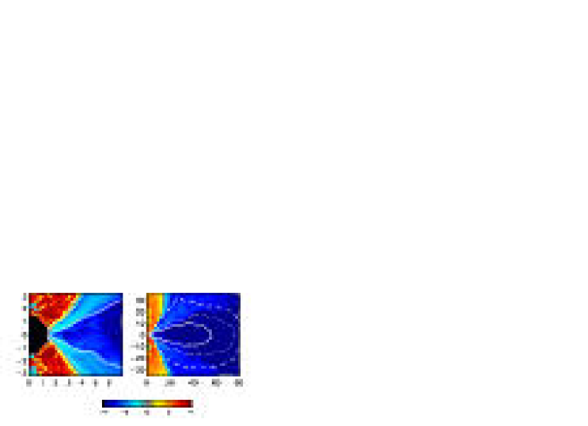
Figure 3: The azimuthally-averaged ratio of magnetic pressure to enthalpy, $\langle{1\over 2}\|b\|^{2}/(\rho\,h)\rangle$, at $t=8080\,M$ for the simulation with $a/M=0.9$. The left panel shows the region inside $r=3\,r_{ms}$, the right panel shows the main disk body; both are plotted on the same logarithmic scale. Three azimuthally-averaged density contours are also shown, $\langle\rho\rangle$, scaled to the initial pressure maximum, $0.1\,\rho_{max}$ (solid line), $10^{-2}\,\rho_{max}$ (dotted line), $10^{-3}\,\rho_{max}$ (dashed line). Images from the other three simulations are very similar.

In the coronal envelope $\beta$ is of order unity; the funnel wall jet and other outflows within the corona have $\beta>1$. Generally, $\beta$ decreases with increasing distance away from the midplane. More than two density scale-heights above the plane, $\beta\sim 0.1$ in most places. Because of field buoyancy one expects the corona to be significantly magnetized. The local stratified simulations of Miller & Stone (2000) found $\beta\sim 10^{-2}$ in the corona, but in their simulation there was relatively little mass outflow, due to the isothermal equation of state and the local disk approximation. In our simulations there is considerable outflow from the inner, hot portion of the disk into the corona, which helps to maintain $\beta$ at more modest levels. The exception, naturally enough, is the axial funnel which is magnetically dominated and has $\beta\ll 1$. The centrifugal barrier effectively prevents any significant flow of disk material into this region. The funnel does, however, contain regions of anomalously elevated $\beta$, due to shock heating of the tenuous funnel gas, which tends to enhance the pressure of the gas while its density remains extremely low. The final region of interest, the funnel-wall jet, is a region defined by two properties: the gas is unbound ($h\,U_{t}<-1$) and outbound ($S_{r}>0$) (see Paper I). Although the jet contours are not explicitly shown in Figure 2 (see figs. 3 and 10 of Paper I), they occupy a narrow band with $\beta\simeq 0.3$ that lies between the substantially lower values typical of the axial funnel and the higher values of the corona; the jet lies poleward of the extended high-$\beta$ radial streaks that stand out in the right panels. More analysis of the funnel-wall jet and the lower density outflow within the axial funnel will be provided in a subsequent paper in this series.

Another measure of the relative importance of the magnetic field is given in Figure 3 which shows $\langle{1\over 2}\|b\|^{2}/\rho\,h\rangle$, the azimuthally-averaged point-wise ratio of magnetic pressure to enthalpy. When the ratio is much greater than unity, the gas’s inertia is of minor importance to the dynamics; this state is often called “force-free” (e.g., Blandford 2002). This figure clearly distinguishes the axial funnel, the main disk body, and the coronal envelope. It is clear that nowhere in the main disk body, corona, inner torus, or plunging region is the force-free condition met. In the main disk body and most of the inner torus, the ratio is very small, typically $\sim 10^{-4}$ in the main disk body, rising to $\sim 10^{-2}$ in the inner torus and plunging region. The ratio ranges from $10^{-1}$ to 1 in the outer layers of the inflow through the plunging region (compare the prediction in Krolik 1999 that $\|b\|^{2}/\rho\sim 0.1$–1 in the most relativistic portion of the plunging region). In the axial funnel, the only region where the force-free condition is met, the ratio ranges from $\sim 100$ to 1000.

It should be noted that the GRMHD code was designed primarily for regions where the matter inertia is nonnegligible. The code employs a density and energy floor that allows a dynamic range of about seven orders of magnitude in these variables. The code also places a ceiling on the Lorentz factor $W$ ($W_{ceiling}=4$). In practice these limits come into play only at certain times within the axial funnel, which renders the accuracy of the dynamical properties within the funnel somewhat uncertain. For this reason we focus mainly on the general features of the field strength and topology in the funnel, and give less weight to detailed calculations of energy or energy flux there.

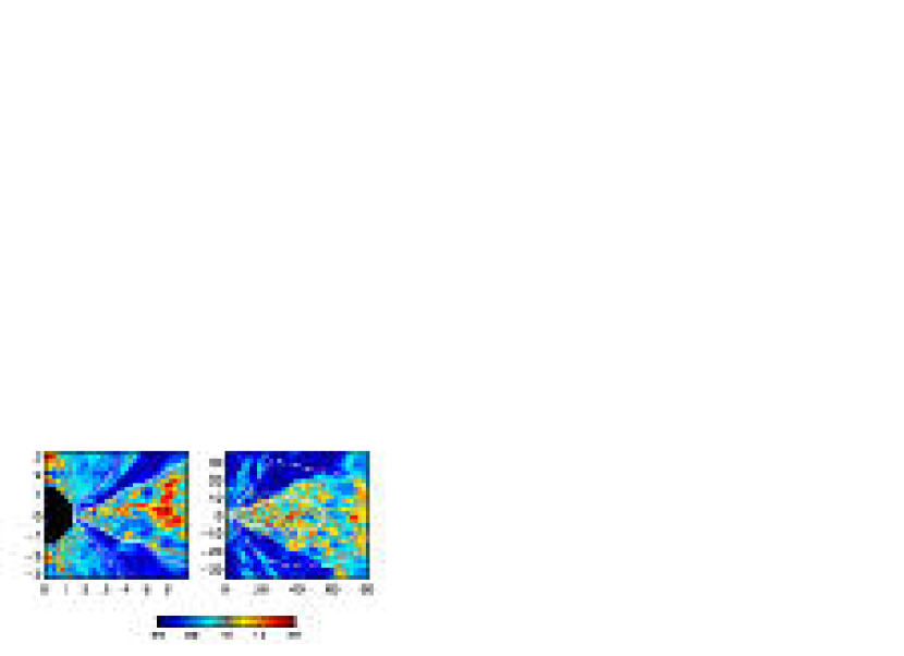
Figure 4: The fractional fluctuation in azimuth for $\|b\|^{2}$ at $t=8080\,M$ in the simulation with $a/M=0.9$. The left panel shows the region inside $r=3\,r_{ms}$, the right panel shows the main disk body; both are plotted on the same linear scale. Images from the other three simulations are very similar.

Azimuthally-averaged representations do not convey the entire picture. In Figure 4 we plot the fractional rms fluctuation level in magnetic energy density relative to its azimuthal mean in the $a/M=0.9$ simulation at $t=8080\,M$. The rms fluctuation is defined for a quantity $f$ by (Hawley & Krolik 2001)

$${\delta f\over f}\left(R,\theta\right)={1\over\langle f\rangle_{\phi}}\left\{{1\over 2\pi}\int\,d\phi\,\left[f-\langle f\rangle_{\phi}\right]^{2}\right\}^{1/2},$$ (1)

where ${\langle f\rangle}_{\phi}$ refers to the azimuthal average at fixed $R$ and $\theta$ of the quantity $f$. Fluctuations in field strength can be very large, and large fluctuations clearly delineate the main disk body and inner torus. In the $a/M=0.9$ simulation the fractional rms fluctuation level in magnetic energy density relative to its azimuthal mean ranges from 0.8–2.0 within the disk. On the other hand, both the plunging region and the corona are far more regular: the fractional rms fluctuations in both zones drop to typically 0.1–0.3. These characteristic fluctuation levels are independent of black hole spin.

Figures 1—4 show clearly that the different regions of the accretion flow have quite different magnetic characteristics. The funnel is magnetically dominated, and nearly force-free. In contrast, the main disk body and inner torus are gas pressure dominated, but their evolution is nevertheless controlled by the Lorentz forces in the MHD turbulence. The inner edge of the disk is a region where the inflow becomes increasingly magnetized. The corona is mixed; while on average the magnetic and gas pressures are comparable, the magnetic pressure has a larger effective scale height, and there are distinct regions where one or the other is dominant. Nowhere, however, does the corona approach the force-free limit.

3 Field Geometry

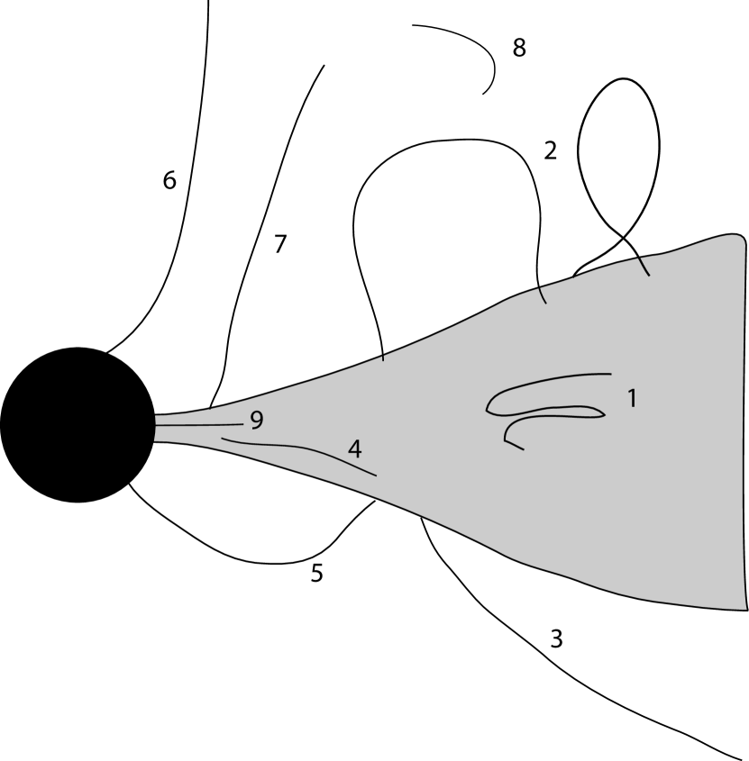
Figure 5: Schematic diagram (after Blandford 2002) showing possible magnetic linkages between different regions of the accretion flow and the black hole.

Magnetic fields have directions, of course, in addition to magnitudes, and the directions may be visualized in terms of field lines. The overall geometry of the magnetic field is important, since field lines can link together different regions of the flow in a way that is not possible by hydrodynamics alone. A convenient way to summarize the possibilities is in terms of a modification of the field line categorization introduced by Blandford (2002), who listed seven generic varieties of field lines in the vicinity of an accreting black hole. We adopt this list, but modify some of the definitions and include two additional types (see Fig. 5), as follows:

1. tangled field internal to main disk,

2. loops connecting different parts of the disk through corona,

3. open field lines emerging from the main disk,

4. field lines connecting the gas inside the plunging region to the main disk,

5. high latitude field loops connecting the black hole to the main disk,

6. open field lines from the black hole out through the funnel,

7. open field lines from the plunging region to an outflow,

8. largely toroidal field filling the corona,

9. field lines connecting the black hole to the disk through the plunging region.

We expect that the presence or absence of some of these field line types will be largely independent of the specific assumptions of a given simulation. For example, twisted field loops within the disk body (type 1) are the generic result of the MRI. Similarly, if there is accretion from the disk body into the plunging region, it is very hard to avoid creating field lines linking those two regions (type 4); the only issue is how far they extend and the field intensity associated with them. Toroidal coronal field (type 8) also appears hard to avoid whenever field is ejected into the corona. On the other hand, field line configurations such as type 2 may be more problematic. Such extended field loops have been suggested as a possible origin of high-energy emission from accretion disks. By analogy with events in the Solar corona, it is thought that the footpoints of magnetic field lines in the corona may be twisted in opposite directions by orbital shear, leading to reconnection (e.g., Blandford 2002) and a flare. But do such field configurations arise naturally in a turbulent disk?

Field line configurations such as types 5, 6, and 9 are of particular interest as they offer the possibility of extracting rotational energy from the black hole. Whether or not there are field lines connecting the accretion flow or the black hole’s event horizon to infinity bears directly on the issue of jet formation. The answers could depend on specific conditions of the accretion flow. For example, in these simulations we supposed that all field lines in the initial state were closed within the initial torus of matter. Thus, any field lines linking the disk to infinity must be created as a consequence of an outflowing wind or jet. The existence of winds and jets, and where they originate may, however, be very sensitive to the initial conditions and the detailed thermodynamics of the accretion flow. Another possibility is that accretion flows drag in field lines from large radius, thereby maintaining a connection between the accreting matter and infinity. Whether flows of this type exist is a matter of conjecture and debate (e.g., Bisnovatyi-Kogan & Ruzmaikin 1976; Thorne et al. 1986; Lubow et al. 1994).

In this section we examine the overall geometry and global connectivity of the magnetic field in these simulations. We begin by displaying the general shape and character of the field lines. Next we attempt to describe quantitatively the degree to which field links different regions of the flow, as well as the tangling of the field at small scales. We organize the discussion according to the five flow regimes identified in Paper I and the generic field topologies given in Figure 5.

3.1 Field Line Shapes

To generate field line plots, we compute integral curves for which the tangent vector at each point on the curve is parallel to the local magnetic field. In many circumstances it might be desirable to describe the field lines in the fluid frame (using the $b^{\mu}$ code variables) because in some respects that is the most physical way to view them (see DH03 for a detailed discussion of the fluid-frame variables). However, the most direct way to trace these lines is to use the CT-variables, ${\cal B}^{i}$, in the Boyer-Lindquist coordinates (i.e., work directly in the coordinate frame). The CT variables are guaranteed to be divergence-free, and have a direct relationship to the electromagnetic field strength tensor (DH03). In view of these considerations, we define the local tangent vector,

$${dx^{i}\over d\lambda}\equiv{\cal B}^{i},$$ (2)

where $x^{i}$ are position vector components on the field line in the coordinate frame and $\lambda$ is some parametrization of the curve. Taking the norm of the magnetic field,

$$\|{\cal{B}}\|^{2}=\gamma_{ij}\,{\cal B}^{i}\,{\cal B}^{j}$$ (3)

where $\gamma_{ij}$ is the spatial sub-metric, we can rewrite this expression using (2) to obtain

$$\|{\cal{B}}\|^{2}=\gamma_{ij}{\,dx^{i}\,dx^{j}\over d\lambda^{2}}$$ (4)

This allows us to normalize (2) to the local proper length of the vector field,

$${dx^{i}\over ds}\equiv{{\cal B}^{i}\over\|{\cal{B}}\|}$$ (5)

where $ds=\sqrt{\gamma_{ij}\,dx^{i}\,dx^{j}}$. This set of first-order differential equations is integrated with a Runge-Kutta-Gill method using a discrete step length ($ds\rightarrow\Delta s$) that is kept fixed ($\Delta s=0.01\,M)$. The integration for each field line is begun at a starting point $(r_{o},\theta_{o},\phi_{o})$ and continued for a distance $s^{\prime}=r_{o}$ to either side of the starting point, where $s^{\prime}$ is the nominal flat-space length, i.e., $(ds^{\prime})^{2}=dx^{i}\eta_{ij}dx^{j}$. In principle, a fourth-order Runge-Kutta scheme has an error that scales as $(\Delta s)^{5}$. However, in this case, because evaluations of the right hand side of the differential equation depend on interpolations in gridded data, the error scales as $(\Delta s)^{3}$. The fractional accumulated error in the field line’s coordinates after an integration spanning $s^{\prime}=r_{o}$ should then be $\sim 10^{-5}(r_{o}/M)^{-5/2}(l/r_{o})^{-3}$, where $l$ is the physical bending scale. To keep this error to less than one grid cell requires that $l/r_{o}\mathrel{\hbox{\hbox to0.0pt{\hbox{\lower 4.0pt\hbox{$\sim$}}\hss}\hbox{$<$}}}0.1(r_{o}/M)^{-1}$, hence the conservative choice in step size $\Delta s$. To visualize these field lines, we take the output of the integrator, which consists of a list of grid-space coordinates for each field line, and render these using a coordinate mapping from the Boyer-Lindquist ($r,\theta,\phi)$ triple onto a 3D visualization grid.

We begin our description of the field geometry with the main body of the disk, which consists, as anticipated, of turbulent, tangled toroidal fields (type 1). In the main disk body, the field geometry is controlled by two effects: orbital shear and turbulence. The former continually draws out radial field into azimuthal, while the latter twists the field in all directions on scales smaller than the local disk thickness. The resulting field line shapes are clearly shown in Figure 6. For the most part, the field lines wrap around the disk azimuthally as tightly-wound spirals, but there are numerous small twists and tangles. The magnetic field geometry is qualitatively the same for all black hole spins.

In the corona, the field is generally much more regular, and at times is almost purely azimuthal. Field-line category 8 prevails here. There are almost no tangles; adjacent field lines run very nearly parallel to one another. We must qualify this statement by acknowledging that we can examine only selected timesteps from a full simulation and that there is variation with time. For example, there are some sampled time steps in which the field in the corona more nearly resembles the field in the main disk body as shown in Figure 6, presumably due to the passage of magnetic pressure bubbles through the corona, a feature clearly seen in animations of the density variable, $\rho$. More generally, however, poloidal field loops (type 2) appear only very rarely in the corona. When they do, it is near the surface of the disk, where small scale turbulent field structures emerge from the disk body. In the disk body, the MRI maintains turbulence, and the energy density of turbulent fluid motions is comparable to or greater than the energy density in magnetic field. In the corona, on the other hand, the energy density of the magnetic field is generally greater than the energy density in random fluid motions, so the field adopts a shape primarily governed by equilibrating magnetic forces, subject to the constraint imposed by the large-scale orbital shear.

The inner part of the disk consists of the inner torus (where gas pressure reaches a local maximum) and the plunging region. The plunging region lies inside the turbulence edge (Krolik & Hawley 2002), that is, the point where the net inflow speed becomes greater than the amplitude of the turbulent motions rather than the other way around. In the plunging region, the field structure is intermediate in character between the disk body and the corona. Because inflow starts to dominate over turbulent fluctuations, the field is primarily controlled by relatively smooth stretching of field lines. Frame-dragging also helps in this regard. However, complete inflow dominance is not achieved until the flow reaches deep into the plunging region. In the $a/M=0.9$ simulation, the innermost stable circular orbit is at $2.32\,M$, at least a small amount of tangling persists throughout the plunging region, while in the $a/M=0.998$ simulation (not shown), where the plunging region is poorly resolved (Paper I), extensive tangling remains down to the inner boundary. Field-line types 4 and 9 predominate in this region, as the plunging region is linked magnetically to both the main body of the disk and the inner boundary of the simulation.

The magnetic field in the axial funnel is created in the initial accretion event when relatively strong field lines first reach the horizon. Material drains off the field lines and they rapidly expand out from the equator to fill the funnel. Once established, these field lines remain largely unchanged through the remainder of the simulation, and in polar force balance with the corona. These are field lines of type 6, a split-monopole configuration with loosely-wound helices. The dominant component is radial, but there is an azimuthal component that increases with black hole spin and proximity to the black hole. The specific angular momentum of material in this region is 2–3 orders of magnitude smaller than in the nearby disk, so nearly all the rotation is due to frame-dragging. Conversely, at increasing distances from the hole, the funnel field lines become almost purely radial. Because the angular momentum barrier prevents any matter located initially in the torus from finding its way into the axial funnel, there are almost no field line connections linking any part of the disk to the outflow. There are likewise no field lines that start at high-latitude points on the inner radial boundary, pass through the axial funnel, and lead to the disk body. That is, field lines of types 5 and 7 are entirely absent.

The field lines in the funnel-wall jets (not shown) resemble those of the axial funnel, except that they are more tightly wound, considerably more so for the high-spin simulations, $a/M=0.9$ and 0.998. This is consistent with the observations made in Paper I that the gas in the funnel-wall jets has specific angular momentum comparable to the value at the injection points, the surface of the inner torus.

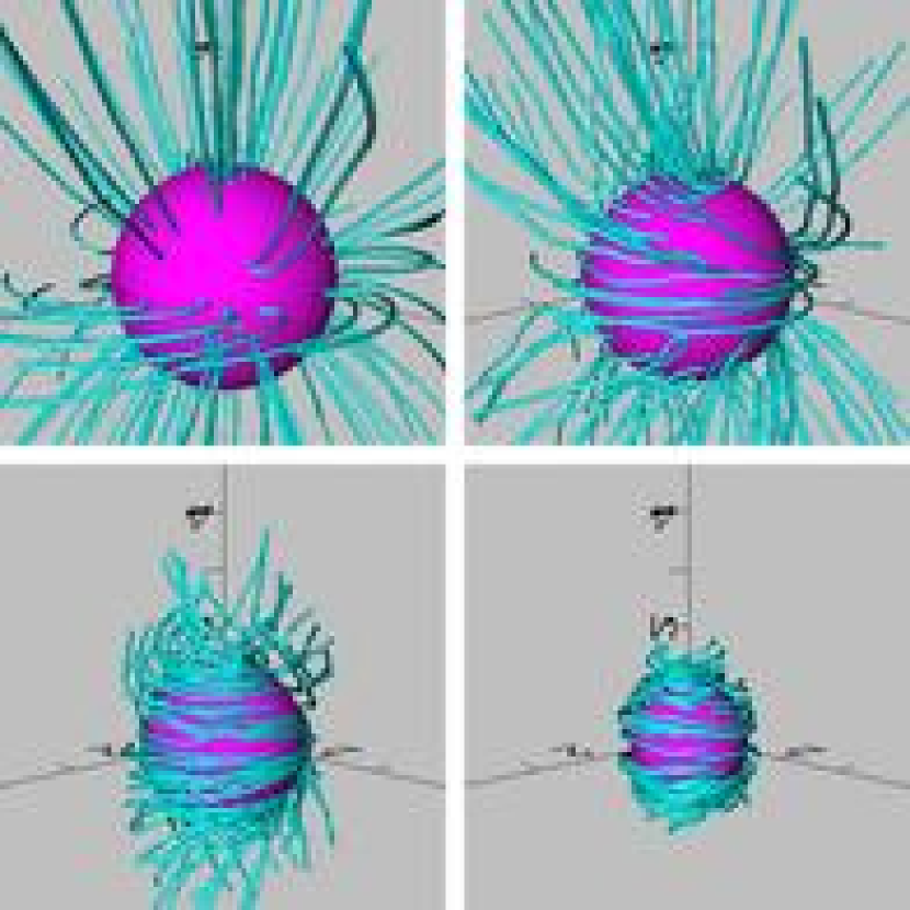
Figure 7: Sample field lines threading the innermost radial boundary in simulations with $a/M=0.$, 0.5, 0.9, and 0.998.

The effect of frame dragging on the field lines is especially prominent at the smallest radii, just outside the event horizon. Figure 7 makes this point dramatically. When $a/M=0$, field lines threading the event horizon outside the equatorial plane are almost perfectly radial. Those passing through the horizon in the plane are swept back azimuthally because they are being carried in with matter having substantial angular momentum. However, as $a/M$ increases, the tightness of the azimuthal winding of all field lines, whether associated with accreting matter or not, grows sharply more dramatic as frame-dragging enforces rotation in the Boyer-Lindquist frame.

Close inspection of the $a/M=0$ panel in Figure 7 reveals a curious effect, specific to that case. As the inner boundary is approached, the lapse causes the transport speeds to fall, reversing the sense of shear. Because the stream lines in the equatorial plane are more tightly-wound than the field lines, the shear controls the correlation between ${\cal B}^{r}$ and ${\cal B}^{\phi}$, and the field lines bend backward.

3.2 Field Line Connectivity

An important property of magnetic field lines is their ability to link distant regions through magnetic tension. Indeed, it is the ability of the field to connect orbiting fluid elements that is the cause of the MRI and the resulting angular momentum transport in accretion flows. In the context of Kerr black holes, magnetic fields offer the additional possibility of linking the rotating spacetime near the hole with more distant regions, potentially extracting rotational energy from the hole itself.

In an attempt to quantify the length scales connected by the field lines, we define the wandering index, a simple measure of the range of coordinate values spanned by a given field line. Specifically, we define the wandering index $\Delta X$ for a poloidal coordinate $X=(r/r_{o},\theta)$ as the difference between the maximum and minimum $X$-value along a particular field line of length $s^{\prime}=r_{o}$. Next, to compute mean values of this index we choose approximately 100 field line starting points within a specified range of angular coordinates on the spherical shell with radius $r_{o}$ at each of ten different times spanning the last $720\,M$ of the simulation. The probability density for the starting points is the density of field-lines piercing that radial shell; i.e., it is proportional to $(\sqrt{g_{rr}}/\sqrt{-g}){\cal B}^{r}$. In these calculations, we do not take account of field lines that reach the inner boundary.

The wandering index for different coordinates takes on characteristic values in certain limits. For example, when the field line is purely toroidal, both $\Delta r/r_{o}$ and $\Delta\theta$ are identically zero. Purely radial field has $\Delta r/r_{o}=1$ and $\Delta\theta=0$. Field lines confined to the equatorial plane have $\Delta\theta=0$, and the size of their $\Delta r/r_{o}$ index indicates the tightness of their spiral winding: $\Delta r/r_{o}\rightarrow 0$ is the tight-winding limit, and $\Delta r/r_{o}=1$ is the purely radial limit. We caution, however, that the scaling of $\Delta X$ with integration path-length $s^{\prime}$ is difficult to estimate.

In the disk body, a typical field line connects regions separated by $\Delta r/r_{o}\simeq 0.2$, with little dependence on $a/M$ (Figure 8). Thus, on this scale of field line length, the field lines are moderately wound (as seen in Figure 6). For the $a/M=0$ and 0.5 models, the radial distance spanned increases inside the marginally stable orbit as the flow changes from one that is primarily turbulent to one that is primarily spiral inflow. For the high-spin models ($a/M=0.9$ and 0.998), inside the static limit ($r_{static}=2\,M$ in the equatorial plane, independent of spin) frame-dragging ensures that most of the field line’s physical length is stretched in azimuth rather than radius, so that $\Delta r/r_{o}$ falls.

The wandering index for the polar direction is also shown in Figure 8. In the disk body, field lines move typically 0.08–0.15 radians in polar angle in the course of traversing one radius in length. By contrast, the typical aspect ratio of these disks as found from the gas density scale-height is $H/r\simeq 0.2$ (Paper I). Thus, although the magnetic field scale-height is roughly double that of the gas, the vertical distance across which an individual field line moves in a length of one radius is less than a single gas scale-height. The focusing of the inflow toward the equatorial plane further reduces the polar wandering index as $r$ decreases.

3.3 Field Line Tangling

The preceding measures mostly reflect the larger-scale properties of the field line geometry. While a field line may not extend over significant distances, and hence may have a small wandering index, it may nevertheless be far from smooth and uniform. To quantify the small-scale structure of the field lines, we define a field line tangling index, $\Psi$, by accumulating the angle between adjacent tiny segments along field lines of length $s^{\prime}=r_{o}$:

$$\Psi\equiv\sum_{k}\arccos\left(\eta_{ij}\,n_{(k+1)}^{i}\,n_{(k)}^{j}\right),$$ (6)

where $n_{(k)}^{i}$ is the unit three-vector in the direction from point $k-1$ to point $k$ along the field line and $\eta_{ij}$ is the flat space metric. For this index, the sequence of points is not the set of points generated at each integration step but rather a set along the integrated field line separated by $\Delta s^{\prime}=0.025\,r$. We chose this scheme because the radial coordinate grids of the simulations were very nearly logarithmic, with separations varying between $\Delta r=0.025\,r$ for the $a/M=0$ case to $\Delta r=0.028\,r$ for the $a/M=0.998$ run. By choosing this sampling scheme, we assure ourselves of achieving a fixed resolution level across the different regions of the simulations.

In the limit that the resolution scale is small compared to the length scale of large-angle field line bending, the tangling index has a simple interpretation. For small individual angles, (6) becomes

$$\Psi\simeq\sum_{k}2\left[|1-\eta_{ij}\,n_{(k+1)}^{i}\,n_{(k)}^{j}|\right]^{1/2}.$$ (7)

When the individual bend angles are small, $n_{(k)}^{i}$ is effectively a continuous function of distance along the field line and so may be expanded as a Taylor function in $s^{\prime}$. Taken to second-order,

$$\Psi\simeq\sum_{k}\sqrt{2}\left[\eta_{ij}\,n^{i}(s_{(k)}^{\prime}){d^{2}n^{j}\over d{s^{\prime}}^{2}}\right]^{1/2}\Delta s^{\prime}=\sum_{k}{1\over R(s_{(k)}^{\prime})}\,\Delta s^{\prime},$$ (8)

where $R(s_{(k)}^{\prime})$ is the local radius of curvature. Thus, in the limit $\Delta s^{\prime}\rightarrow 0$,

$$\Psi\rightarrow\int\,{1\over R(s^{\prime})}\,ds^{\prime}.$$ (9)

That is, the tangling index is the ratio of the length of the field line to the harmonic mean of its radius of curvature. In the unlikely limit of a perfectly straight field line, $\Psi=0$. For a circular segment in any plane, $\Psi=1$ (including the equatorial plane, where such a segment would be purely toroidal). Because we compute a discrete approximation to the integral with 40 (i.e. $1/0.025$) individual angles, the maximum possible tangling index is $\Psi=40\,\pi\simeq 125$.

The results of computing this measure are displayed in Figures 9 and 10. Over one radius of field line length, the accumulated small-scale bends in the disk body sum to 4 – 7 radians, with a tendency for the tangling to increase with increasing $a/M$. In approximate terms, the distribution of individual bend-angles $dN/d\sigma$ inside the disk is proportional to $\sigma^{-2}$, so the contribution to the total bending from each decade of angular scale is roughly constant, and the cumulative bending distribution rises logarithmically with bend angle (Fig. 10). Such a result might have been expected given the turbulence in the disk. Inside the marginally stable orbit, the degree of small-scale tangling drops sharply as turbulence gives way to a comparatively smooth flow. The deeper inside the plunging region the flow reaches, the less tangled the field lines. In the coronal region the field lines become much smoother, with the tangling index falling to 1–2. In the limit of a perfectly smooth azimuthal field line, the index would be identically 1 as described above; thus, the coronal field lines are very smooth indeed.

4 Other Field Properties

4.1 Symmetry of ${\cal B}^{\phi}$

Since the initial condition consists of purely poloidal field loops centered on the equator, the initial radial field is antisymmetric across the equator, as is the sign of ${\cal B}^{\phi}$ that results from subsequent shear. This holds true through much of the evolution. During the first two orbits the total toroidal flux grows rapidly and antisymmetrically. However, the accretion flow that forms is unstable to vertical oscillations across the equator, breaking the perfect antisymmetry. As a result, the net toroidal flux in each hemisphere gradually declines as matter initially in one hemisphere is mixed into the other. The global net toroidal flux can depart from zero once field begins to enter the black hole, but it never becomes as large as the net flux in one or the other hemisphere. At the end of the simulations there are still some obvious antisymmetries in ${\cal B}^{\phi}$ in the corona, and near the funnel in the $a/M=0.9$ and 0.998 simulations, but no systematic antisymmetry remains within the disk itself. At the end of the simulations, the net ${\cal B}^{\phi}$ flux compared to the total, i.e., $\int{\cal B}^{\phi}\sqrt{\gamma}\,d^{3}x^{i}/\int|{\cal B}^{\phi}|\sqrt{\gamma}\,d^{3}x^{i}$ is $\simeq 1\%$ when $a/M=0$ and 0.998, 10% when $a/M=0.5$, and 8% when $a/M=0.9$.

4.2 Correlation with velocity

In computing idealized axisymmetric, smooth, and time-steady accretion solutions with large-scale magnetic fields, Li (2003a,b) shows that if the ratio $(b^{\phi}u^{r})/(b^{r}u^{\phi})=1$, MHD accretion onto black holes can occur with zero electromagnetic transport of energy. Presumably this conclusion is closely linked to the fact that when this ratio is unity, the velocity and magnetic fields in the disk plane are parallel. In the ideal MHD limit, where $\vec{E}=\vec{v}\times\vec{B}$, this means $\vec{E}=0$. When that is so, the Poynting vector must also be identically zero, and no energy is transported electromagnetically in the course of accretion. We can explicitly measure this ratio with data from our simulations.

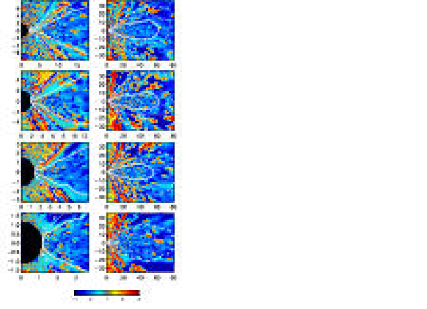
Figure 11: The azimuthally-averaged ratio $\langle b^{\phi}\,u^{r}\rangle/\langle b^{r}\,u^{\phi}\rangle$ , at $t=8080\,M$ in simulations with $a/M=0$ (first row from top), 0.5 (second row), 0.9 (third row), and 0.998 (fourth row). The left column shows the region inside $r=3\,r_{ms}$, the right column shows the main disk body; all are plotted on the same linear scale. Three azimuthally-averaged density contours are also shown, $\langle\rho\rangle$, scaled to the density maximum, $10^{-3}\,\rho_{max}$ (dashed line), $10^{-2}\,\rho_{max}$ (dotted line), $0.1\,\rho_{max}$ (solid line).

As illustrated in Figure 11, in general this ratio is quite different from unity. In most of the corona, disk body, inner torus, and plunging region it falls in the range $-0.3$ – $+0.3$, but there are locations near the funnel wall where the ratio spans a considerably wider range, with thin regions in the vicinity of the jet having values near unity. Values near unity are also found at the surface of the plunging flow above and below the main equatorial inflow, but even there the ratio fluctuates substantially in space and in time. We therefore conclude there is nothing to prevent significant electromagnetic energy fluxes in these accretion flows.

4.3 Dissipation Regions

These simulations were conducted with no explicit resistivity, and, consequently, they do not address where the magnetic field is dissipated or at what rate. However, regions of high current density are candidates for regions of high magnetic dissipation because high current density may trigger anomalous resistivity through mechanisms such as ion-acoustic turbulence (e.g., as suggested for the Solar corona by Rosner et al. 1978). We can locate these candidate dissipation regions by computing the current density from our simulation data. The current 4-vector is given by

$$J^{\mu}={1\over 4\,\pi}\,\nabla_{\mu}\,F^{\mu\nu},$$ (10)

where $\nabla_{\mu}$ is the covariant derivative and $F^{\mu\nu}$ the electromagnetic field-strength tensor. The covariant derivative simplifies to a simple derivative using the anti-symmetry of $F^{\mu\nu}$ (eq. 23 of DH03)

$$J^{\mu}={1\over 4\,\pi\,\sqrt{-g}}\,\partial_{\mu}\left(\alpha\,\sqrt{\gamma}\,g^{\mu\lambda}\,g^{\nu\xi}\,F_{\lambda\xi}\right),$$ (11)

where $F_{\lambda\xi}$ is directly related to the CT magnetic field and EMFs (eqs. 14 and 35 of DH03), the EMFs being simple functions of the CT magnetic field and transport velocities $V^{i}$. Evaluation of $J^{\mu}$ using code variables requires data for three adjacent time steps, since time derivatives must be evaluated. The current density then follows directly from these calculations, $\|J\|^{2}=J^{\mu}\,J_{\mu}$.

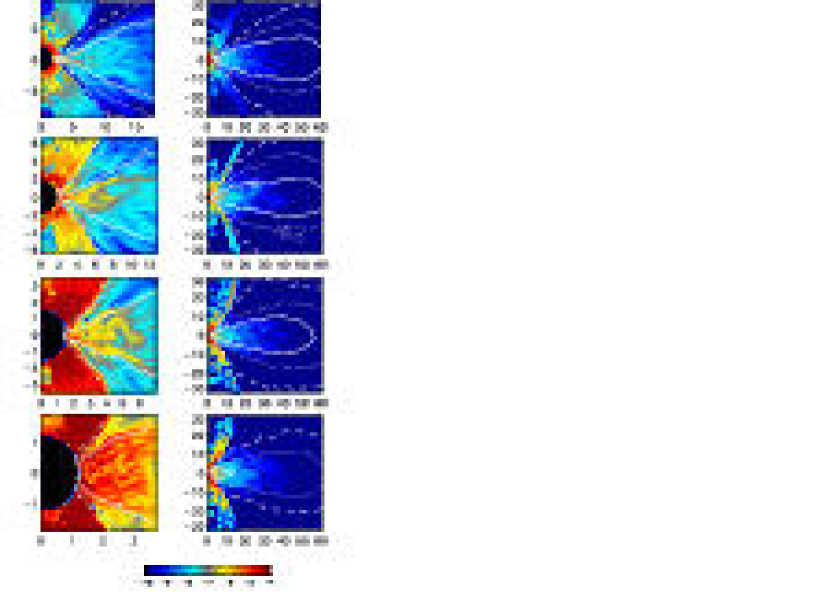
Figure 12: Azimuthally-averaged $\|J\|^{2}$ at $t=8080\,M$ in simulations with $a/M=0$ (first row from top), 0.5 (second row), 0.9 (third row), and 0.998 (fourth row). The left column shows the region inside $r=3\,r_{ms}$, the right column shows the main disk body; all are plotted on the same logarithmic scale. Three azimuthally-averaged density contours are also shown, $\langle\rho\rangle$, scaled to the density maximum, $10^{-3}\,\rho_{max}$ (dashed line), $10^{-2}\,\rho_{max}$ (dotted line), $0.1\,\rho_{max}$ (solid line).

Figure 12 shows azimuthally-averaged $\|J\|^{2}$ at a late time in each of the four simulations. The values are normalized to the initial torus total energy, $E_{0}$ ($\equiv\int\,d^{3}x^{i}\,\sqrt{-g}\,T^{t}_{t}$ in the initial state), to facilitate comparison between simulations. In all cases, regions of high current density in the accretion flow are found in extended sheets that run roughly parallel to density contours in the inner torus and plunging regions; currents in the main disk body are significantly weaker and less well organized, while the coronal envelope is quiescent. The axial funnel shows a current distribution similar to the distribution of magnetic pressure (Fig. 1). In all cases, the dynamic range between $\|J\|^{2}$ in one of the sheets and in the adjacent inner torus material is often two orders of magnitude. As with the magnetic pressure, there are also several systematic trends with black hole spin. The vertical thickness of the region in the disk body where high current density is found increases with $a/M$. The absolute level of $\|J\|^{2}$ (even after normalization to $E_{0}$) also increases with $a/M$, climbing by about a factor of 300 from $a/M=0$ to $a/M=0.998$.

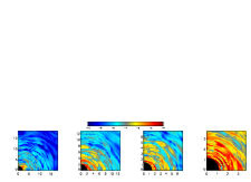
Figure 13: $\|J\|^{2}$ in the equatorial plane ($\theta=\pi/2$) at $t=8080\,M$ in simulations with (from left to right) $a/M=0$, 0.5, 0.9, and 0.998. In each case, the outermost radius shown is $3r_{ms}$. All are plotted on the same logarithmic scale as Figure 12.

Figure 13 shows $\|J\|^{2}/E_{0}$ in the equatorial plane ($\theta=\pi/2$) at a late time in each of the four simulations. This figure emphasizes the spiral structure of the currents. Here again, the steep radial gradient in current density can be seen. The regions of most intense current are almost all found within $\simeq 2r_{ms}$.

If we knew how to relate current density to dissipation rate, these maps would provide a basis for a map of heating in the accretion flow. In the absence of a physical model for the relation between current density and dissipation, we can instead give a qualitative sense for the heating distribution by integrating $\|J\|^{2}$ over volume in the disk, i.e., computing ${\cal J}\equiv\int\,d\theta d\phi\,\sqrt{-g}\,\|J\|^{2}$, but excluding those regions with $\rho<10^{-4}\rho_{\rm max}$, where $\rho_{\rm max}$ is the greatest density found anywhere in the simulation at that time. We ignore low-density regions in order to concentrate on possible heating in the accretion flow proper. The results are shown in Figure 14, again normalized to $E_{0}$. The left panel shows the integrated current density over the entire range of radii; the right panel shows the same quantity plotted as a function of $r/r_{ms}$. Both panels show the systematic increase in current density with black hole spin, particularly for $r<10M$. In the disk body, ${\cal J}$ declines steeply with increasing radius. Between $r_{ms}$ and $10r_{ms}$, $-2<d\ln{\cal J}/d\ln r<-1$, and the slope steepens at still larger radii. In the $a/M=0$ simulation, the integrated current density levels off slightly through the marginally stable orbit before rising sharply again near the inner boundary. For the other three simulations, the integrated current density has a sharp break upward near or inside $r_{ms}$, rising one to two orders of magnitude as the inner radial boundary is approached. Since frame dragging has been shown to increase magnetic pressure and azimuthal stretching of the field lines, this dramatic increase is not surprising. If the current density is indicative of the dissipation density, much of the total dissipation, especially around the most rapidly-spinning black holes, could occur very deep in the relativistic potential.

5 Discussion and Summary

In Paper I we divided the accretion flow into five distinct regions, each with its own characteristics, as follows: the main disk body, the inner torus and plunging region, the coronal envelope, the funnel, and the funnel wall jet. In this paper we have examined the magnetic field strengths and topologies in these regions.

5.1 Field Characteristics in the Different Flow Regions

The main disk body is characterized by MHD turbulence due to the MRI. As has been shown in previous studies, the magnetic field is very tightly wound by the differential rotation, but with significant poloidal tangling due to turbulence. The field wandering index shows that the poloidal field lines extend farther in the radial direction than in the polar. The field energies are subthermal, with plasma $\beta\approx 10$–100 on average. Strong fluctuations are the rule, however, and $\beta$ can exceed 1000 in some portions of the main disk body.

In the plunging region, the flow transitions from turbulence-dominated to spiraling inflow. A consequence of this is that the tight field winding loosens somewhat as the radial component of the velocity grows relative to the azimuthal component. This behavior is quantified approximately by the field-wandering and field-tangling indices, which show (see Figs. 8 and 9) that there is a sharp change of behavior near the marginally stable orbit. Field lines inside that radius travel farther in radius and much less in polar angle than in the disk body. This is a consequence of the transition from turbulent motions to more regular spiral inflow; that is, this break is yet another way of marking the turbulence edge defined by Krolik & Hawley (2002). Inside the plunging region the field is amplified relative to the fluid pressure. Near the horizon above and below the equator, $\beta$ falls from $\sim 10$ near $r_{ms}$ to less than 1. The equatorial flow itself maintains $\beta\sim 10$ or greater throughout the plunging region. These conclusions apply most clearly to the $a/M=0$, 0.5, and 0.9 simulations; the plunging region in the $a/M=0.998$ simulation is less well-resolved.

The field in the corona is, on average, in equipartition with the thermal energy there, and is dominated by the toroidal component; field line plots look smooth compared to those in the disk body. There are relatively extended poloidal fields, but these are more associated with outflowing toroidal coils. When field emerges from the disk body it carries some of the turbulent tangling with it, but this seems to be rapidly smoothed out. Gas is carried into the corona as well as magnetic field, so the corona does not become a magnetically dominated force-free region. The magnetic field does have a larger scale-height than the gas pressure, though.

By contrast, the field in the axial funnel is essentially radial outside the ergosphere, with a toroidal component that becomes larger with increasing black hole spin. In the funnel the magnetic field energy dominates over the matter energy, and the field can be regarded as force-free. The magnetic energy is not large compared to the magnetic energy in the remainder of the flow, however. The magnetic pressure in the funnel is in equilibrium with the total pressure in the corona and inner disk. From the field-connectivity data, we see that the magnetic field structure may be divided into two almost wholly independent regions: the accretion flow proper and the axial funnel. Field lines passing through the funnel almost never enter the other regions.

In the funnel-wall jet, the magnetic field configuration resembles that of the axial funnel, but the field lines are more tightly wound, consistent with the observation that the gas in the jet has specific angular momentum comparable to that at its injection point, above the inner torus. The jet is also less strongly magnetized than the axial funnel, with $\beta\simeq 0.3$.

The categorization of field line types listed in Table 1 and illustrated in Figure 5 provides a handy summary of the global field structure. It is important to recognize that only a subset of all possible field line types are found with any frequency in these simulations; the table indicates which these are. One of the most important global properties of the field is its inter-region connectivity. From this point of view, the different regions fall into two groups: the main disk body is linked to both the corona and the inner torus, while many field lines stretch from the inner torus to the plunging region. On the other hand, the field lines in the axial funnel have essentially no connection to the other regions.

5.2 Astrophysical Implications

The simulation results provide some insights into potentially important astrophysical processes that might occur in black hole accretion. For example, Livio et al. (1999) argued that energy extracted electromagnetically from the accretion disk proper would always outweigh that extracted from spinning black holes because the product of magnetic stress and area would be larger for the disks than for black hole event horizons. As Figure 1 shows, the total intensity of the magnetic field increases sharply inward. This is as true of the poloidal portion as the toroidal. Increases by factors $\sim 30$ from $r=5M$ to the plunging region are typical. Although it is true that, outside the funnel region, there is no large-scale poloidal field in this simulation, such large contrasts in field strength from disk to plunging region raise doubts about the Livio et al. hypothesis. Moreover, the force-free field in the evacuated funnel seems best configured to permit processes closely related to the Blandford-Znajek mechanism (Blandford & Znajek 1977), while the strength of the funnel field is comparable to that in the plunging region. These results suggest that accretion could well lead to a strong enough field near the event horizon that a genuine Blandford-Znajek process might yield more energy than competing processes associated more directly with the main disk body.

It is often asserted (in fact, frequently in connection with studies of the Blandford-Znajek mechanism) that the magnetospheres of black holes should be, in large part, effectively force-free (e.g., Okamoto 1992, Ghosh & Abramowicz 1997, Ghosh 2000, Park 2000, Blandford 2002, Komissarov 2002). In our simulations we find that the only region where the force-free approximation is applicable is the funnel. In the disk proper and most of the corona, the field structure is thoroughly matter-dominated; in the outer corona and parts of the plunging region, the energy density in the magnetic field begins to approach $\rho h$, but never exceeds it. Thus, the relativistic MHD approximation may be better-suited to work in this area than the relativistic electrodynamic approximation. It is possible, though, that cooling would alter the properties of the corona somewhat by significantly reducing the gas pressure scale height relative to that of the magnetic field.

A common suggestion for the origin of high-energy emission from accretion disks around black holes is that the footpoints of magnetic field lines in the corona are twisted in opposite directions by orbital shear, leading to reconnection (e.g., Blandford 2002). This process is initiated by establishment of a radial magnetic field link between two fluid elements arranged so that the outer one is advanced in orbital phase relative to the inner one. As the inner fluid element catches up to and passes the outer, an X-point would be formed. We see little evidence of this sort of process. What appears to happen instead is that when radial magnetic field links are created, it is between two fluid elements at nearly the same azimuthal angle (the closer two points are, the more likely they are to be magnetically connected). The orbital shear then creates a long azimuthal field line as the fluid element at the smaller radius moves ahead of the other fluid element. If the inner fluid element moves a full $2\pi$ in azimuth ahead of the outer one before reconnection occurs, the field lines wrap parallel to one another, rather than crossing near their footpoints.

It is generally believed that regions of high current density are likely to promote anomalous resistivity, and therefore be markers for regions of concentrated heat dissipation. Although we find that, if anything, current sheets are especially rare in the corona, they are very common and very intense in the innermost parts of the accretion flow, particularly the plunging region. The possibility of substantial heat release inside $r_{ms}$ has an interesting consequence. In the Novikov-Thorne theory of relativistic accretion disks, the energy made available for radiation is the difference between the potential energy lost by accreting matter and the work done by accretion stresses. Because they assumed that all stresses vanish inside $r_{ms}$, there is no energy released inside that radius. If the Novikov-Thorne model is generalized to allow non-zero stress at $r_{ms}$ (e.g., Agol & Krolik 2000), the amount of energy dissipated inside the disk rises, but it is still determined in essentially the same way. Dissipation inside $r_{ms}$ is an entirely new and independent mechanism of energy release. It is not necessarily associated with angular momentum transport; it could result from entirely local processes (e.g., Machida & Matsumoto 2003). Nonetheless, if the time to radiate this heat is shorter than an infall time, the photons released could carry off the energy to infinity, adding to the light seen by distant observers.

One of the main purposes of carrying out these simulations across a broad range of black hole spins is to extract information previously unobtainable from pseudo-Newtonian simulations of accreting tori. The spacetime rotation caused by spinning black holes is a notable example of this sort of effect. Perhaps the most striking spin-dependent property of the magnetic fields is the increase in magnetic pressure near the black hole with increasing spin. This pressure increase is found at the surface of the inner torus and plunging region (i.e., off the equatorial plane), as well as deep in the axial funnel. There is also a corresponding increase in gas pressure in this region, so that the ratio of pressures ($\beta$) remains effectively unchanged. The growth of magnetic pressure is due in part to the dragging of field lines by the black hole, and in part to the inward displacement of the marginally stable orbit with black hole spin, which tends to allow the MRI to operate closer to the event horizon. There is also a strong spin-dependent growth in the intensity of currents in the vicinity of the black hole. In the $a/M=0$, 0.5, and 0.9 simulations, the high current regions are organized in sheets through the inner torus; these current sheets also have a spiral character, inherited from gas motion in the vicinity of the plunging region. The $a/M=0.998$ simulation shows a much more intense and turbulent current distribution, reflecting the fact that the plunging region is extremely narrow in Boyer-Lindquist coordinates and the the inner torus extends deep into the ergosphere. This strong spin-dependence of the currents suggests that magnetic dissipation may be especially intense in accretion flows near extreme black holes.

Table 1: Field Line Varieties (after Blandford 2002)

Type Number	Description	Common?
1	tangled within the disk body	yes
2	loops linking regions of disk through corona	no
3	poloidal from disk to infinity	no
4	linking accreting matter in plunging region to disk body	yes
5	linking high latitudes on event horizon to disk body	no
6	poloidal from event horizon to infinity	yes
7	poloidal from matter in plunging region to infinity	no
8	smooth tightly-wrapped coronal spiral	yes
9	poloidal field linking horizon to accretion flow	yes

Figure 8: Wandering index (see text for definition) as a function of radial coordinate of the field line’s starting point for each of the four black hole spins considered. The curves are: $a/M=0$ simulation (solid line); $a/M=0.5$ simulation (dotted line); $a/M=0.9$ simulation (dashed line); and $a/M=0.998$ simulation (dash-dot line). Left-hand panel: Radial wandering. Right-hand panel: Polar angle wandering.

Figure 9: The field-tangling index $\Psi$ as a function of $r_{o}$ inside the disk body ($0.45\pi<\theta<0.55\pi$: left panel) and $\theta_{o}$ ($10M<r<15M$: right panel). The curves are: $a/M=0$ simulation (solid line); $a/M=0.5$ simulation (dotted line); $a/M=0.9$ simulation (dashed line); and $a/M=0.998$ simulation (dash-dot line).

Figure 10: The cumulative distribution of tangling $\Psi(<\sigma)=\int_{0}^{\sigma}\,d\sigma^{\prime}\sigma^{\prime}dN/d\sigma^{\prime}$ averaged over ten late-time snapshots in the $a/M=0.9$ simulation at the radii shown and within $0.05\pi$ radians of the equatorial plane. Here $dN/d\sigma$ is the number distribution of bend angles.

Figure 14: Shell-integrated current density, (see text for definition) plotted as a function of $r/M$ (left panel) and $r/r_{ms}$ (right panel) for the $a/M=0$ simulation (solid line), 0.5 simulation (dotted line), 0.9 simulation (dashed line), and 0.998 simulation (dash-dot line). The integral over $\theta$ includes only that region where $\rho>10^{-4}\,\rho_{max}$, thereby excluding the funnel.

References

- Agol & Krolik (2000) Agol, E. & Krolik, J. H. 2000, ApJ 528, 161
- Armitage et al. (2001) Armitage, P.J., Reynolds, C.S. & Chiang, J. 2001, ApJ 548, 868
- Armitage & Reynolds (2003) Armitage, P.J. & Reynolds, C.S. 2003, MNRAS 341, 1041
- Balbus & Hawley (1998) Balbus, S. A., & Hawley, J. F. 1998, Rev. Mod. Phys., 70, 1
- Bisnovatyi-Kogan & Ruzmaikin (1976) Bisnovatyi-Kogan, G. & Ruzmaikin, A. 1976, Ap. Sp. Sci. 42, 401
- Blandford (2002) Blandford, R.D. 2002, in Lighthouses of the Universe: The Most Luminous Celestial Objects and Their Use for Cosmology: Proceedings of the MPA/ESO/Workshop, eds. M. Gilfanov, R. Sunyaev, E. Churazov (New York: Springer), 381
- Blandford & Znajek (1977) Blandford, R.D. & Znajek, R.L. 1977, MNRAS 179, 433
- De Villiers, & Hawley (2003) De Villiers, J. P. & Hawley, J. F. 2003, ApJ, 589, 458 (DH03)
- De Villiers et al. (2003) De Villiers, J. P., Hawley, J. F. & Krolik, J. H. 2003, ApJ, 599, in press (Paper I)
- Gammie (1999) Gammie, C.F. 1999, ApJLetts 522, 57
- Ghosh (2000) Ghosh, P. 2000, MNRAS 315, 89
- Ghosh & Abramowicz (1997) Ghosh, P. & Abramowicz, M. 1997, MNRAS 292, 887
- Hawley (2000) Hawley, J. F. 2000, ApJ, 528, 462
- Hawley & Krolik (2001) Hawley, J. F. & Krolik, J. H. 2001, ApJ, 548, 348
- Hawley & Krolik (2002) Hawley, J. F. & Krolik, J. H. 2002, ApJ, 566, 164
- Komissarov (2002) Komissarov, S.S. 2002, MNRAS 336, 759
- Krolik (1999) Krolik, J. H. 1999, ApJL, 515, 73
- Krolik & Hawley (2002) Krolik, J. H. & Hawley, J. F. 2002, ApJ 573, 754
- (19) Li, L.-X. 2003a, Phys Rev D, 67, 4007
- (20) Li, L.-X. 2003b, Phys Rev D, 68, 24022
- Livio et al. (1999) Livio, M., Ogilvie, G.I. & Pringle, J.E. 1999, ApJLetts 512, L100
- Lubow et al. (1994) Lubow, S.H., Papaloizou, J. & Pringle, J.E. 1994, MNRAS 268, 1010
- Machida & Matsumoto (2003) Machida, M. & Matsumoto, R. 2003, ApJ 585, 429
- Miller & Stone (2000) Miller, K. A., & Stone, J. M. 2000, ApJ, 534, 398
- Misner, Thorne, & Wheeler (1973) Misner, C. W., Thorne, K. S., & Wheeler, J. A 1973, Gravitation (San Francisco: W.H. Freeman)
- Novikov & Thorne (1973) Novikov, I.D. & Thorne, K.S. 1973, in Black Holes: Les Astres Occlus, eds. C. de Witt & B. de Witt (New York: Gordon & Breach), 344
- Okamoto (1992) Okamoto, I. 1992, MNRAS 254, 192
- Park (2000) Park, S.-J. 2000, JKAS 33, 19
- Rosner et al. (1978) Rosner, R., Golub, L., Coppi, B. & Vaiana, G.S. 1978, ApJ 222, 317
- (30) Thorne, K.S., Price, R.H. & MacDonald, D.A. 1986, Black holes: The Membrane Paradigm (New Haven: Yale University Press)