Adiabatic relativistic models for the jets in the radio galaxy 3C 31

Abstract

We present a general approach to the modelling of the brightness and polarization structures of adiabatic, decelerating relativistic jets, based on the formalism of Matthews & Scheuer (1990). We compare the predictions of adiabatic jet models with deep, high-resolution observations of the radio jets in the FR I radio galaxy 3C 31. Adiabatic models require coupling between the variations of velocity, magnetic field and particle density. They are therefore more tightly constrained than the models previously presented for 3C 31 by Laing & Bridle (2002a). We show that adiabatic models provide a poorer description of the data in two crucial respects: they cannot reproduce the observed magnetic-field structures in detail, and they also predict too steep a brightness decline along the jets for plausible variations of the jet velocity. We find that the innermost regions of the jets show the strongest evidence for non-adiabatic behaviour, and that the adiabatic models provide progressively better descriptions of the jet emission at larger distances from the galactic nucleus. We briefly discuss physical processes which might contribute to this non-adiabatic behaviour. In particular, we develop a parameterized description of distributed particle injection, which we fit to the observed total intensities. We show that particles are preferentially injected where bright X-ray emission is observed, and where we infer that the jets are over-pressured.

1 Introduction

This paper is one of a series whose aim is to develop quantitative models of jets in low-luminosity (FR I; Fanaroff & Riley 1974) radio galaxies on the assumption that they are decelerating relativistic flows. Our hypothesis is that the jets are close enough to being intrinsically symmetrical, axisymmetric and antiparallel that the observed differences between them are dominated by the effects of relativistic aberration. This hypothesis is motivated by the results of Laing et al. (1999), who presented a statistical study of jets in the B2 sample of radio galaxies and showed that the observed correlations between fractional core flux density and side-to-side asymmetries in intensity and width are consistent with jet deceleration and the presence of transverse velocity gradients. They inferred that the jets slow from $\approx$0.9$c$ where they start to expand rapidly to $\approx$0.1$c$ over distances $\sim$1 to 10 kpc and that the deceleration scale is an increasing function of jet power. In Laing & Bridle (2002a, hereafter LB), we demonstrated that an intrinsically symmetrical, relativistic jet model provides an excellent description of the total intensity and linear polarization observed at 8.4 GHz from the jets of the FR I radio galaxy 3C 31. We were able to estimate the angle to the line of sight and the three-dimensional distributions of velocity, emissivity and magnetic-field structure. By combining this kinematic model with a description of the external gas density and pressure derived from Chandra observations (Hardcastle et al., 2002) and using conservation of particles, energy and momentum, we demonstrated that the jet deceleration could be produced by entrainment of thermal matter and we derived the spatial variations of pressure, density and entrainment rate (Laing & Bridle, 2002b).

The free models developed by LB for 3C 31 were designed to fit the observed images without embodying specific preconceptions about the (poorly known) internal physics. In those models, we adopted simple and arbitrary functional forms for the spatial variations of velocity, synchrotron emissivity and field ordering and allowed the emissivity and field ordering to vary separately as smooth functions of position. To proceed beyond such purely empirical descriptions of the jets, we must make further assumptions about processes that affect the components of the modelled emissivity – the relativistic particle energy spectrum and the strength of the magnetic field. The separation of the emissivity into its components is ill-determined unless inverse-Compton emission can be detected from the synchrotron-emitting electrons, in which case the particle density and field strength can be determined independently. Unfortunately, inverse-Compton emission from the inner jets in 3C 31 is too weak to detect (Hardcastle et al., 2002). There are, as yet, no prescriptive theories for dissipative processes such as particle acceleration and field amplification or reconnection in conditions appropriate to FR I radio jets.

The energy-loss processes for the radiating particles can be quantified, however. It is inevitable that the particles will suffer adiabatic losses as the jets expand. We argue that synchrotron and inverse-Compton losses are negligible by comparison for electrons radiating at 8.4 GHz in 3C 31, as the jets have accurately power-law spectra with indices close to 0.5 (Laing et al., 2004) and show no evidence of spectral curvature until much higher frequencies (Hardcastle et al., 2002). It is therefore worthwhile to compare the observations with models in which the radiating particles are accelerated before entering the region of interest and then lose energy only by the adiabatic mechanism while the magnetic field is frozen into and convected passively with the flow, which is assumed to be laminar. Following conventional usage, we refer to such models as adiabatic.

There are analytical solutions for the adiabatic evolution of emissivity and surface brightness with jet radius and velocity if the magnetic field is exactly parallel or perpendicular to the flow direction. Models of this kind were first considered by Burch (1979), who showed that the decrease of brightness with distance from the nucleus would be much steeper than he observed in 3C 31 if the jets have constant velocity. Fanti et al. (1982) pointed out that the brightness would decline more slowly with distance in a decelerating jet. This idea underlies the turbulent jet models of Bicknell (1984, 1986). A relativistic generalisation was developed by Baum et al. (1997) to model the jets in 3C 264 and was applied by Feretti et al. (1999) and Bondi et al. (2000) to other FR I jets. These treatments all assumed that there is no velocity gradient across the jet, and that the magnetic field is exactly parallel or perpendicular to the flow. While this approach is self-consistent, it cannot be applied if there is velocity shear in a direction perpendicular to any component of the field.

In LB, we developed a numerical approach to modelling a relativistic jet with a more general magnetic field structure. This approach allowed us to use the variations of total intensity and linear polarization as independent constraints on the jet velocity field. We concluded that the magnetic structure and velocity field in 3C 31 are indeed significantly more complex than those assumed by Baum et al. (1997). Nevertheless, we compared our models and the data for 3C 31 with their analytical solutions. We showed that:

1. the adiabatic approximation is qualitatively inconsistent with the variations of brightness and polarization along the first $\approx$3 kpc of the jets, but

2. further from the nucleus, the observed variations are closer to those expected if the adiabatic approximation holds.

This comparison motivated us to develop a more general approach to modelling of adiabatic, relativistic jets, which we present in this paper. Our approach allows us to calculate how the brightness and polarization structure evolve along an adiabatic jet from prescribed initial conditions (specified as profiles across the jet), given the jet geometry and more complex magnetic structures and velocity fields of the type inferred for 3C 31 by LB. Detailed comparison of the new adiabatic models with the free models of LB, which fit the observations better, can then diagnose whether and where other physical processes, such as particle acceleration, may be significant in the jets.

Section 2 reviews our assumptions and the previous analytical solutions, and then outlines our calculation of synchrotron emission from adiabatic flows. Section 3 describes our approach to modelling of adiabatic jets; it briefly recapitulates material from LB before discussing new aspects specific to the present study. Section 4 applies our adiabatic models to the outer regions of the jets in 3C 31 and shows that they can give a fair description of the VLA observations of these regions. Section 5 confirms that the adiabatic models fail to describe the inner jet regions and critiques the adiabatic hypothesis in the light of this result; it also discusses the extent to which distributed particle injection can bring the adiabatic models into better agreement with the data. Section 6 summarizes our conclusions.

2 The adiabatic approximation

2.1 Assumptions

The jets are taken to be adiabatic in the sense defined by Burch (1979), Matthews & Scheuer (1990) and Baum et al. (1997), as follows:

1. The energies of the radiating particles change like those in an adiabatically expanding relativistic gas, i.e. $\propto V^{-1/3}$, where $V$ is the volume of a fluid element in its rest frame.

2. There is no diffusion of particles.

3. The particle momentum distribution remains isotropic (e.g. by resonant scattering off Alfvén waves).

4. The magnetic field behaves as if it is convected passively with the flow. We take the velocity field to be a smooth function of position. Although the addition of a turbulent velocity component would make little difference to the calculation of the effects of relativistic aberration on the appearance of the jet, there would be a major difference in the strength and structure of the magnetic field, which would be affected by shear and expansion, if not by dynamo action and reconnection.

5. Synchrotron and inverse-Compton losses are negligible for electrons radiating at the wavelength of observation, so the energy and synchrotron frequency spectra are always power laws with indices $-(2\alpha+1)$ and $-\alpha$, respectively. Specifically, we take the number density of radiating electrons with energies between $E$ and $E+dE$ in the jet rest frame to be

   $$N(E)dE=nE^{-(2\alpha+1)}dE$$ (1)

In addition, we assume, as in LB, that the regions of the jets to be modelled are intrinsically identical, antiparallel, axisymmetric, stationary flows.

The magnetic field $B$ is taken to have longitudinal, toroidal and radial components $B_{l}$, $B_{t}$ and $B_{r}$ (all measured in the jet rest frame). Synchrotron radiation is generally anisotropic even in the rest frame of the emitting material. In this paper we therefore write the emissivity $\epsilon({\bf r})g({\bf r})$, where $\epsilon({\bf r})$ would be the emissivity in total intensity for a magnetic field $\langle B_{l}^{2}+B_{t}^{2}+B_{r}^{2}\rangle^{1/2}$ perpendicular to the line of sight ($\langle\rangle$ denotes a spatial average). $\epsilon({\bf r})$ is the same for all three Stokes parameters, but $g({\bf r})$ depends on field geometry, and differs for $I$, $Q$ and $U$ [for total intensity, $0\leq g_{I}({\bf r})\leq 1$ and for linear polarization $-p_{0}\leq g_{Q,U}({\bf r})\leq p_{0}$, where $p_{0}=(3\alpha+3)/(3\alpha+5)$ is the maximum degree of polarization for spectral index $\alpha$].

2.2 Analytical approximations

We now briefly recapitulate the analytical adiabatic relations derived by Baum et al. (1997) for axisymmetric, decelerating, relativistic jets without velocity shear. Suppose that a jet has radius $R$, and that we can make the quasi-one-dimensional approximation: (a) that it is uniform in cross-section at a given distance from the nucleus and (b) that the velocity is unidirectional. The field components and the normalizing constant in the energy spectrum, $n$, vary as:

$$B_{l} \propto R^{-2}$$ (2)

$$B_{t} \propto (R\beta\Gamma)^{-1}$$ (3)

$$B_{r} \propto (R\beta\Gamma)^{-1}$$ (4)

$$n \propto (\Gamma\beta R^{2})^{-(1+2\alpha/3)}$$ (5)

where the velocity of the jet is $\beta c$ and $\Gamma=(1-\beta^{2})^{-1/2}$.

For a purely longitudinal field ($B_{t}=B_{r}=0$), this leads to a variation of the rest-frame emissivity:

$$\epsilon \propto (\Gamma\beta)^{-(2\alpha+3)/3}R^{-(10\alpha+12)/3}$$ (6)

and for a perpendicular field ($B_{l}=0$):

$$\epsilon \propto (\Gamma\beta)^{-(5\alpha+6)/3}R^{-(7\alpha+9)/3}$$ (7)

For conical jets, the radius is proportional to distance from the nucleus, $r$, so identical relations are obtained with $r$ replacing $R$.

In the absence of velocity shear, the adiabatic relations for the magnetic field can be combined to describe arbitrary initial conditions. The total field $B$ is then:

$$B=\left[\bar{B}_{l}^{2}\left(\frac{\bar{R}}{R}\right)^{4}+(\bar{B}_{t}^{2}+\bar{B}_{r}^{2})\left(\frac{\bar{\Gamma}\bar{\beta}\bar{R}}{\Gamma\beta R}\right)^{2}\right]^{1/2}$$ (8)

where $\bar{B}_{l}$, $\bar{B}_{t}$ and $\bar{B}_{r}$ are the initial field components, $\bar{\beta}$ and $\bar{\Gamma}$ are the velocity and Lorentz factor, all defined where the jet radius is $R=\bar{R}$. The emissivity is then:

$$\epsilon\propto(\Gamma\beta R^{2})^{-(1+2\alpha/3)}B^{1+\alpha}$$ (9)

The next subsection develops a numerical approach capable of describing velocity shear.

2.3 Adiabatic flows with arbitrary initial conditions and velocity fields

The formalism needed to predict the total and linearly polarized synchrotron emission from an element of fluid in a non-relativistic adiabatic flow was first developed by Matthews & Scheuer (1990). Their approach was to follow an element of fluid containing relativistic particles and an initially isotropic, disordered magnetic field through a model flow. They included the effects of synchrotron and inverse-Compton energy losses, as well as adiabatic effects. Laing (2002) developed a simplified approach for the case where synchrotron and inverse-Compton losses are negligible, which we follow here. The reasons for taking the field to be disordered on small scales are discussed by Laing (1981), Begelman, Blandford & Rees (1984) and LB.

An element of fluid is taken to be a unit cube (much smaller than the spatial scale of variations in the velocity field), with sides defined by orthonormal unit vectors ${\bf\hat{a}}$, ${\bf\hat{b}}$ and ${\bf\hat{c}}$ along natural axes of the flow in the fluid rest frame. The cube contains an isotropic disordered field and relativistic particles with the energy spectrum of equation (1) and normalizing constant $\bar{n}$. The cube moves with the flow, deforming into a parallelepiped with sides defined by the vectors ${\bf a}$, ${\bf b}$ and ${\bf c}$. Application of flux conservation shows that an element of field which is initially ${\bf\bar{B}}=\bar{B}_{x}{\bf\hat{a}}+\bar{B}_{y}{\bf\hat{b}}+\bar{B}_{z}{\bf\hat{c}}$ becomes:

$${\bf B}=\frac{\bar{B}_{x}{\bf a}+\bar{B}_{y}{\bf b}+\bar{B}_{z}{\bf c}}{V}$$ (10)

where $V={\bf a\cdot b\times c}$ is the volume of the parallelepiped evaluated in the fluid rest frame. The energy spectrum constant $n$ evolves according to:

$$n=\bar{n}V^{-(1+2\alpha/3)}$$ (11)

We assume that the flow is axisymmetric, with deceleration and a transverse velocity gradient. We define a second coordinate system $(x,y,z)$, again in the observed frame, with $z$ along the jet axis, $x$ perpendicular to it in a plane containing the line of sight and $y$ in the plane of the sky. We parameterize the streamline by an index $s$, which varies from 0 at the inner edge of a flow component to 1 at its outer edge, as in LB. Without loss of generality, we can consider flow in the $x,z$ plane, where the distance of a streamline from the jet axis is $x(z,s)$.

The geometry and evolution of the vectors ${\bf a}$, ${\bf b}$ and ${\bf c}$ are sketched in Fig. 1. As an element of fluid moves outwards, ${\bf c}$ remains parallel to the streamline and its magnitude is determined entirely by the flow velocity. ${\bf b}$ is unaffected by shear and is orthogonal to the flow direction, so its magnitude is proportional to the distance of the streamline from the jet axis. ${\bf a}$ (initially radial) is the only one of the three vectors affected by velocity shear: it is a function of the jet radius and the accumulated path length difference along adjacent streamlines (Fig. 1). Four quantities are therefore needed to describe the shape of the parallelepiped: three expansion factors and a shear term. For a streamline in the $xz$ plane, the vectors are:

$${\bf a} = \frac{\partial x/\partial s}{\partial\bar{x}/\partial s}\left(\frac{1+\bar{x}^{\prime 2}}{1+x^{\prime 2}}\right)^{1/2}{\bf l}+\frac{\Gamma}{\bar{\Gamma}}f{\bf n}$$ (12)

$${\bf b} = \frac{x}{\bar{x}}{\bf m}$$ (13)

$${\bf c} = \frac{\Gamma\beta}{\bar{\Gamma}\bar{\beta}}{\bf n}$$ (14)

and the volume is

$$V={\bf a\cdot b\times c}=\frac{\Gamma\beta}{\bar{\Gamma}\bar{\beta}}\frac{x}{\bar{x}}\frac{\partial x/\partial s}{\partial\bar{x}/\partial s}\left(\frac{1+\bar{x}^{\prime 2}}{1+x^{\prime 2}}\right)^{1/2}$$ (15)

${\bf l}$, ${\bf m}$ and ${\bf n}$ are (orthonormal) unit vectors along the local radial, toroidal and longitudinal directions, respectively and primes denote differentiation with respect to $z$ for a given streamline. Barred quantities are evaluated at the starting surface. The factor of $\Gamma/\bar{\Gamma}$ in equations 12 and 14 accounts for Lorentz contraction along the flow direction.

$f$ is the shear term, which does not affect the volume. It will usually be $<0$ if the velocity decreases outwards from the jet axis. We evaluate it by considering two elements of fluid which leave the reference surface at time $t=0$ on adjacent streamlines with indices $s$ and $s+\Delta s$. After a time $t$, we have

$$ct = \int\frac{dl}{\beta}$$

$$= \int^{z(s)}_{\bar{z}(s)}\frac{[1+x^{\prime}(z,s)^{2}]^{1/2}dz}{\beta(z,s)}$$

$$= \int^{z(s+\Delta s)}_{\bar{z}(s+\Delta s)}\frac{[1+x^{\prime}(z,s+\Delta s)^{2}]^{1/2}dz}{\beta(z,s+\Delta s)}$$

where $dl$ is an element of path along the streamline and $\bar{z}(s)$ and $z(s)$ are the $z$-coordinates of the fluid element at the reference surface and after time $t$, respectively, We express the integral for streamline $s+\Delta s$ as the sum of the integral for streamline $s$ and a set of terms expanded to first order in $\Delta s$ and $\Delta z=z(s+\Delta s)-z(s)$. The reference surface is spherical, and is always set in a part of the jet where the streamlines are straight, so a streamline crosses the surface at $z=\bar{z}$ with

$$x(\bar{z},s)=\bar{r}\cos[\bar{\zeta}+(\bar{\xi}-\bar{\zeta})s]$$ (17)

(see Section 3.2). This allows us to evaluate $\Delta z/\Delta s$ using the relation

$$\frac{\Delta z}{\Delta s}\left[\frac{1+x^{\prime 2}}{\beta}\right] = -\frac{(\bar{\xi}-\bar{\zeta})\bar{r}\tan[\bar{\zeta}+(\bar{\xi}-\bar{\zeta})s]}{\bar{\beta}}$$

$$- \int^{z}_{\bar{z}}\frac{\beta x^{\prime}\partial x^{\prime}/\partial s-(1+x^{\prime 2})\partial\beta/\partial s}{\beta^{2}(1+x^{\prime 2})^{1/2}}dz$$

The difference in path length along the streamline, $\Delta l$, is given by

$$\frac{\Delta l}{\Delta s}=(1+x^{\prime 2})^{1/2}\left[\frac{\Delta z}{\Delta s}+\frac{\partial x}{\partial s}\frac{x^{\prime}}{1+x^{\prime 2}}\right]$$ (19)

Finally, the shear term $f$ is the component of ${\bf a}$ along the streamline normalized by the magnitude of the vectors at the reference surface:

$$f=\frac{1}{\bar{r}(\bar{\xi}-\bar{\zeta})}\frac{\Delta l}{\Delta s}$$ (20)

$f$ is negative if the velocity decreases with increasing $s$.

In general, calculation of the shear term requires a numerical integration, but for regions of the jet where the streamlines are straight and the variation of the velocity along a streamline is a simple function, it can be done analytically. Note also that the shear term is non-zero even for a velocity independent of $s$ if the streamlines are curved.

For flow radially outwards from the nucleus, the three vectors and the volume element can be written very simply in terms of the distance from the nucleus, $r=(x^{2}+y^{2}+z^{2})^{1/2}$:

$${\bf a} = \frac{r}{\bar{r}}{\bf\hat{a}}+\frac{\Gamma}{\bar{\Gamma}}f{\bf\hat{c}}$$ (21)

$${\bf b} = \frac{r}{\bar{r}}{\bf\hat{b}}$$ (22)

$${\bf c} = \frac{\Gamma\beta}{\bar{\Gamma}\bar{\beta}}{\bf\hat{c}}$$ (23)

$$V = \frac{\Gamma\beta r^{2}}{\bar{\Gamma}\bar{\beta}\bar{r}^{2}}$$ (24)

In the absence of shear ($f=0$) these are equivalent to the relations derived by Baum et al. (1997) and given in equations 2–5.

Figure 1: Sketches of the evolution of the vectors ${\bf a}$, ${\bf b}$ and ${\bf c}$ defined in the text (not to scale). Panel (a) shows two neighbouring streamlines with indices $s$ and $s+\Delta s$ (defined in Section 2.3), in a plane containing the jet axis in a part of the jet where the flow direction changes with distance from the nucleus. ${\bf\hat{b}}$ and ${\bf b}$ are perpendicular to the plane of the diagram, and are not shown. Note that ${\bf c}$ remains parallel to the flow despite the change in direction. Panel (b) shows a projection of the flow in three dimensions viewed with the jet axis at 45^∘ to the line of sight in a region where the streamlines are straight. The full line is a representative streamline. The ellipses represent the positions of fluid elements with streamline indices $s$ and $s+\Delta s$. The lower pair are at the surface where the initial conditions are set and the upper pair represent the positions reached by the fluid elements after a given time. The vector ${\bf a^{\prime}}$, shown dashed, is the value of ${\bf a}$ in the absence of shear.

Laing (2002) gives the variation of the field components perpendicular to the line of sight in terms of the direction cosines of the vectors ${\bf a}$, ${\bf b}$ and ${\bf c}$ with respect to a fixed coordinate system $(X,Y,Z)$ with $Z$ along the line of sight. Together with $n$, these determine the synchrotron emissivity in Stokes $I$, $Q$ and $U$.

There are two additional complications:

1. The direction cosines must be evaluated in the rest frame of the fluid (exactly as for the free models of LB).

2. We need to set initial conditions on a reference surface in the jet, rather than starting with an isotropic magnetic field. We do this by adjusting the relative magnitudes of the vectors ${\bf\hat{a}}$, ${\bf\hat{b}}$ and ${\bf\hat{c}}$ in such a way as to produce the desired ratios between the three field components whilst leaving the volume (and therefore the rms total field and the emissivity function, $\epsilon$) unchanged.

3 Observations and modelling methods

3.1 Observations

The deep, high-resolution VLA observations with which we compare our models are described in LB. We take the Hubble constant to be $H_{0}$ = 70 km s^-1 Mpc^-1. At the redshift of 3C 31 (0.0169; Smith et al. 2000, Huchra, Vogeley & Geller 1999, De Vaucouleurs et al. 1991), the linear scale is then 0.34 kpc/arcsec. We fit our models to images at resolutions of 0.75 and 0.25 arcsec, covering the inner $\pm$28 arcsec of the jets. Fig. 2 shows the emission from the jets of 3C 31 with the area we model outlined.

Figure 2: A grey-scale of the total intensity from the jets of 3C 31 at 8.4 GHz (LB). The resolution is 0.25 arcsec FWHM and the area we model is indicated by the box.

3.2 Geometry

In LB, we showed that the jets in 3C 31 could be divided into three regions according to the shapes of their outer isophotes. As observed (i.e. projected on the plane of the sky), these are:

1. Inner (0 – 2.5 arcsec): a cone, centred on the nucleus, with a projected half-opening angle of 8.5 degrees.

2. Flaring (2.5 – 8.3 arcsec): a region in which the jet initially expands much more rapidly and then recollimates.

3. Outer (8.3 – 28.3 arcsec): a second region of conical expansion, also centred on the nucleus, but with a projected half-opening angle of 16.75 degrees.

We showed that these regions also have distinct kinematic properties.

We use the same descriptions of jet geometry and velocity as in LB, where we investigated two different transverse velocity structures. In the first (spine/shear layer – SSL) a central fast spine with no transverse variation of velocity is surrounded by a slower shear layer with a linear velocity gradient. In the second (Gaussian), there is no distinct spine component, and the jet consists entirely of a shear layer with a truncated Gaussian velocity law. The streamline index, $s$ (defined in table 3 of LB) varies from 0 for the streamline closest to the axis in the spine or shear layer to 1 for the furthest streamline. The angles $\bar{\zeta}$ and $\bar{\xi}$ used in Section 2.3 are the opening angles of the spine and shear layer, respectively, at the reference surface for an adiabatic model.

Table 1: The functional variation of velocity along the model jets.

Quantity	Free parameters				Functional dependences
	$r_{1}$	$r_{0}$	$r_{\rm f}$	Other	Flaring	Outer
	On-axis velocities
$\beta_{\rho}(\rho)$	$\beta_{1}$	$\beta_{0}$	$\beta_{\rm f}$	$H$	$b_{0}+b_{1}\rho^{H-1}+b_{2}\rho^{H}$	$c_{0}\exp(-c_{1}\rho)$
	Fractional edge velocities
$\bar{v}(\rho)$	$v_{1}$	$v_{0}$			$v_{1}+\frac{(\rho-r_{1})(v_{0}-v_{1})}{r_{0}-r_{1}}$	$v_{0}$

The angle between the jet axis and the line of sight is taken to be $\theta$ and we use the $xyz$ coordinate system defined earlier. In the inner and outer regions the streamlines are straight. In the flaring region we interpolate using a cubic polynomial in such a way that $x(z,s)$ and its first spatial derivative $x^{\prime}(z,s)$ are continuous at the boundaries between regions, which are spherical, centred on the nucleus with radii $r_{1}$ and $r_{0}$. The assumed geometry is sketched in Fig. 3.

Figure 3: Geometry of the spine/shear-layer model, showing the inner, flaring and outer regions in the plane containing the jet axis. The thick full curves represent the edge of the jet, the boundaries between regions are represented by thin full curves and the $s=0.5$ streamlines for the spine and shear layer are drawn as dashed curves. (a) The entire modelled region; (b) the base of the jet on a larger scale, showing the boundary surfaces at distances of $r_{1}$ and $r_{0}$ from the nucleus. The Gaussian model is essentially the same, but with the spine component removed.

In order to describe velocity variations along a streamline, we use a coordinate $\rho$, defined as:

$$\rho = r\makebox{~{}~{}(inner region)}$$

$$\rho = r_{1}+(r_{0}-r_{1})\frac{z-r_{1}\cos\phi_{\rm i}(s)}{r_{0}\cos\phi_{\rm o}(s)-r_{1}\cos\phi_{\rm i}(s)}$$

     (flaring region)

$$\rho = r\makebox{~{}~{}(outer region)}$$

where the streamline makes angles $\phi_{\rm i}$ and $\phi_{\rm o}$ with the axis in the inner and outer regions, respectively. $\rho$ is monotonic along any streamline and varies smoothly from $r_{1}$ to $r_{0}$ through the flaring region. This allows us to match on to simple velocity profiles which depend only on $r$ in the inner and outer regions.

The functions defining the edge of the jet are constrained to match the observed outer isophotes and are fixed in a coordinate system projected on the sky. Their values in the jet coordinate system then depend only on the angle to the line of sight.

3.3 Velocity field

The velocity field is taken to be a separable function $\beta(\rho,s)=\beta_{\rho}(\rho)\beta_{s}(s)$ with $\beta_{s}(0)=1$. The variation along a streamline, $\beta_{\rho}(\rho)$ is given in Table 1, and is exactly as in LB, omitting the inner region, which we do not discuss quantitatively in this paper. It is defined by the index $H$, together with velocities at three locations in the jet: $r_{1}$, $r_{0}$ and an arbitrary fiducial distance $r_{f}$. These distances are fixed by their projections on the plane of the sky, which are 2.5 arcsec, 8.2 arcsec and 22.4 arcsec, respectively. The form of $\beta_{\rho}(\rho)$ was chosen by LB (Section 3.4) to permit fitting the sidedness-ratio profile observed in 3C 31, which requires the velocity to remain constant through most of the flaring region but then to drop abruptly close to the outer boundary, at a rate determined by the index $H$. The velocity then falls smoothly and slowly through the outer region.

$\beta_{s}(s)=1$ in the spine for SSL models, dropping linearly with $s$ from 1 at the spine/shear layer interface to a minimum value at the edge of the jet. For Gaussian models, $\beta_{s}(s)$ is a truncated Gaussian function. In all models, the minimum fractional velocity, $\bar{v}(\rho)$, is allowed to vary along the jet (Table 1).

Table 2: Summary of the functional variations of velocity, emissivity, and field component ratios across the jet.

Location	Functional variation
Transverse velocity profile (varies along jet)
Spine	$\beta_{s}(s)=1$
Shear layer SSL	$\beta_{s}(s)=1+[\bar{v}(\rho)-1]s$
Shear layer Gaussian	$\beta_{s}(s)=\exp[-s^{2}\ln\bar{v}(\rho)]$
Emissivity profile at $\rho=r=\bar{r}$
Spine	$\epsilon(\bar{r},s)=\bar{E}$
Shear layer SSL	$\epsilon(\bar{r},s)=1+(\bar{e}-1)s$
Shear layer Gaussian	$\epsilon(\bar{r},s)=\exp(s^{2}\ln\bar{e})$
Radial/toroidal field ratio at $\rho=r=\bar{r}$
Spine	$j(\bar{r},s)=\bar{j}_{\rm spine}$
Shear layer	$j(\bar{r},s)=\bar{j}_{\rm cen}+s^{p}(\bar{j}_{\rm out}-\bar{j}_{\rm cen})$
Longitudinal/toroidal field ratio at $\rho=r=\bar{r}$
Spine	$k(\bar{r},s)=\bar{k}_{\rm spine}$
Shear layer	$k(\bar{r},s)=\bar{k}_{\rm cen}+s^{q}(\bar{k}_{\rm out}-\bar{k}_{\rm cen})$

3.4 Initial conditions for emissivity and field ordering

For a given velocity field in the jet, the adiabatic models require the radiating particle density and magnetic field components to evolve self-consistently with the velocity. These models can therefore be specified completely by setting their initial values at one point on any given streamline, most straightforwardly at a surface of constant distance from the nucleus $\rho=r=\bar{r}$. We need to define the emissivity variation $\epsilon(\bar{r},s)$ and two field-component ratios: $j(\bar{r},s)=\langle B_{r}^{2}\rangle^{1/2}/\langle B_{t}^{2}\rangle^{1/2}$ (radial/ toroidal) and $k(\bar{r},s)=\langle B_{l}^{2}\rangle^{1/2}/\langle B_{t}^{2}\rangle^{1/2}$ (longitudinal/toroidal). The number of free parameters needed to specify an adiabatic model is much smaller than that for the equivalent free model, in which the emissivity and field ordering are allowed to vary separately as smooth functions of position.

We have made two sets of adiabatic models, attempting to fit different regions of the jet, as follows:

1. the outer region alone, with initial conditions set at its boundary with the flaring region ($\bar{r}=r_{0}$);

2. the flaring and outer regions, with initial conditions set at the boundary between the inner and flaring regions ($\bar{r}=r_{1}$).

The functional forms for the initial transverse variations of emissivity, $\epsilon(\bar{r},s)$ and the field component ratios $j(\bar{r},s)$ and $k(\bar{r},s)$ are given in Table 2.

3.5 Model integration, fitting and optimization

The integration through the model jets to determine the $I$, $Q$ and $U$ brightness distributions is identical to that described by LB, except for the determination of emissivity and field ordering at a given point in the jet, the main steps in which are:

1. Determine coordinates in a frame fixed in the jet, in particular the distance coordinate $\rho$ and the streamline index $s$, numerically if necessary.

2. Evaluate the velocity at that point, together with the angle between the flow direction and the line of sight $\psi$. Derive the Doppler factor $D=[\Gamma(1-\beta\cos\psi)]^{-1}$ and hence the rotation due to aberration ($\sin\psi^{\prime}=D\sin\psi$, where $\psi^{\prime}$ is measured in the rest frame of the jet material).

3. Look up the initial values for the emissivity and field-ordering parameters on the streamline.

4. Calculate the evolution of the particle density and field components along the streamline using equations 11, 12–15 and LABEL:eq-dzs–20.

5. Evaluate the emissivity function $\epsilon(\rho,s)\propto nB^{1+\alpha}$.

6. Evaluate the position angle of polarization, and the rms field components along the major and minor axes of the probability density function of the field projected on the plane of the sky (Laing, 2002). Multiply by $\epsilon(\rho,s)D^{2+\alpha}$, to scale the emissivity and account for Doppler beaming.

7. Derive the total and polarized emissivities using the expressions given by Laing (2002) and convert to observed Stokes $Q$ and $U$.

Fitting to observed images and optimization of the models are done by $\chi^{2}$ minimization as described in LB.

Figure 4: Contours of total intensity and magnetic-field vectors at a resolution of 0.75 arcsec for the outer regions of the jet and counter-jet. The plots cover the range 10 – 27 arcsec on either side of the nucleus and are in pairs with the counter-jet on the left and the main jet on the right. The angular scale is indicated by the labelled bars at the bottom of the diagram. From the top: observations; free SSL model; parameter-matched adiabatic model; fully-optimized adiabatic model. The initial conditions for the adiabatic models are set at the boundary between the flaring and outer regions. The left-hand pairs of panels show total intensity contours at levels of $-$1, 1, 2, 4, 8, 16, 32 $\times$ 20 $\mu$Jy/beam area. The right-hand pairs show vectors whose magnitudes are proportional to $p$ and whose directions are those of the apparent magnetic field, superimposed on selected $I$ contours. The scale of $p$ is indicated by the bar in the bottom right-hand panel.

4 Fits to the outer region alone

We know (LB, Fig. 20) that the analytical adiabatic approximation of Baum et al. (1997) is within a factor of two of the variation of emissivity along the outer jet if the velocity profile is as estimated in our best-fitting free models. In this section, we therefore fit full adiabatic models to the outer region alone, setting the initial conditions at its boundary with the flaring region and and computing the $\chi^{2}$ value for the fit at distances $>$10 arcsec from the nucleus, where all lines of sight pass only through the outer region. We initially allow the angle to the line of sight, the velocity field and the initial emissivity and field-ordering parameters to vary. The results for the Gaussian and SSL adiabatic models are very similar, but the former always fit slightly better. As the Gaussian models also have fewer free parameters, we concentrate on them when comparing two classes of adiabatic models with the data, as follows:

1. A model having precisely the same angle to the line of sight, velocity field, initial conditions and flux scaling as the best-fitting free Gaussian model from LB, which it is therefore forced to match at the end of the flaring region. We henceforth refer to this as the parameter-matched adiabatic model. It has no free parameters.

2. A fully-optimized adiabatic model. The model flux density is constrained to be the measured value for the outer region, but all other parameters are varied to achieve the best fit.

For the best-fitting free model, there is a well-constrained solution for which the reduced $\chi^{2}$ in the outer region, $\chi^{2}_{\rm red}$ = 1.6 (LB). For the adiabatic models, the optimization routine failed to find a well-defined $\chi^{2}$ minimum: there is a broad range of solutions with very similar brightness and polarization distributions, but different angles to the line of sight. We therefore fixed $\theta$ at values separated by 5^∘ in the range $20^{\circ}\leq\theta\leq 75^{\circ}$ and optimized the remaining parameters. The minimum $\chi^{2}_{\rm red}$ = 1.9 for the Gaussian model occurs for $\theta\approx 55^{\circ}$, but there are solutions with $\chi^{2}_{\rm red}<2.5$ for $25^{\circ}\leq\theta\leq 70^{\circ}$. The best-fitting values are listed in Table 3, along with those of the parameter-matched model. We have not performed an error analysis because of the wide range of acceptable parameters.

Figure 5: Grey-scale representations of the degree of polarization, $p$, in the outer jets. The grey-scale runs from $p$ = 0 to $p$ = 0.7, as indicated by the labelled wedges. The right- and left-hand sets of panels show the main and counter-jets, respectively, and the angular scale is indicated by the labelled bar at the bottom of the diagram. From the top: observations; free SSL model; parameter-matched adiabatic model; fully-optimized adiabatic model.

Figure 6: Profiles of total intensity along the jet axes at a resolution of 0.75 arcsec FWHM. Full line: observations; short dashed line: free SSL model; dotted line: parameter-matched adiabatic model; long-dashed line: optimized adiabatic model. The initial conditions for the adiabatic models are set at the end of the flaring region, so their profiles are plotted only beyond 10 arcsec from the nucleus, where the line of sight is entirely within the outer region.

Fig. 4 compares the data and the free and adiabatic models by showing contours of total intensity for the outer regions of the jets, the best-fitting free SSL model and the two Gaussian adiabatic models. It also plots vectors whose magnitudes are proportional to the degree of polarization, $p$, and whose directions are those of the apparent magnetic field. Fig. 5 shows $p$ for the same regions in a grey-scale representation and Fig 6 shows longitudinal profiles of total intensity.

Table 3: Parameters for adiabatic models of the outer region. The initial values are defined at the boundary between the outer and flaring regions, $\bar{r}=r_{0}$.

Parameter	Parameter-	Fully-
	matched	optimized
Geometry
Angle to line of sight $\theta$	51.4	55.0
Velocity field
On-axis velocity $\beta_{0}$	0.54	0.76
On-axis velocity $\beta_{f}$	0.27	0.38
Fractional edge velocity $v_{0}$	0.63	0.26
Emissivity profile
Fractional edge emissivity $\bar{e}$	0.26	0.26
Radial/toroidal field ratios
On-axis $\bar{j}_{\rm cen}$	0.0	0.53
Edge $\bar{j}_{\rm out}$	0.92	0.0
Index $p$	0.41	1.09
Longitudinal/toroidal field ratios
On-axis $\bar{k}_{\rm cen}$	0.82	2.53
Edge $\bar{k}_{\rm out}$	0.82	0.0
Index $q$	0.0	0.55
Goodness of fit
$\chi^{2}_{\rm red}$	8.64	1.89

The main features evident from this comparison are as follows:

1. The total intensity predicted by the parameter-matched adiabatic model falls off rapidly close to the boundary between the flaring and outer regions (where it is forced to match the free model) and thereafter is much lower than the observed values. This is most clearly shown by the longitudinal profile in Fig. 6 and is reflected in the high $\chi^{2}_{\rm red}=8.6$.

2. The total-intensity distribution for the fully-optimized adiabatic model is in much better agreement with the observations. Some of the improvement in $\chi^{2}$ results from the requirement to fit the total flux density in the outer region rather than to match the free model exactly at the start of the region. The model parameters can then be optimized to give a good fit between 11 and 25 arcsec from the nucleus, at the expense of an error between 10 and 11 arcsec, where the initial decrease of brightness with distance from the nucleus is slightly too rapid, and at distances ≳ 25 arcsec, where the model intensity is too high (Figs 4 and 6). The total intensity of the counter-jet is well fitted by this model.

3. Both adiabatic models predict too high a degree of polarization in the transverse-field region on the axis of the main jet, especially within $\approx$10 arcsec of the start of the outer region (Fig. 5).

4. Conversely, both adiabatic models give slightly too low a degree of polarization on the axis of the counter-jet (Figs. 4 and 5).

5. The degree of polarization at the edges of both jets is overestimated, again within $\approx$10 arcsec of the start of the outer region. (Figs. 4 and 5)

6. The field-vector directions for the fully-optimized adiabatic model are close to those observed, but those for the parameter-matched model are incorrect at the edge of the jet (where they should be parallel to the surface; Fig. 4).

The problems encountered in fitting the polarization of the outer region with these laminar-flow adiabatic models are fundamental and do not depend on the choice of $\theta$ or the velocity field. The free models fitted by LB introduce a significant radial magnetic field component, $B_{r}$, at the edge of the jet at the start of the outer region to produce the low degree of polarization $p$ there. This field component also reduces the values of $p$ on-axis. The very high degrees of polarization observed at the jet edges further from the nucleus require $B_{r}$ again to become small compared with the toroidal and longitudinal components $B_{t}$ and $B_{l}$ there. This cannot be achieved in our adiabatic models, for which the ratio $B_{r}/B_{t}$ is fixed by our choice of an axisymmetric velocity field with straight streamlines for the outer region (the coefficients of ${\bf\hat{a}}$ and ${\bf\hat{b}}$ in equations 21 and 22 are identical). More generally, $B_{r}/B_{t}$ alters very slowly unless the rate of change of expansion is large: this is a direct consequence of flux-freezing in a laminar velocity field (equations 12 and 13). In order to change the ratio, it is necessary to introduce a component of velocity across the existing model streamlines. This component could result from turbulence, for example as a result of entrainment of the external medium. The reason why $B_{r}$ disappears in the outer parts of the jets remains unclear.

As a result of the small range of jet/counter-jet sidedness ratio in the outer region, the fully-optimized adiabatic models are poorly constrained. This results in a degeneracy between the velocity and angle to the line of sight: the optimized values of the fiducial velocities $\beta_{0}$ and $\beta_{f}$ range from 0.33 and 0.16 for $\theta$ = 25^∘ to 0.87 and 0.43 for $\theta$ = 70^∘. For the best-fitting model, the velocities are 0.71 and 0.34 (Table 3). These are significantly larger than the velocities deduced for the free model (0.54 and 0.27) and imply faster deceleration. In addition, the fractional velocity at the edge of the jet is lower (0.26, compared with 0.63). The combination of these two differences leads to much higher shear at the edges of the jet for the optimized model. The changes result from a partially-successful attempt to fit the slow brightness decline at the start of the outer region and the apparent magnetic-field direction at the edge of the jet. In effect, the coupling that the adiabatic models require between the variations of the field geometry and the emissivity forces them to steeper velocity gradients in the outer region than those in the best-fitting free model. We have also investigated the effects of changing the functional form of the velocity law as well as the parameters. It is possible to improve the fit to the total intensity by making the velocity decrease more rapidly at the start of the outer region and more slowly at large distances, but this always gives a worse fit to the polarization, and we have been unable to improve the overall $\chi^{2}$.

Figure 7: Contours of total intensity and magnetic-field vectors at a resolution of 0.75 arcsec. The plots cover 27 arcsec on either side of the nucleus and the angular scale is indicated by the labelled bars. From the top: observations; free SSL model; parameter-matched adiabatic model; fully-optimized adiabatic model; adiabatic model with distributed particle injection. The initial conditions for both adiabatic models are set at the boundary between the inner and flaring regions and the inner region is not modelled. The left-hand panels show total intensity contours at levels of $-$1, 1, 2, 4, 8, 16, 32 $\times$ 20 $\mu$Jy/beam area. The right-hand pairs show vectors whose magnitudes are proportional to $p$ and whose directions are those of the apparent magnetic field, superimposed on selected $I$ contours. The scale of $p$ is indicated by the bar in the bottom right-hand panel. No emission is calculated in the inner region ($\pm$2.5 arcsec) for the adiabatic models.

The parameter-matched model effectively incorporates information gained from free-model fits to the inner jet regions and should therefore provide a much more realistic description of the velocity field, but its predicted brightness distribution initially declines too rapidly with distance from the nucleus (Figs 4 and 6). Particle injection and/or field amplification might occur close to the boundary with the flaring region, thereby slowing the emissivity decline (cf. Section 5.3).

5 Fits that include the flaring region

5.1 The inner region

As noted by LB (Section 5.4), the conical inner region (the first 2.5 arcsec of the jet) shows no evidence for deceleration, but neither does it exhibit the extremely rapid brightness fall-off characteristic of adiabatic expansion at constant speed. The low sidedness ratio observed in this region also led us to suggest that its emission comes mostly from a slow surface layer which does not persist to larger distances. We have insufficient resolution to build or verify a model of the transverse structure of this region, so we do not consider it further in this paper.

5.2 Models with initial conditions set at the boundary between the inner and flaring regions

LB showed that the analytical adiabatic approximation of Baum et al. (1997) fails completely for the flaring region. We now examine whether this conclusion would be modified by including more realistic initial conditions and the effects of velocity shear by modelling the flaring and outer regions of 3C 31, setting the initial emissivity and field-ordering profiles at the boundary between the inner and flaring regions ($\bar{r}=r_{1}$). As in Section 4, we find that the results for Gaussian and SSL velocity profiles are very similar, but that the former fit better, as well as having fewer free parameters. We therefore again show only the Gaussian-velocity case, and compare fully-optimized models with a parameter-matched model whose initial conditions, velocity field, angle to the line of sight and flux scaling are identical to those of the best-fitting free model.

The best fits for the optimized models are much poorer ($\chi^{2}_{\rm red}\approx 5$) than those for the free models ($\chi^{2}_{\rm red}$ = 1.7 – 1.8), and also require extremely high velocities at the start of the flaring region. As for the outer region alone (Section 4), solutions of comparable quality can be found over a wide range of angles to the line of sight ($30^{\circ}\leq\theta\leq 55^{\circ}$). We show the best-fitting example, which again has $\theta=55^{\circ}$.

Images of total intensity and linear polarization for the parameter-matched and fully-optimized models are compared with the observations of 3C 31 and the best-fitting free SSL model in Figs 7 – 10 and the parameters for both models are listed in Table 4. The main points of interest are as follows.

1. The parameter-matched model fails completely to fit the brightness distribution: its initial brightness fall-off is far too steep on both sides of the nucleus. This confirms our conclusion from the analytical approximation.

2. The polarization distribution predicted by the parameter-matched adiabatic model is also incorrect, the apparent magnetic field being almost perpendicular to the jets at their edges, rather than parallel as observed.

3. The fully-optimized model fits the total intensity from the main jet and the outer counter-jet fairly well (Figs 7, 9 and 10), but seriously underestimates the emission from the counter-jet close to the beginning of the flaring region, where the predicted jet/counter-jet sidedness ratio is $\approx$50, compared with the observed maximum of 13 for the entire region.

4. The fully-optimized model shows a qualitatively correct polarization distribution, with transverse apparent field on the axis of both jets and longitudinal field at the edges. It predicts a higher degree of polarization on-axis in the main jet than in the counter-jet (opposite to the observed difference) and also fails to reproduce the regions of low polarization at the edges of both jets and across the whole of the main jet in the flaring region (Figs 7 and 8).

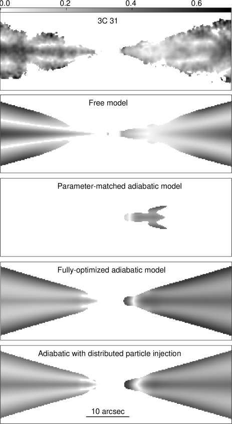
Figure 8: Grey-scale representations of the degree of polarization. The grey-scale runs from $p$ = 0 to $p$ = 0.7, as indicated by the labelled wedge. The panels extend $\pm$27 arcsec from the nucleus and the angular scale is indicated by the labelled bar. From the top: observations; free SSL model; parameter-matched adiabatic model; fully-optimized adiabatic model; adiabatic model with distributed particle injection. The initial conditions for the adiabatic models are set at the boundary between the inner and flaring regions. No emission is calculated for the adiabatic models within 2.5 arcsec of the nucleus.

Figure 9: Profiles of total intensity along the jet axes at a resolution of 0.75 arcsec FWHM. Full line: observations; short dashes: free SSL model; dots: parameter-matched adiabatic model; long dashes: fully-optimized adiabatic model; dash-dots: adiabatic model with distributed particle injection. The initial conditions for the adiabatic models are set at the boundary between the inner and flaring regions, so their profiles are plotted only for the outer and flaring regions ($>$2.5 arcsec from the nucleus).

The parameter-matched model fails because there is insufficient deceleration to counteract adiabatic losses resulting from the rapid expansion of the jets in the flaring region, even when field amplification by velocity shear is taken into account. There is also insufficient shear to counteract the effects of expansion at the edges of the jets, leading to a transverse apparent field there. The fully-optimized model fits much better, but has two main problems. First, it requires an extremely rapid deceleration in the flaring region: the initial on-axis velocity $\beta_{1}$ is in the range 0.93 – 0.99 for any $\theta$ and the corresponding velocity at the edge of the jet is ≳0.7, so high sidedness ratios are inevitable. Second, as in the outer region, the polarization data require far larger a change in the ratio $B_{r}/B_{t}$ than is allowed in our axisymmetric, laminar adiabatic model: a significant radial field component must first be generated at the edge of the flaring region and then destroyed further from the nucleus.

The extremely high sidedness ratios required by the optimized adiabatic models are inconsistent with observations. To help adiabatic models fit the data using the more realistic velocity field of the free models, additional emissivity must be introduced in the flaring region, as we now discuss.

Figure 10: Contours of total intensity at a resolution of 0.25 arcsec FWHM. The panels cover $\pm$10 arcsec from the nucleus and the angular scale is indicated. The contour levels are $-$1, 1, 2, 4, 8, 16, 32 $\times$ 30 $\mu$Jy/beam area. From the top: observations; free SSL model; parameter-matched adiabatic model; fully-optimized adiabatic model; adiabatic model with distributed particle injection. As the adiabatic models have initial conditions set at the boundary between the inner and flaring regions, no emission is calculated for the inner jet region ($<$2.5 arcsec from the nucleus).

Table 4: Fitted parameters for models with initial conditions at the boundary between the inner and flaring regions ($\bar{r}=r_{1}$). Note that $\theta$ and the velocity field are fixed for the particle-injection model; its remaining parameters are optimized.

Quantity	Parameter-	Fully-	Particle
	matched	optimized	injection
Angle to line of sight
$\theta$ (degrees)	51.4	55.0	51.4
Velocity field
On-axis velocities
$\beta_{1}$	0.76	0.99	0.76
$\beta_{0}$	0.54	0.77	0.54
$\beta_{f}$	0.27	0.40	0.27
Edge velocities
$v_{1}$	0.97	0.93	0.97
$v_{0}$	0.63	0.30	0.63
velocity exponent $H$	8.82	2.00	8.82
Emissivity profile
Edge emissivity $\bar{e}$	0.37	0.05	0.18
Radial/toroidal field ratios
On-axis $\bar{j}_{\rm cen}$	0.0	0.76	0.81
Edge $\bar{j}_{\rm out}$	0.78	0.42	0.42
Index $p$	0.41	1.50	0.62
Longitudinal/toroidal field ratios
On-axis $\bar{k}_{\rm cen}$	1.17	4.97	3.01
Edge $\bar{k}_{\rm out}$	1.17	2.65	3.01
Index $q$	0.0	3.96	0.0
Particle injection parameters
Cut-off $\rho_{\rm inj}$ (kpc)			2.16
Exponent $Q$			-4.71
Normalization $\Delta_{0}$			84.5
Goodness of fit
$\chi^{2}_{\rm red}$	30.4	4.65	4.92

5.3 Particle injection

It is clear from the earlier discussion that processes other than adiabatic evolution in an axisymmetric, laminar velocity field must be important in the flaring region of 3C 31 and may also have some effect at the start of the outer region. A process that locally increases the emissivity is clearly needed to compensate adiabatic expansion losses in the flaring region. Our modelling approach lets us estimate the rest-frame emissivity and the field-component ratios, but it cannot disentangle the roles of particles and magnetic field in the absence of any constraint from inverse-Compton emission. The observation of X-ray emission from the inner and flaring regions shows that fresh relativistic particles must be injected there, as the synchrotron lifetimes of electrons radiating at these frequencies are $\sim$10’s of years (Hardcastle et al., 2002). We therefore investigate a simple, but self-consistent physical model in which new (e.g. reaccelerated) particles with an energy distribution $\Delta n(E)dE\propto E^{-(2\alpha+1)}dE$ are added in a distributed fashion over the flaring region and then evolve adiabatically. We again fix the angle to the line of sight and velocity field at the best-fitting free model values, and assume that the magnetic field is frozen into the flow. We then optimize the initial conditions and particle injection function. We parameterize the particle injection as the ratio of the additional emissivity at position $(\rho,s)$ in the flaring region to its value on the same streamline at the start of the region, using the empirical relation:

$$\frac{\Delta\epsilon(\rho,s)}{\epsilon(r_{1},s)}=\Delta_{0}\left[1+\left(\frac{\rho-r_{1}}{r_{0}-r_{1}}\right)\right]^{-Q}$$

for $r_{1}\leq\rho\leq\rho_{\rm inj}$ (the emissivity function $\epsilon$ is defined in Section 2.1). This means that the transverse injection profile is a constant Gaussian function. The parameters $\Delta_{0}$, $Q$ and $\rho_{\rm inj}$ are optimized, with $\rho_{\rm inj}$ restricted to $r_{1}\leq\rho_{\rm inj}\leq r_{0}$.

The fit to the total-intensity distribution is generally good (Figs 7, 9 and 10), but the jet/counter-jet sidedness ratio close to the boundary between the inner and flaring regions is still significantly higher than is observed, despite the more modest velocity there. The reason is that the field is almost purely longitudinal, so the ratio is $\approx[(1+\beta\cos\theta)/(1-\beta\cos\theta)]^{3+2\alpha}$ (Begelman, 1993) rather than the usual $\approx[(1+\beta\cos\theta)/(1-\beta\cos\theta)]^{2+\alpha}$ appropriate for a field which is closer to isotropy. Given that the assumed magnetic-field evolution is unchanged, it is not surprising that the deficiencies in the polarization fits noted earlier are still present (Figs 7 and 8) and that an unrealistic field structure is required at the start of the flaring region. We do not, therefore, regard the high sidedness ratio as a significant problem for the model. The fit to the total intensity in the outer region is very similar to that of the parameter-matched model described in Section 4, as expected, so the need for some additional emissivity there remains. The overall fit is slightly worse than for the fully-optimized model ($\chi^{2}_{\rm red}=4.9$ compared with 4.7), but with 10 free parameters instead of 14. The optimized parameters for the particle-injection model are given in Table 4. Key implications are as follows:

1. Particle injection is required out to 6.4 arcsec (2.2 kpc) from the nucleus, i.e. only over the first half of the flaring region. In the second half of the region, the jet decelerates rapidly, thereby slowing the brightness decline predicted by adiabatic models. Further particle injection there would produce too slow a decline in brightness.

2. The injection rate decreases rapidly with distance from the nucleus within that region.

3. The emissivity everywhere in the flaring region is dominated by particles injected locally rather than those originating from the inner region.

Given the short synchrotron lifetimes of the electrons responsible for the high-energy emission, X-rays are likely to be produced close to the injection sites and the X-ray emissivity might therefore be expected to be roughly proportional to the injection function, $\Delta$, rather than to the radio emissivity. A comparison between the observed X-ray and radio emission profiles (Hardcastle et al. 2002, LB) and a model profile derived on this assumption (Fig. 11) supports this idea. The brightest X-ray emission comes from the inner 2.5 arcsec of the jet, which we have not modelled, but for which non-adiabatic evolution is clearly required (Section 5.1). In the first half of the flaring region, where we infer the need for significant particle injection, there is indeed evidence for more X-ray emission than in the outer half of the region, where injection is not required. The X-ray data in the flaring region are, however, too noisy to be sure whether the ratio of X-ray to radio emission changes within this region as our particle-injection model predicts. We also note that high-resolution studies of X-ray and radio emission from jets have shown that both may be highly inhomogeneous, with a complex mutual relationship (Hardcastle et al., 2003; Wilson & Yang, 2002).

If particles are indeed injected without much modifying the magnetic field, the ratio of particle to field energy is likely to increase (by an amount which we cannot estimate without a proper description of the injection mechanism). We would not, therefore, expect equipartition between field and particle energy everywhere in the flaring region, even if it holds in some locations. The region where we infer significant particle injection is also where the expansion rate of the jet is increasing (Fig. 3) and is where Laing & Bridle (2002b) inferred a significant over-pressure (Fig. 11b). The internal pressure significantly exceeds not only the external gas pressure, but also the synchrotron minimum pressure, so quite large deviations from equipartition could occur between 2.5 and $\approx$5 arcsec from the nucleus. In any case, we know that the magnetic field component ratios change in a way which is inconsistent with flux freezing in a laminar velocity field, so it is very likely that amplification of the field also occurs.

All of these results are consistent with injection (or reacceleration) of radiating particles over a wide energy range in the first half of the flaring region. The X-ray-emitting particles have extremely short synchrotron lifetimes and radiate where they are injected, whereas the lower-energy, radio-emitting particles suffer mainly adiabatic losses and radiate over the outer parts of the jet, as we have calculated. A quantitative study of the acceleration and energy-loss processes over the entire energy spectrum is outside the scope of the present paper.

Figure 11: Profiles of X-ray and radio emission and pressure along the axis of the main jet. (a) Flux-density profiles (on arbitrary scales) derived as in Fig. 3 of Hardcastle et al. (2002) by integration in boxes of size 0.3 $\times$ 2 arcsec² (short axis along the jet) on images of resolution 0.6 arcsec FWHM. Points: observed X-ray emission (Hardcastle et al., 2002); dashed line: observed radio emission (LB); full line: predicted X-ray emission profile for the flaring region alone, as described in the text. Note that the radio profile is derived from an image at a lower resolution than that used to make the equivalent plot in Hardcastle et al. (2002) in order to match the Chandra point-spread function as closely as possible. (b) Profiles of the internal (full), external (dashed) and synchrotron minimum (dotted) pressures from our conservation-law analysis (Laing & Bridle 2002b, Fig. 4, but projected onto the plane of the sky). The vertical dotted lines mark the extent of the flaring region as defined by LB and in Section 3.2.

6 Summary and Conclusions

We have investigated the hypothesis that the radio jets in 3C 31 can be modelled as adiabatic, decelerating, relativistic flows. Our technique has several advantages over previous work in: modelling linear polarization as well as total intensity; including the effects of velocity shear; taking account of anisotropic emission in the rest frame and fitting to two-dimensional images rather than to longitudinal profiles.

We have found that optimized adiabatic models give a fair description of the observed brightness and polarization distributions in the outer parts of the modelled region. Their fit to the data is inferior to that of the free models of LB, but is obtained with many fewer free parameters. The adiabatic models cannot describe the inner or flaring regions of the jets in 3C 31, however: the predicted distributions of total intensity and linear polarization are inconsistent with those observed. In the innermost region, the jets are clearly non-adiabatic unless the emission comes primarily from a part of the jet volume which is not expanding with distance from the nucleus (we do not resolve the region transversely). In the flaring region, a much higher initial velocity is required than is allowed by our measurements of jet/counter-jet sidedness ratio. The emission in this region is well resolved, and comes from the entire jet volume.

We have shown that a modified adiabatic model can still be fitted to the total intensity in this region if we add distributed injection of relativistic particles which then evolve adiabatically; the region where these particles must be injected is also one where there is independent evidence for recent particle acceleration from the detection of X-ray synchrotron radiation (Hardcastle et al., 2002) and of a local over-pressure in the jet from dynamical arguments (Laing & Bridle, 2002b).

While the total intensity distributions in the jet and counter-jet of 3C 31 can be reproduced satisfactorily by decelerating adiabatic jet models with particle injection in the flaring region, the polarization data (degree of linear polarization and apparent magnetic field direction) cannot. The apparent magnetic field configuration contains several features that are qualitatively incompatible with adiabatic evolution of all the field components in laminar-flow models, even in the presence of a velocity shear. We infer that the departures from adiabatic conditions in 3C 31 must also include deviations either from the flux-freezing description of the magnetic fields or from a laminar, axisymmetric velocity field. The free models of LB achieved better consistency with the observed polarization structure by allowing the field to become roughly isotropic at the edges of the jet in the flaring region. This could be achieved by a turbulent velocity component even if the field is frozen into the flow, in which case the resulting shear would also contribute to the enhancement in emissivity required to fit the adiabatic models in the flaring region. Processes such as dynamo action or field-line reconnection might also be significant.

More detailed analysis of the particle injection process inferred for the flaring region would benefit from more sensitive X-ray, optical and infra-red data and higher-resolution radio observations of this region, i.e. from deeper exposures with Chandra and HST and from deep higher-resolution polarimetry with the EVLA. Improved knowledge of the intensity and apparent magnetic field structures within this region might also assist development of models for the magnetic field microphysics in this region of the 3C 31 jet, which all of our analysis suggests is crucial in determining the deceleration dynamics of the jet, and its brightness and polarization properties further from the nucleus.

References

- (1)
- Baum et al. (1997) Baum, S.A., O’Dea, C.P., Giovannini, G., Biretta, J., Cotton, W.D., de Koff, S., Feretti, L., Golombek, D., Lara, L., Macchetto, F.D., Miley, G.K., Sparks, W.B., Venturi, T., Komissarov, S.S. 1997, ApJ, 483, 178 (erratum ApJ, 492, 854)
- Begelman (1993) Begelman, M.C., 1993, in Röser, H.-J., Meisenheimer, K., eds, Lecture Notes on Physics 421, Jets in Extragalactic Radio Sources. Springer-Verlag, Berlin, p. 145
- Begelman et al. (1984) Begelman, M.C., Blandford, R.D., Rees, M.J., 1984, Rev. Mod. Phys., 56, 255
- Bicknell (1984) Bicknell, G. V., 1984, ApJ, 286, 68
- Bicknell (1986) Bicknell, G. V., 1986, ApJ, 300, 591
- Bondi et al. (2000) Bondi, M., Parma, P., de Ruiter, H.R., Laing, R.A., Fomalont, E.B., 2000, MNRAS, 314, 11
- Burch (1979) Burch, S., 1979, MNRAS, 187, 187
- De Vaucouleurs et al. (1991) De Vaucouleurs, G., De Vaucouleurs, A., Corwin, H.G. Jr., Buta, R., Paturel, G., Fouque, P., Third Reference Catalogue of Bright Galaxies, Springer-Verlag, New York
- Fanaroff & Riley (1974) Fanaroff, B.L., Riley, J.M., 1974, MNRAS, 167, 31P
- Fanti et al. (1982) Fanti, R., Lari, C., Parma, P., Bridle, A.H., Ekers, R.D., Fomalont, E.B., 1982, A&A, 110, 169
- Feretti et al. (1999) Feretti, L., Perley, R., Giovannini, G., Andernach, H., 1999, A&A, 341, 29
- Hardcastle et al. (2002) Hardcastle, M.J., Worrall, D.M., Birkinshaw, M., Laing, R.A., Bridle, A.H., 2002, MNRAS, 334, 182
- Hardcastle et al. (2003) Hardcastle, M.J., Worrall, D.M., Kraft, R.P., Forman, W.R., Jones, C., Murray, S.S., 2003, ApJ, 593, 169
- Huchra et al. (1999) Huchra, J.P., Vogeley, M.S., Geller, M.J., 1999, ApJS, 121, 287
- Laing (1981) Laing, R.A., 1981, ApJ, 248, 87
- Laing (2002) Laing, R.A., 2002, MNRAS, 329, 417
- Laing & Bridle (2002a) Laing, R.A., Bridle, A.H., 2002a, MNRAS, 336, 328 (LB)
- Laing & Bridle (2002b) Laing, R.A., Bridle, A.H., 2002b, MNRAS, 336, 1161
- Laing et al. (1999) Laing, R.A., Parma, P., de Ruiter, H.R., Fanti, R., 1999, MNRAS, 306, 513
- Laing et al. (2004) Laing, R.A., Parma, P., Bridle, A.H., Feretti, L., Giovannini, G., Murgia, M., Perley, R.A., 2004, MNRAS,
- Matthews & Scheuer (1990) Matthews, A.P., Scheuer, P.A.G., 1990, MNRAS, 242, 616
- Smith et al. (2000) Smith, R.J., Lucey, J.R., Hudson, M.J., Schlegel, D.J., Davies, R.L., 2000, MNRAS, 313, 469
- Wilson & Yang (2002) Wilson, A.S., Yang, Y., 2002, ApJ, 568, 133