Reconstructing the primordial power spectrum - a new algorithm

Abstract

We propose an efficient and model independent method for reconstructing the primordial power spectrum from Cosmic Microwave Background (CMB) and large scale structure observations. The algorithm is based on a Monte Carlo principle and therefore very simple to incorporate into existing codes such as Markov Chain Monte Carlo.

The algorithm has been used on present cosmological data to test for features in the primordial power spectrum. No significant evidence for features is found, although there is a slight preference for an overall bending of the spectrum, as well as a decrease in power at very large scales.

We have also tested the algorithm on mock high precision CMB data, calculated from models with non-scale invariant primordial spectra. The algorithm efficiently extracts the underlying spectrum, as well as the other cosmological parameters in each case.

Finally we have used the algorithm on a model where an artificial glitch in the CMB spectrum has been imposed, like the ones seen in the WMAP data. In this case it is found that, although the underlying cosmological parameters can be extracted, the recovered power spectrum can show significant spurious features, such as bending, even if the true spectrum is scale invariant.

1 Introduction

The present cosmological concordance model has been shown to describe all present data surprisingly well with only about six parameters [1, 2]. From a physics point of view it is based on reasonable assumptions, such as general relativity and forms of matter with constant equations of state, albeit the physical nature of both the dark matter and the dark energy remains unknown. The initial perturbation spectrum appears to be almost purely adiabatic, Gaussian and scale invariant. Furthermore a general framework for producing such fluctuations in the early universe, namely inflation, is known and well established. As long as the universe remains deeply within the slow-roll regime during inflation, and the inflaton remains weakly coupled, Gaussian quantum fluctuations are produced which eventually become the adiabatic metric fluctuations observed for instance in the cosmic microwave background. However, there are many reasons to believe that there are deviations from this behaviour during the inflationary epoch, and countless physical mechanisms have been investigated. In the simplest models the deviations from scale invariance are caused by non-zero derivatives of the inflaton potential. Depending on the exact inflation model this can produce a tilt in the spectrum, and in general one can expand the produced spectrum of metric fluctuations in a Taylor series around the scale-invariant Harrison-Zeldovich spectrum

$$\log P(k)=\log P(k_{0})+(n-1)\log\frac{k}{k_{0}}+\left.\frac{1}{2}\frac{d\,n}{d\,\log k}\right|_{k_{0}}\,\log^{2}\frac{k}{k_{0}}+\cdots$$ (1)

where the different terms in the expansion are related to the derivatives of the potential.

Within this framework it has to be assumed that the universe does not deviate significantly from slow-roll in the sense that the power series above converges, and higher order terms are very small.

However, the present cosmological data shows some indication that the second order term is not small compared with the first order term [3, 4, 5, 6, 7, 8, 9, 10], perhaps indicating that the above series expansion does not converge, and that slow-roll may not be a valid approximation.

If one does away with the assumption of slow-roll during the production of fluctuations then much more radical deviations from scale invariance can be achieved. If for instance there are phase transitions or resonant production of particles during inflation, then step-like features in the power spectrum can occur [11, 12, 13, 14, 15]. It is in fact possible that such a feature is seen in the CMB data at the very largest scales, where the level of fluctuations is significantly smaller than expected.

On a different note it is also possible that effects from Planck scale physics can show up during inflationary slow-roll which occurs at much lower energies and perturb the spectrum of fluctuations [16, 17, 18, 19, 20, 21, 22, 23, 24, 25, 26, 27], one possibility being a logarithmic modulation of the power spectrum. This can occur even if the slow-roll conditions are fulfilled.

It is of course possible to search for specific types of features predicted in a given type of model, such as steps, Gaussian peaks, or oscillations (see e.g. [28]). However, with such a plethora of different possibilities it would be highly desirable with a model-independent and robust method for searching for deviations from scale invariance in the power spectrum. Such a method should be able to naturally encompass the power-law spectra predicted by standard slow-roll, as well as the more radical features such as steps and bumps.

In the present paper we describe exactly such a method which is able to extract features in the underlying spectrum, using either CMB or large scale structure data. Furthermore it is very easy to implement in existing software for cosmological parameter estimation.

In section 2 we describe general features of likelihood analysis, as well as the present cosmological data. In sections 3 and 4 we describe the spectrum reconstruction algorithm and use it on present cosmological data to search for features. In section 5 we go on to test the algorithm against mock data from future CMB experiments such as the Planck Surveyor. In section 6 we test how systematic errors in the $C_{l}$ data can affect parameter estimation and spectrum recovery. To that end we insert a Gaussian feature directly into the mock CMB data and do likelihood analysis on this modified data. Finally section 7 contains a discussion and conclusion.

2 Likelihood analysis

For calculating the theoretical CMB and matter power spectra we use the publicly available CMBFAST package [29]. As the set of cosmological parameters other than those related to the primordial spectrum we choose the minimum standard model with 4 parameters: $\Omega_{m}$, the matter density, the curvature parameter, $\Omega_{b}$, the baryon density, $H_{0}$, the Hubble parameter, and $\tau$, the optical depth to reionization. We restrict the analysis to geometrically flat models $\Omega=\Omega_{m}+\Omega_{\Lambda}=1$. When using large scale structure data we use the bias parameter, $b$, as a free parameter, which is a conservative, but well motivated choice.

parameter	prior
$\Omega_{m}$	$0.28\pm 0.14$ (Gaussian)
$h$	$0.72\pm 0.08$ (Gaussian)
$\Omega_{b}h^{2}$	$0.014-0.040$ (Top Hat)
$\tau$	$0-1$ (Top hat)
$b$	free

Table 1: The different priors on parameters used in the likelihood analysis. Parameters related to the power spectrum are not tabulated here.

In this numerical likelihood analysis we use the free parameters discussed above with certain priors determined from cosmological observations other than CMB and LSS. In flat models the matter density is restricted by observations of Type Ia supernovae to be $\Omega_{m}=0.28\pm 0.14$ [30]. Furthermore, the HST Hubble key project has obtained a constraint on $H_{0}$ of $72\pm 8\,\,{\rm km}\,{\rm s}^{-1}\,{\rm Mpc}^{-1}$ [31]. A summary of the priors can be found in table 1. The actual marginalization over parameters was performed using a simulated annealing procedure [32].

2.1 Cosmological data

Large scale structure – At present there are two large galaxy surveys of comparable size, the Sloan Digital Sky Survey (SDSS) [33, 1] and the 2dFGRS (2 degree Field Galaxy Redshift Survey)[34] Once the SDSS is completed in 2005 it will be significantly larger and more accurate than the 2dFGRS. At present the two surveys are, however, comparable in precision and in the present paper we use data from the 2dFGRS.

Tegmark, Hamilton and Xu [35] have calculated a power spectrum, $P(k)$, from this data, which we use in the present work. The 2dFGRS data extends to very small scales where there are large effects of non-linearity. Since we only calculate linear power spectra, we use (in accordance with standard procedure) only data on scales larger than $k=0.2h\,\,{\rm Mpc}^{-1}$, where effects of non-linearity should be minimal (see for instance Ref. [1] for a discussion). Making this cut reduces the number of power spectrum data points to 18.

CMB – The CMB temperature fluctuations are conveniently described in terms of the spherical harmonics power spectrum $C_{l}\equiv\langle|a_{lm}|^{2}\rangle$, where $\frac{\Delta T}{T}(\theta,\phi)=\sum_{lm}a_{lm}Y_{lm}(\theta,\phi)$. Since Thomson scattering polarizes light there are also power spectra coming from the polarization. The polarization can be divided into a curl-free $(E)$ and a curl $(B)$ component, yielding four independent power spectra: $C_{T,l},C_{E,l},C_{B,l}$ and the temperature $E$-polarization cross-correlation $C_{TE,l}$.

The WMAP experiment have reported data only on $C_{T,l}$ and $C_{TE,l}$, as described in Ref. [36, 2, 3, 37]

We have performed the likelihood analysis using the prescription given by the WMAP collaboration which includes the correlation between different $C_{l}$’s [36, 2, 3, 37]. Foreground contamination has already been subtracted from their published data.

In parts of the data analysis we also add other CMB data from the compilation by Wang et al. [38] which includes data at high $l$. Altogether this data set has 28 data points.

3 Reconstructing the power spectrum in bins

One method which has often been used to search for power spectrum features is to bin the spectrum into $N$ bins in $k$-space and then calculate what could be called a band amplitude in each of the bins [39, 40]. This is the crudest possible model and does not yield a continuous power spectrum. While there are models prediction such features they do not generally appear.

Another method is to do linear interpolation between the bin amplitudes. This was for instance done in the work by Bridle et al. [41] on the WMAP+2dF data (see also [42]). In this paper a parametrization was used where power at a given $k$ was

$$P(k)=\cases{\frac{(k_{i+1}-k)b_{i}+(k-k_{i})b_{i+1}}{k_{i+1}-k_{i}}&for $k_{i}<k<k_{i+1}$\cr b_{n}&for $k>k_{n}$},$$ (2)

where $b_{i}$ are the bin amplitudes and $k_{i}$ the bin positions.

However, this parametrization has the disadvantage that is does not fit a simple power-law spectrum. While the amplitude at each bin point can fit an overall power-law, the linear interpolation between bin points can only fit a simple power law if $n=1$.

The method we use for binning is therefore slightly different. We choose a $k_{\rm min}$ which is smaller than the minimum used in actual calculations (typically $k_{\rm min}=10^{-5}\,h$/Mpc) and $k_{\rm max}$ so that it is higher than the largest value used (typically $k_{\rm max}=1\,h$/Mpc). From the number of bins $N$ we then calculate $N+1$ points in $k$-space which are logarithmically spaced, i.e.

$$k_{i}=k_{\rm min}\left(\frac{k_{\rm max}}{k_{\rm min}}\right)^{i/N}\,\,\,\,,\,\,\,\,i=0,...,N$$ (3)

At each of these points there is a power spectrum amplitude, $A_{i}=\log(P(k_{i}))$. From this set of $N+1$ points linear interpolation is done in logarithmic space

$$A(k)=\cases{A(k_{0})&$k<k_{\rm min}$\cr A(k_{i})+(\log(k)-\log(k_{i}))\frac{A_{i+1}-A_{i}}{\log(k_{i+1})-\log(k_{i})}&$k_{\rm min}<k<k_{\rm max}$\cr A(k_{N})&$k>k_{\rm max}$}$$ (4)

This particular type of interpolation has the advantage that it has the simple power law spectrum as a special case. With this choice of binning there are $N+1$ free parameters (amplitudes) which can either be chosen using a Monte Carlo type algorithm or calculated on a grid. However, for large $N$ grid based methods become unfeasible.

The question is then how to judge whether adding more bins effectively improves the fit. $\chi^{2}$ in itself is not a good measure of whether the agreement with data is improved by increasing the number of bins because the effective number of degrees of freedom of the system changes when the number of bins changes. Instead we use the Goodness-of-Fit (GoF), defined as the probability of $\chi^{2}$ being larger than the obtained value by pure chance alone

$${\rm GoF}=\frac{1}{\Gamma(\nu/2)}\int_{\chi^{2}/2}^{\infty}e^{-t}t^{\nu/2-1}dt,$$ (5)

where $\nu$ is the effective number of degrees of freedom.

As long as the GoF increases when $N$ increases then there is a preference in the data for a feature or slope of some kind. Therefore the algorithm should be run with increasing $N$ until the GoF no longer increases. When the spectrum reconstruction has converged the GoF will actually decrease with increasing $N$ because $\nu$ increases.

Note that we do not calculate error bars on the bin amplitudes for each $N$. Rather the analysis can effectively be seen as a likelihood analysis in terms of a single parameter $N$, where all other parameters are marginalized over. However, as described above it is slightly different from a normal likelihood analysis because the number of degrees of freedom, $\nu$, changes with $N$.

It should be noted here that there is a radically different method for reconstructing the primordial power spectrum from CMB observations which relies on the fact that for constant cosmological parameters, the $C_{l}$ spectrum can be inverted to find $P(k)$ [43, 44]. However, the weakness of the method is that since any reasonable likelihood calculation must vary the cosmological parameters to find the best fit, spurious features can occur in the extracted power spectrum. Another possibility is to replace the binning with some other weighing, such as using a wavelet method [45, 46, 47]. In this latter case one estimates the amplitudes of a given number of basis functions. If these are chosen optimally then the method can be very powerful in picking up localized features in the power spectrum [46].

3.1 Application to present data

As a particular example we have used the binning method described here on current cosmological data.

We divide the likelihood analysis into two parts:
a) WMAP data only (referred to as WMAP only)
b) WMAP + Wang et al. + 2dFGRS data (referred to as ”all data”)
The results can be seen in Table 2, as well as in figures 1 and 2. From Table 2 we note that the GoF is quite poor for the WMAP data, a fact which is well known and ascribable to the fact that there are localized glitches in the power spectrum. While the physical meaning of these glitches is not yet fully understood it is likely that they have to do with the power spectrum reconstruction from the CMB maps, and not with any fundamental physics effect.

What is perhaps more interesting is that the application of the spectrum reconstruction algorithm does not lead to any significant improvement in the GoF. In most cases the $\chi^{2}$ value is almost unchanged.

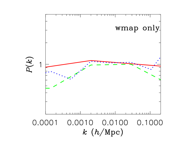
Figure 1: Reconstructed best fit power spectra to the WMAP data from the fixed bin algorithm. The full line is for $N=2$, the dashed for $N=4$, and the dotted for $N=8$.

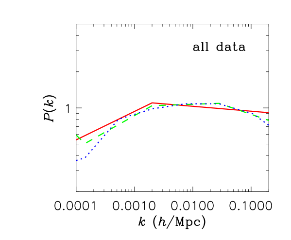
Figure 2: Reconstructed best fit power spectra to all present data from the fixed bin algorithm. The full line is for $N=2$, the dashed for $N=4$, and the dotted for $N=8$.

From figures 1 and 2 it is clear, however, that the data shows a slight preference for a negative running of the effective spectral index, i.e. the spectrum has an overall negative curvature. Exactly the same is also found in studies of the power spectrum within the slow roll approximation.

The spectrum reconstruction also finds that there is a dip in power around the scale of the lowest measurable multipoles. From the rough relation $l\sim 2kcH_{0}^{-1}$ (which applies exactly only to the flat, pure CDM model), we find that there some indication in the data for a dip around $k=0.001\,h$/Mpc, corresponding to $l\sim 5-10$. This again corresponds quite well to what is found in other studies [48, 49, 50, 51, 52, 53].

On the other hand, even though this seems like a pronounced effect in $P(k)$, the corresponding $C_{l}$ spectra shown in figure 3 are almost identical at low multipoles.

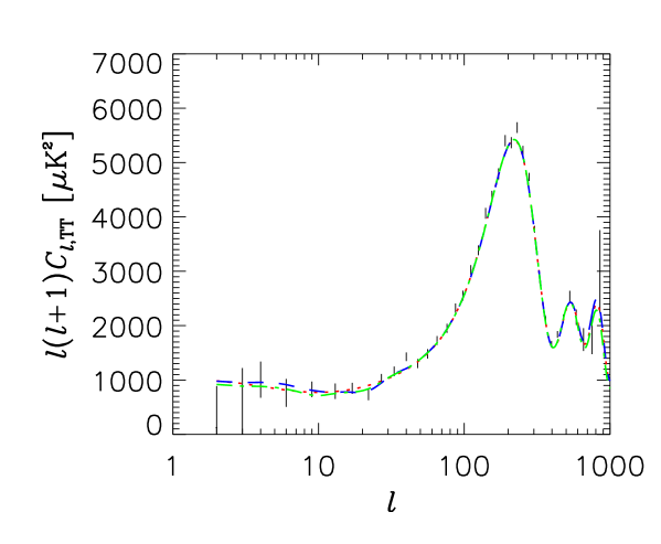
Figure 3: The temperature (TT) power spectra for the best fit models to the WMAP only data. The solid line is for $N=2$, the dashed for $N=4$, and the dotted for $N=8$. The black lines are the binned WMAP data.

One might wonder why this is the case when the fit would obviously be better if power was significantly reduced on small scales. The answer is that it is not possible to lower the amplitude of the $TT$ spectrum at small multipoles by changing the underlying power spectrum without doing the same to the $TE$ spectrum. This on the other hand fits well with a high amplitude at low multipoles, something which is usually ascribed to a high optical depth. This effect on the two different spectra at low multipoles can be seen in figure 4

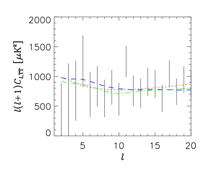
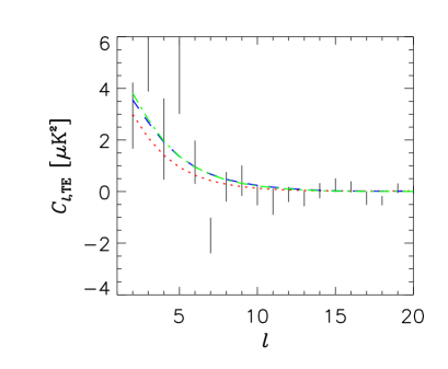
Figure 4: The temperature (TT) and temperature-polarization (TE) power spectra for the best fit models to the WMAP only data. The solid line is for $N=2$, the dashed for $N=4$, and the dotted for $N=8$. Only the low-$l$ parts of the spectra are shown. The black lines are the WMAP data.

The end result is that the overall best fit with regards to the power spectrum is one where there is a small decrease in amplitude at low $l$, but not sufficiently large that the $TE$ spectrum becomes inconsistent with data.

	WMAP data only		all data
$N$	$\chi^{2}$	GoF	$\chi^{2}$	GoF
2	1431.08	0.0432	1465.89	0.0742
4	1429.58	0.0422	1460.46	0.0836
8	1429.19	0.0364	1459.62	0.0745

Table 2: The smallest $\chi^{2}$ recovered for the fixed bin algorithm, based on the given data set. The Goodness-of-Fit (GoF) is defined in Eq. (5).

4 The sliding bin method

In the previous section we discussed a model independent way of searching for power spectrum variations and used it on present cosmological data. However, the binning in $k$-space was chosen a priori, a fact which can render the method almost useless in some instances. One example is the possibility of a step-like feature in the power spectrum. Such an abrupt feature cannot be fitted by the algorithm presented in the previous section, unless the number of bins is taken to be very large.

Of course one could search for steps in the spectrum by doing a new, independent scan of parameter space using the step height and location as free parameters. This method was for instance used by Bridle et al. [41] to search for various kinds of spectral effects in the present cosmological data.

However, it is clearly desirable to have a robust and more general method for searching for spectral deviations. A natural step is to allow the binning in $k$ to be free variables. Here we propose one such method which is simple to implement and fits extremely well with Monte Carlo based algorithms such as MCMC [54, 55] or simulated annealing [32].

The method goes as follows:

a)	Choose the number of $k$-space bins. This must now be a power of 2
	(i.e. 2, 4, 8, 16, …).
b) As in the previous algorithm calculate $N+1$ amplitudes.
c) Choose the lowest and highest $k$ values as fixed numbers. These should be chosen
	so that $k_{\rm min}$ is smaller than the minimum used in actual calculations and $k_{\rm max}$
	so that it is higher than the largest value used.
d) Start dividing up $k$-space. First choose one $k$-value, $k_{1}$, at random between
	the starting points with a flat prior so that $k_{1}=\alpha_{1}(k_{\rm max}-k_{\rm min})+k_{\rm min}$,
	where $\alpha_{1}\in[0,1]$ is a random number provided by for instance the MCMC
	algorithm. Next, choose a $k_{2}$ in the same way at random between $k_{\rm min}$ and $k_{1}$,
	and a $k_{3}$ between $k_{1}$ and $k_{\max}$.
e) Continue this iterative procedure until $N-1$ values have been chosen.
	This requires $\log(N)/\log(2)$ steps of the type described in d).
f) Now sort all of the $k$-values in increasing order, including $k_{\rm min}$ and $k_{\rm max}$. This
	yields $N+1$ $k$-values which correspond to the $N+1$ amplitudes generated in b)

Even though the method at first may seem confusing because it relabels $k$-values, it in fact ensures that the $N+1$ tuple of $k$-values is always in increasing order, but with varying spacing. It is not important at all how the individual $k$-values are labelled while they are generated, as long as they are sorted in increasing order at the end.

Altogether there are now $2N+2$ numbers related to the binning and the amplitudes. $2N$ of these are random numbers, only the $k_{\rm min}$ and $k_{\rm max}$ are fixed numbers.

The $2N$ numbers can be generated for instance by a Monte Carlo based algorithm or they can be run on a grid. The algorithm is straightforward to incorporate into existing likelihood calculators such as Markov Chain Monte Carlo, it just introduces $2N$ new “cosmological parameters” into the analysis.

By this method it is for instance possible in principle to sample a step-like feature perfectly with $N=4$ (but not with N=2).

Apart from sliding bins the method is completely identical to that described in the previous section. However, it has the very big advantage of being able to detect narrow features of almost any shape and location in the primordial power spectrum.

4.1 Application to present data

The results of likelihood analyses with $N=2,4,$ and 8 are shown in Table 3. From this it is clear that when applied to the present cosmological data the algorithm does not perform significantly better than the crude binning algorithm of the previous section. This is not surprising since there are no detectable features of any significance in the present data. For a given $N$ the obtained $\chi^{2}$ is in each case slightly better than what is obtained with the fixed bins method of the previous section. However, the Goodness-of-Fit is actually worse because there are $2N$ free parameters in the sliding bins method and only $N+1$ in the fixed bins method.

Figures 5 and 6 show the reconstructed spectra. As in the case of the algorithm with fixed binning there is indication of an overall bending of the spectrum, corresponding to a negative curvature. Furthermore there is indication of a dip in power at large scales. For the WMAP-only data the dip is at $k=0.001-0.002\,h$/Mpc, corresponding roughly to $l\sim 10$, whereas for all data combined the dip occurs at a scale corresponding to roughly $l=2-4$.

However, as with the fixed binning algorithm there is no statistical evidence for features in the spectrum. The GoF is constant or decreases when $N$ increases, which indicates that there are no significant features hidden.

One other important feature should be noted, namely that there is apparently a rather large change in the derived power spectrum on large scales when including other data sets than WMAP. At first this may appear confusing because the other data sets are relevant only on smaller scales. However, the simulated annealing algorithm used is very powerful for finding the global extremum of a function, but it is not an MCMC type algorithm, i.e. it does not provide an estimate of the distribution of the function. Therefore no error bars are plotted in these figures. One should instead think of the analysis as a 1-parameter likelihood analysis, with $N$ being the free parameter. The actual spectra plotted in the figures are the best fit models only. Close to the horizon scale the error bars on the extracted spectrum are large and therefore the features appear more dramatic than they really are. Instead one should look at the Goodness-of-fit as a function of $N$, in which case there is no really significant evidence for features.

Even though the sliding bin method does not perform better than the fixed bin method for the present data, it performs extremely well when there are localized features in the spectrum, as will be demonstrated in the next section.

	WMAP data only		all data
$N$	$\chi^{2}$	GoF	$\chi^{2}$	GoF
2	1430.73	0.0421	1463.42	0.0779
4	1428.14	0.0397	1460.08	0.0759
8	1428.08	0.0282	1457.59	0.0620

Table 3: The smallest $\chi^{2}$ recovered from the sliding bin algorithm, based on the given data set. The Goodness-of-Fit (GoF) is defined in Eq. (5).

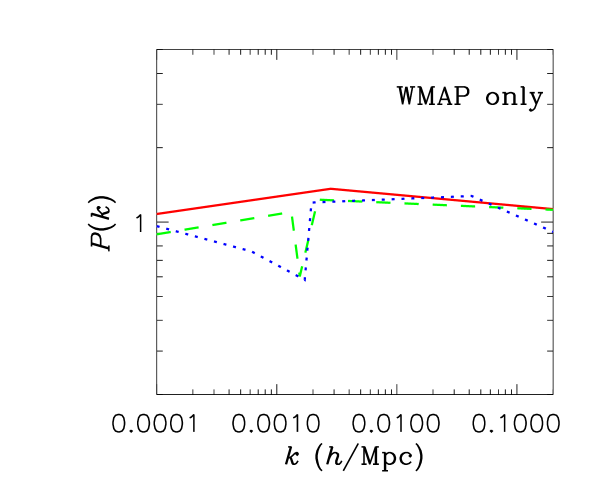
Figure 5: Reconstructed best fit power spectra to the WMAP data from the sliding bin algorithm. The full line is for $N=2$, the dashed for $N=4$, and the dotted for $N=8$.

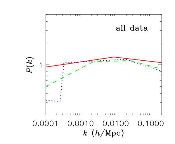
Figure 6: Reconstructed best fit power spectra to all present data from the sliding bin algorithm. The full line is for $N=2$, the dashed for $N=4$, and the dotted for $N=8$.

5 Testing the algorithm on mock CMB data

We have simulated a data set from the future Planck mission using the following very simple prescription: We assume it to be cosmic variance (as opposed to foreground) limited up to some maximum $l$-value, $l_{\rm max}$, which we take to be 2000. For the sake of simplicity we shall work only with the temperature power spectrum, $C_{T,l}$, in the present analysis. In fact the Planck detectors will be able to measure polarization as well as temperature anisotropies, but our simplification of using only $C_{T,l}$ will not have a significant qualitative impact on our conclusions. For a cosmic variance limited full sky experiment the uncertainty in the measurement of a given $C_{l}$ is simply

$$\frac{\sigma(C_{l})}{C_{l}}=\sqrt{\frac{2}{2l+1}}.$$ (6)

It should be noted that taking the data to be cosmic variance limited corresponds to the best possible case. In reality it is likely that foreground effects will be significant, especially at high $l$. Therefore, our estimate of the precision with which the oscillation parameters can be measured is probably on the optimistic side.

As the underlying cosmological model for all cases in this and the next section we choose a standard $\Lambda$CDM model with $\Omega_{0}=1$, $\Omega_{m}=0.3$, $\Omega_{b}=0.04$, $H_{0}=70\,\,{\rm km}\,{\rm s}^{-1}\,{\rm Mpc}^{-1}$, and $\tau=0$.

5.1 A step in the spectrum

As a test case we use a primordial power spectrum which has a step at $k=0.05h$/Mpc,

$$P(k)=\cases{1&for $k<0.05h$/Mpc\cr 1.3&for $k>0.05h$/Mpc}$$ (7)

In Table 4 we show the best fit $\chi^{2}$ obtained for $N=2,4,$ and 8. In this case the GoF increases dramatically with increasing $N$, indicating that there is a feature in the spectrum. From Figure 7 it can also be seen that the step is faithfully recovered by the algorithm. For $N=4$ it is located at the correct place in $k$-space, but is not quite sharp enough. For $N=8$ the step feature is recovered almost perfectly, except for a transient effect right at the edge. Such an effect is not surprising because the algorithm has to reproduce a discontinuity.

$N$	$\chi^{2}$	GoF
2	13038.78	$7.17\times 10^{-1590}$
4	2251.23	$2.80\times 10^{-5}$
8	2147.63	0.00442

Table 4: The smallest $\chi^{2}$ recovered from the model with a step-like feature. The Goodness-of-Fit (GoF) is defined in Eq. (5).

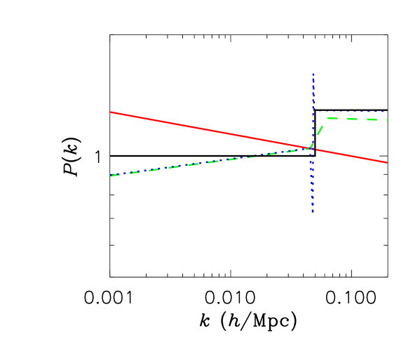
Figure 7: Reconstructed best fit power spectra to the underlying spectrum from Eq. (7). The full line is for $N=2$, the dashed for $N=4$, and the dotted for $N=8$. The thick (black) line is the power spectrum of the input model.

5.2 A Gaussian feature

The next case is a Gaussian suppression of the spectrum around $k=0.05h$/Mpc,

$$P(k)=1-\alpha\exp\left(-\frac{(\log(k)-\log(k_{b}))^{2}}{\beta^{2}}\right),$$ (8)

where we have taken $k_{b}=0.05h$/Mpc, $\alpha=0.7$, $\beta^{2}=0.1$.

In Table 5 the best fit $\chi^{2}$ and GoF are shown, again for $N=2,4,$ and 8. Figure 8 shows the recovered spectra.

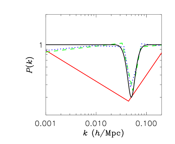
Figure 8: Reconstructed best fit power spectra to the underlying spectrum from Eq. (8). The full line is for $N=2$, the dashed for $N=4$, and the dotted for $N=8$. The thick (black) line is the power spectrum of the input model.

$N$	$\chi^{2}$	GoF
2	25109.22	$6.13\times 10^{-3928}$
4	2289.51	$2.27\times 10^{-6}$
8	2147.63	$2.82\times 10^{-5}$

Table 5: The smallest $\chi^{2}$ recovered from the model with a Gaussian feature. The Goodness-of-Fit (GoF) is defined in Eq. (5).

Not surprisingly the best fit even for $N=8$ is not tremendously good because it is inherently difficult to mimic a continuous feature in the spectrum by a sequence of lines.

However, the recovered $\chi^{2}$ and the reconstructed spectrum is much better than what a crude binning algorithm can do on the same data [40]. Furthermore the shape of the underlying spectrum is recovered nicely and unbiased. Finally, in figure 9 we show CMB spectra of the underlying theoretical spectra discussed in sections 5.1 and 5.2.

Figure 9: The CMB spectra of the two simulated data sets. The dashed line is for the model with a step, the dotted for the model with a Gaussian feature. The full line is for a model with the same cosmological parameters and a scale invariant spectrum.

6 Glitches in the CMB spectrum

As a last application we study what happens to spectrum estimation in the event where there are significant, but completely unphysical bumps on the $C_{l}$ spectrum. To do this we have generated a mock CMB data in the same manner as in the previous section for a completely scale invariant model ($n=1$), but on top of that we have added a Gaussian feature, so that the final $C_{l}$ in given in terms of the original $C_{l}$ as

$$C_{l,{\rm new}}=C_{l,{\rm old}}(1+0.2\exp(-(l-350)^{2}/5^{5}))$$ (9)

In figure 10 we show the two sets of mock CMB data. The left spectrum has the added Gaussian feature, while the right one is the original unperturbed mock spectrum.

The question is then to what extent the estimation, both of the spectrum and of the cosmological parameters, is perturbed by this feature.

In Table 6 it can be seen that the true, underlying parameters are not retrieved in the case with $N=2$. However, already for $N=4$ the cosmological parameters are estimated correctly. On the other hand, from figure 11 it can be seen that the extracted power spectrum is no longer the fully scale invariant $n=1$ Harrison-Zeldovich spectrum of the input model. Rather, the best fit model now shows a distinct bending. This shows that errors in the $C_{l}$ construction from the map in the form of bumps or glitches can lead to a biasing of the power spectrum estimation. Although the feature in the $C_{l}$ spectrum which is used here is significantly larger than the ones seen in the WMAP data (as can be seen from the fact that the $N=2$ model gives an exceedingly bad fit) it is quite possible to bias power spectrum estimation and make an underlying scale invariant spectrum look like it is bending.

The fact that the other cosmological parameters can be extracted with great precision is not too surprising. The reason is that parameters such as $\Omega_{m}$, $H_{0}$, and $\Omega_{b}$ all produce wide non-localized features in the spectrum. Therefore it is quite impossible to mimic a narrow Gaussian feature by a linear combination of changes in the underlying cosmological parameters.

Figure 10: The two sets of mock CMB data. The right figure shows the unperturbed observational data, whereas the left curve shows the data with a Gaussian peak added at $l=350$.

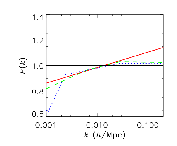
Figure 11: Reconstructed best fit power spectra to the underlying scale invariant spectrum, modified according to Eq. (9). The full line is for $N=2$, the dashed for $N=4$, and the dotted for $N=8$. The thick (black) line is the power spectrum of the input model.

$N$	$\chi^{2}$	GoF	$\Omega_{m}h^{2}$	$\Omega_{b}h^{2}$	h
2	3425.72	$6.97\times 10^{-80}$	0.179	0.0203	0.600
4	2133.43	0.0114	0.146	0.0199	0.706
8	2131.30	0.00885	0.146	0.0198	0.707

Table 6: The smallest $\chi^{2}$ recovered based on the modified spectrum from Eq. (9), as well as the best fit values of $\Omega_{m}h^{2}$, $\Omega_{b}h^{2}$, and $h$. The Goodness-of-Fit (GoF) is defined in Eq. (5).

6.1 A glitch at low $l$

Finally we have also tested the effect of having a glitch at lower $l$ in order to see whether that produces similar effects. We have added a glitch of the same magnitude and width as above, but at $l=40$.

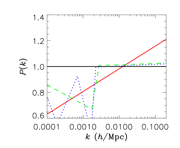
Figure 12: Reconstructed best fit power spectra to the underlying scale invariant spectrum, modified according to Eq. (9), but with the feature located at $l=40$. The full line is for $N=2$, the dashed for $N=4$, and the dotted for $N=8$. The thick (black) line is the power spectrum of the input model.

From figure 12 it can be seen that in this case the reconstructed spectrum also shows features. The main effect is at $k\sim 0.001h$/Mpc, corresponding to roughly $l\sim 40$, but here again there are features at larger scales as well. In general narrow features in the $C_{l}$ spectrum will not show up as narrow features in the reconstructed $P(k)$.

7 Discussion

We have developed an efficient and model-independent method for reconstructing the primordial power spectrum from cosmological observations of both CMB and large scale structure. This method has the major advantage that it can locate even narrow features in the spectrum very accurately. Furthermore the algorithm is very easy to implement in current likelihood calculators which are Monte Carlo based, although it can also be used in grid based algorithms.

We then tested the algorithm on current cosmological data and found, in accordance with numerous other studies, no significant evidence for any features in the primordial spectrum of fluctuations, $P(k)$. There is a slight preference for an overall negative curvature of the spectrum, corresponding to a negative running of the spectral index. However, the statistical significance is very low. Furthermore there is an indication of a break in the power spectrum at the very largest observable scales, corresponding to the dip in power at low $l$ seen by WMAP. Again, however, the statistical significance of this feature is very low.

In order to test the efficiency and robustness of the algorithm we then went on to use it on mock data from a future high-precision experiment such as the Planck Surveyor. Two cases were investigated, one with a step-like feature imposed, and one with a Gaussian suppression of the power spectrum. In both cases the algorithm was able to recover the true, underlying power spectrum very efficiently and with no biasing, something which would for instance be extremely difficult for algorithms with fixed bins.

Finally we tested the algorithm on a mock CMB spectrum, where a noise feature of Gaussian shape was imposed after the data was generated. The reason is that such glitches are seen in the present WMAP data, and it is of interest to know whether the true power spectrum, as well as other cosmological parameters can be safely recovered even if there are such spurious features present.

Running the algorithm we found that the cosmological parameters of the underlying model could be recovered safely, but that the extracted primordial spectrum no longer resembled to scale-invariant spectrum used to generate the data. Rather it showed a distinct bending. This means that care should be taken when extracting information on the primordial power spectrum, including such parameters as the running of the spectral index, from power spectra which show spurious, localized features in $l$-space.

References

- [1] M. Tegmark et al. [SDSS Collaboration], “Cosmological parameters from SDSS and WMAP,” astro-ph/0310723.
- [2] D. N. Spergel et al., “First Year Wilkinson Microwave Anisotropy Probe (WMAP) Observations: Determination of Cosmological Parameters,” Astrophys. J. Suppl. 148, 175 (2003) [astro-ph/0302209].
- [3] H. V. Peiris et al., “First year Wilkinson Microwave Anisotropy Probe (WMAP) observations: Implications for inflation,” Astrophys. J. Suppl. 148, 213 (2003) [astro-ph/0302225].
- [4] S. M. Leach and A. R. Liddle, “Constraining slow-roll inflation with WMAP and 2dF,” astro-ph/0306305.
- [5] A. Lue, G. D. Starkman and T. Vachaspati, “A post-WMAP perspective on inflation,” astro-ph/0303268.
- [6] V. Barger, H. S. Lee and D. Marfatia, “WMAP and inflation,” Phys. Lett. B 565, 33 (2003) [hep-ph/0302150].
- [7] W. H. Kinney, E. W. Kolb, A. Melchiorri and A. Riotto, “WMAPping inflationary physics,” hep-ph/0305130.
- [8] W. H. Kinney, A. Melchiorri and A. Riotto, “New constraints on inflation from the cosmic microwave background,” Phys. Rev. D 63, 023505 (2001) [astro-ph/0007375].
- [9] S. Hannestad, S. H. Hansen and F. L. Villante, “Probing the power spectrum bend with recent CMB data,” Astropart. Phys. 16, 137 (2001) [astro-ph/0012009].
- [10] S. Hannestad, S. H. Hansen, F. L. Villante and A. J. S. Hamilton, “Constraints on inflation from CMB and Lyman-alpha forest,” Astropart. Phys. 17, 375 (2002) [astro-ph/0103047].
- [11] A. A. Starobinsky, “Spectrum Of Adiabatic Perturbations In The Universe When There Are Singularities In The Inflation Potential,” JETP Lett. 55, 489 (1992) [Pisma Zh. Eksp. Teor. Fiz. 55, 477 (1992)].
- [12] D. J. H. Chung, E. W. Kolb, A. Riotto and I. I. Tkachev, “Probing Planckian physics: Resonant production of particles during inflation and features in the primordial power spectrum,” Phys. Rev. D 62, 043508 (2000) [hep-ph/9910437].
- [13] O. Elgaroy, S. Hannestad and T. Haugboelle, “Observational constraints on particle production during inflation,” JCAP 0309, 008 (2003) [astro-ph/0306229].
- [14] J. Barriga, E. Gaztanaga, M. G. Santos and S. Sarkar, “On the APM power spectrum and the CMB anisotropy: Evidence for a phase transition during inflation?,” Mon. Not. Roy. Astron. Soc. 324, 977 (2001) [astro-ph/0011398].
- [15] J. A. Adams, G. G. Ross and S. Sarkar, “Multiple inflation,” Nucl. Phys. B 503, 405 (1997) [hep-ph/9704286].
- [16] J. Martin and R. H. Brandenberger, Phys. Rev. D 63, 123501 (2001) [hep-th/0005209].
- [17] R. H. Brandenberger and J. Martin, Mod. Phys. Lett. A 16, 999 (2001) [astro-ph/0005432].
- [18] J. C. Niemeyer, Phys. Rev. D 63, 123502 (2001) [astro-ph/0005533].
- [19] R. Easther, B. R. Greene, W. H. Kinney and G. Shiu, Phys. Rev. D 64, 103502 (2001) [hep-th/0104102].
- [20] R. Easther, B. R. Greene, W. H. Kinney and G. Shiu, Phys. Rev. D 67, 063508 (2003) [hep-th/0110226].
- [21] U. H. Danielsson, Phys. Rev. D 66, 023511 (2002) [hep-th/0203198].
- [22] R. Easther, B. R. Greene, W. H. Kinney and G. Shiu, Phys. Rev. D 66, 023518 (2002) [hep-th/0204129].
- [23] G. L. Alberghi, R. Casadio and A. Tronconi, gr-qc/0303035.
- [24] J. Martin and R. Brandenberger, Phys. Rev. D 68, 063513 (2003) [hep-th/0305161].
- [25] L. Bergstrom and U. H. Danielsson, “Can MAP and Planck map Planck physics?,” JHEP 0212, 038 (2002) [hep-th/0211006].
- [26] O. Elgaroy and S. Hannestad, “Can Planck-scale physics be seen in the cosmic microwave background?,” astro-ph/0307011.
- [27] J. Martin and C. Ringeval, “Superimposed Oscillations in the WMAP Data?,” astro-ph/0310382.
- [28] O. Elgaroy, M. Gramann and O. Lahav, “Features in the primordial power spectrum: constraints from the CMB and the limitation of the 2dF and SDSS redshift surveys to detect them,” astro-ph/0111208.
- [29] U. Seljak and M. Zaldarriaga, “A Line of Sight Approach to Cosmic Microwave Background Anisotropies,” Astrophys. J. 469, 437 (1996) [astro-ph/9603033].
- [30] S. Perlmutter et al. [Supernova Cosmology Project Collaboration], “Measurements of Omega and Lambda from 42 High-Redshift Supernovae,” Astrophys. J. 517, 565 (1999) [astro-ph/9812133].
- [31] W. L. Freedman et al., Astrophys. J. Lett. 553, 47 (2001).
- [32] S. Hannestad, “Stochastic Optimization Methods For Extracting Cosmological Parameters From Cosmic Microwave Background Radiation Power Spectra,” Phys. Rev. D 61, 023002 (2000) [astro-ph/9911330].
- [33] M. Tegmark et al. [SDSS Collaboration], astro-ph/0310725.
- [34] M. Colless et al., “The 2dF Galaxy Redshift Survey: Final Data Release,” astro-ph/0306581.
- [35] M. Tegmark, A. J. S. Hamilton and Y. Xu, Mon. Not. Roy. Astron. Soc. 335, 887 (2002) [astro-ph/0111575].
- [36] C. L. Bennett et al., “First Year Wilkinson Microwave Anisotropy Probe (WMAP) Observations: Preliminary Maps and Basic Results,” Astrophys. J. Suppl. 148, 1 (2003) [astro-ph/0302207].
- [37] L. Verde et al., “First Year Wilkinson Microwave Anisotropy Probe (WMAP) Observations: Parameter Estimation Methodology,” Astrophys. J. Suppl. 148, 195 (2003) [astro-ph/0302218].
- [38] X. Wang, M. Tegmark, B. Jain and M. Zaldarriaga, “The last stand before MAP: cosmological parameters from lensing, CMB and galaxy clustering,” astro-ph/0212417.
- [39] Y. Wang, D. N. Spergel and M. A. Strauss, “Cosmology in the next millennium: Combining MAP and SDSS data to constrain inflationary models,” Astrophys. J. 510, 20 (1999) [astro-ph/9802231].
- [40] S. Hannestad, “Reconstructing the inflationary power spectrum from CMBR data,” Phys. Rev. D 63, 043009 (2001) [astro-ph/0009296].
- [41] S. L. Bridle, A. M. Lewis, J. Weller and G. Efstathiou, “Reconstructing the primordial power spectrum,” Mon. Not. Roy. Astron. Soc. 342, L72 (2003) [astro-ph/0302306].
- [42] Y. Wang and G. Mathews, “A measurement of the primordial power spectrum from Maxima and Boomerang Astrophys. J. 573, 1 (2002) [arXiv:astro-ph/0011351].
- [43] N. Kogo, M. Matsumiya, M. Sasaki and J. Yokoyama, “Reconstructing the primordial spectrum from WMAP data by the cosmic inversion method,” astro-ph/0309662.
- [44] M. Matsumiya, M. Sasaki and J. Yokoyama, “Cosmic Inversion II –An iterative method for reproducing the primordial spectrum from the CMB data–,” JCAP 0302, 003 (2003) [astro-ph/0210365].
- [45] P. Mukherjee and Y. Wang, “Wavelet Band Powers of the Primordial Power Spectrum from CMB Data,” Astrophys. J. 593, 38 (2003) [astro-ph/0301058].
- [46] P. Mukherjee and Y. Wang, “Direct Wavelet Expansion of the Primordial Power Spectrum: Results from Astrophys. J. 598, 779 (2003) [arXiv:astro-ph/0301562].
- [47] P. Mukherjee and Y. Wang, “Model-Independent Reconstruction of the Primordial Power Spectrum from WMAP Astrophys. J. 599, 1 (2003) [arXiv:astro-ph/0303211].
- [48] J. M. Cline, P. Crotty and J. Lesgourgues, “Does the small CMB quadrupole moment suggest new physics?,” JCAP 0309, 010 (2003) [astro-ph/0304558].
- [49] C. R. Contaldi, M. Peloso, L. Kofman and A. Linde, “Suppressing the lower Multipoles in the CMB Anisotropies,” JCAP 0307, 002 (2003) [astro-ph/0303636].
- [50] B. Feng and X. Zhang, “Double inflation and the low CMB quadrupole,” Phys. Lett. B 570, 145 (2003) [astro-ph/0305020].
- [51] G. Efstathiou, “A Maximum Likelihood Analysis of the Low CMB Multipoles from WMAP,” astro-ph/0310207.
- [52] G. Efstathiou, “The Statistical Significance of the Low CMB Mulitipoles,” astro-ph/0306431.
- [53] A. de Oliveira-Costa, M. Tegmark, M. Zaldarriaga and A. Hamilton, “The significance of the largest scale CMB fluctuations in WMAP,” astro-ph/0307282.
- [54] N. Christensen, R. Meyer, L. Knox and B. Luey, “II: Bayesian Methods for Cosmological Parameter Estimation from Cosmic Microwave Background Measurements,” Class. Quant. Grav. 18, 2677 (2001) [astro-ph/0103134].
- [55] A. Lewis and S. Bridle, “Cosmological parameters from CMB and other data: a Monte-Carlo approach,” Phys. Rev. D 66, 103511 (2002) [astro-ph/0205436].