A long, hard look at MCG–6-30-15 with XMM-Newton II: detailed EPIC analysis and modelling

Abstract

The bright Seyfert 1 galaxy MCG–6-30-15 has provided some of the best evidence to date for the existence of supermassive black holes in active galactic nuclei. Observations with ASCA revealed an X-ray iron line profile shaped by strong Doppler and gravitational effects. In this paper the shape of the iron line, its variability characteristics and the robustness of this spectral interpretation are examined using the long XMM-Newton observation taken in 2001. A variety of spectral models, both including and excluding the effects of strong gravity, are compared to the data in a uniform fashion. The results strongly favour models in which the spectrum is shaped by emission from a relativistic accretion disc. It is far more difficult to explain the $3-10{\rm\thinspace keV}$ spectrum using models dominated by absorption (either by warm or partially covering cold matter), emission line blends, curved continua or additional continuum components. These provide a substantially worse fit to the data and fail to explain other observations (such as the simultaneous BeppoSAX spectrum). This reaffirms the veracity of the relativistic ‘disc line’ interpretation. The short term variability in the shape of the energy spectrum is investigated and explained in terms of a two-component emission model. Using a combination of spectral variability analyses the spectrum is successfully decomposed into a variable power-law component (PLC) and a reflection dominated component (RDC). The former is highly variable while the latter is approximately constant throughout the observation, leading to the well-known spectral variability patterns. Consideration of the long term X-ray monitoring of MCG–6-30-15 by RXTE demonstrates that the long XMM-Newton observation sampled the ‘typical’ state of the source. These results and those of other analyses of the large XMM-Newton dataset are summarised and their implications for understanding this enigmatic source are discussed.

1 Introduction

X-ray spectroscopy holds great promise for probing physics close to the accreting black holes thought to power Active Galactic Nuclei (AGN) and Galactic Black Hole Candidates (GBHCs). The high X-ray luminosities observed from these systems are thought to be generated close to the black hole ($\mathrel{\hbox{\hbox to0.0pt{\hbox{\lower 4.0pt\hbox{$\sim$}}\hss}\hbox{$<$}}}100{\thinspace r_{\rm g}}$; where ${\thinspace r_{\rm g}}\equiv GM/c^{2}$ is the gravitational radius) where the effects of strong gravity, such as gravitational redshift and light bending, will imprint characteristic signatures on the emerging X-ray spectrum.

As it escapes towards the observer, the primary X-ray emission will interact with material in the innermost regions, modifying the observed X-ray spectrum. Reprocessing of the X-rays by an accretion disc will lead to a particular set of spectral features. Absorption, fluorescence, recombination, and Compton scattering in the surface layers of the X-ray illuminated disc produce a ‘reflection’ spectrum. Under a wide range of physical conditions the most prominent observables will be an emission line at $\approx 6.4{\rm\thinspace keV}$ (the iron K$\alpha$ fluorescence line) and a broad ‘hump’ in the spectrum which peaks in the range $20-40{\rm\thinspace keV}$ (e.g. Guilbert & Rees 1988; Lightman & White 1988; George & Fabian 1991; Matt, Perola & Piro 1991). Observations of Seyfert 1 galaxies with Ginga (Pounds et al. 1990; Nandra & Pounds 1994) demonstrated the simultaneous presence of a $\approx 6.4{\rm\thinspace keV}$ emission line and an up-turn in the spectrum above $\sim 10{\rm\thinspace keV}$, indicative of the reflection hump. The presence of the reflection hump has since been confirmed by CGRO (e.g. Zdziarski et al. 1995) and BeppoSAX (e.g. Perola et al. 2002).

The bright Seyfert 1 galaxy MCG–6-30-15 ($z=0.007749$) has received particular attention since ASCA observations revealed the presence of a broad, asymmetric emission feature at energies between $4-7{\rm\thinspace keV}$ identified with a highly broadened Fe K$\alpha$ emission line (Tanaka et al. 1995). Similar features were subsequently observed in other Seyfert 1 galaxies (Mushotzky et al. 1995; Nandra et al. 1997). The profile of the line can be explained in terms of fluorescent emission from the surface of an accretion disc extending down to $\mathrel{\hbox{\hbox to0.0pt{\hbox{\lower 4.0pt\hbox{$\sim$}}\hss}\hbox{$<$}}}6{\thinspace r_{\rm g}}$ about a supermassive black hole (SMBC): the relativistic ‘disc line’ model (Fabian et al. 1989; Stella 1990; Laor 1991). For comparison, the emission lines seen in other wavebands (e.g. broad optical lines) are thought to originate at distances $\mathrel{\hbox{\hbox to0.0pt{\hbox{\lower 4.0pt\hbox{$\sim$}}\hss}\hbox{$>$}}}10^{3}{\thinspace r_{\rm g}}$. The broad Fe K$\alpha$ line therefore potentially offers a powerful diagnostic of the physical conditions in the immediate environment of the black hole (see Fabian et al. 2000; Nandra 2001 and Reynolds & Nowak 2003 for recent reviews).

Repeated observations of MCG–6-30-15 with ASCA (Iwasawa et al. 1996, 1999; Shih et al. 2002), BeppoSAX (Guainazzi et al. 1999), RXTE (Lee et al. 1999, 2000; Vaughan & Edelson 2001), Chandra (Lee et al. 2002) and XMM-Newton (Wilms et al. 2001, hereafter W01, and Fabian et al. 2002, hereafter paper I) have confirmed the presence of the broad, asymmetric emission feature. However, while this is clearly not an artifact of any particular instrument or observation, there are uncertainties associated with the detailed modelling of the spectrum. The most challenging of these is that MCG–6-30-15, along with many other Seyfert 1s, shows complex absorption in its X-ray spectrum. This complicates the process of identifying the correct underlying continuum and thereby measuring the superposed line emission. Indeed, the presence of relativistically broadened emission lines in the X-ray spectra of other Seyfert 1 galaxies has recently become something of a cause celebre (see e.g. Lubinski & Zdziarski 2001; Inoue & Matsumoto 2001; Branduardi-Raymont et al. 2001; Pounds & Reeves 2002; Page, Davis & Salvi 2003; Pounds et al. 2003a,b).

The long ($\sim 320{\rm\thinspace ks}$) XMM-Newton observation of MCG–6-30-15 is of great importance to studies of the broad iron line, since MCG–6-30-15 offers the best established example of a relativistic line profile. In this paper the X-ray spectrum and spectral variability of MCG–6-30-15 are examined using the long XMM-Newton observation. The interpretation of the spectrum in terms of relativistic Fe K$\alpha$ emission is investigated by fitting a range of models including both simple phenomenological models and models accounting for the detailed physics expected in photoionised accretion discs. These are compared to models that do not include relativistic effects in order to test the strength of the argument for strong gravity in MCG–6-30-15. A variety of techniques are employed to characterise the spectral variability of the source and thereby further constrain the range of viable spectral models. The two XMM-Newton observations are considered in the context of the long term behaviour of MCG–6-30-15 using RXTE monitoring observations spanning more than six years.

The rest of this paper is organised as follows. Section 2 gives details of the XMM-Newton and RXTE observations and their data reduction. Section 3 briefly reviews the RXTE monitoring of MCG–6-30-15 and shows how the two XMM-Newton observations fit in with the long timescale properties of the source. Section 4 discusses the spectral fitting results using models that include relativistic effects (Section 4.6) and exclude relativistic effects (Section 4.7). In section 5 the spectral variability of the source is examined using flux-flux plots (section 5.1), flux-resolved spectral analysis (section 5.2), rms spectra (section 5.3), time-resolved spectral analysis (section 5.4) and Principal Component Analysis (PCA; section 5.5). Section 6 discusses differences between the long XMM-Newton observation of 2001 and the previous observation taken in 2000. Section 7 summarises the new results from the present work as well as the other analyses of these XMM-Newton data. Section 8 presents a discussion of the main results and the main conclusions are given in section 9. Some details of the EPIC spectral calibration are investigated in Appendix A.

2 Observations and data reduction

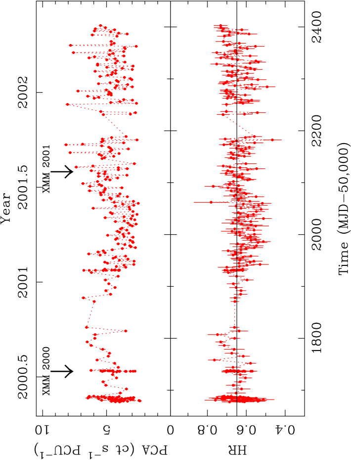
Figure 1: Top panel: the $2-10{\rm\thinspace keV}$ RXTE light curve around the time of the two XMM-Newton observations (during PCA gain epoch 5). Bottom panel: Hardness ratio ($2-4/4-10{\rm\thinspace keV}$). The solid line marks the weighted mean hardness ratio throughout the observing period.

2.1 XMM-Newton observations

XMM-Newton (Jansen et al. 2001) has observed MCG–6-30-15 twice. The first observation was performed during revolution 108 (2000 July 11-12) and the second observation was performed during revolutions 301–303 (2001 July 31 – August 5). In both cases the source was observed on-axis and all instruments were operating nominally. The first results from the 2000 XMM-Newton observation were presented in W01 and the first results from the 2001 XMM-Newton observation were presented in paper I.

During the 2000 observation the pn camera was operated in small window mode, the MOS2 camera in full frame mode and the MOS1 camera in timing mode. During the 2001 observation both the EPIC MOS cameras and the EPIC pn camera were operated in small window mode. For the present analysis only the EPIC data taken in small window mode were used (i.e. only the pn from the 2000 observation, pn and both MOS from the 2001 observation).

The pn small window mode uses a $63\times 64$ pixel window ($\approx 4^{\prime}.3\times 4^{\prime}.4$ on the sky) with the source positioned less than an arcminute from the CCD boundary. The MOS small window mode uses a window of $100\times 100$ pixels ($\approx 1^{\prime}.8\times 1^{\prime}.8$) with the source image approximately centred within the window. The small window modes allow CCD frames to be read out every $5.7$ ms for the pn and $0.3{\rm\thinspace s}$ for the MOS. These short frame times help lessen the effects of photon pile-up which can distort the spectrum of bright sources (Ballet 1999; Lumb 2000). All three EPIC instruments used the medium filter.

2.2 XMM-Newton data reduction

The extraction of science products from the Observation Data Files (ODFs) followed standard procedures using the XMM-Newton Science Analysis System (SAS v5.4.1). The EPIC data were processed using the standard SAS processing chains to produce calibrated event lists. These removed events from the position of known defective pixels, corrected for Charge Transfer Inefficiency (CTI) and applied a gain calibration to produce a photon energy for each event.

Source data were extracted from circular regions of radius $40$^′′from the processed images and background events were extracted from regions in the small window least effected by source photons. These showed the background to be relatively low and stable throughout the observations, with the exception of the final few ks of each revolution where the background rate increased (as the spacecraft approached the radiation belts at perigee). Data from these periods were ignored. The total amount of ‘good’ exposure time selected was $64{\rm\thinspace ks}$ from the pn during the 2000 observation, and for the 2001 observation $315{\rm\thinspace ks}$ and $228{\rm\thinspace ks}$ from the MOS and pn, respectively. (The lower pn exposure is due to the lower ‘live time’ of the pn camera in small-window mode, $\sim 71$ per cent; Strüder et al. 2001).

The ratios of event patterns as a function of energy showed there is negligible pile-up in the pn data but the MOS data suffer slightly from pile-up. This may lead to a slight distortion of the MOS spectra. In order to minimise this effect only photons corresponding to single pixel events (EPIC patterns $0$) were extracted from the MOS cameras. The spectrum of single pixel events should be least affected by pile-up (Molendi & Sembay 2003). For the pn, single pixel (pattern $0$) and double pixel (patterns $1-4$) events were extracted separately for the spectral analysis and fitted simultaneously (the spectrum of single pixel events provides better energy resolution). Response matrices were generated using RMFGEN v1.48.5 and ancillary responses were generated with ARFGEN v.1.54.7. For the 2001 observation source spectra were grouped such that each energy bin contains at least $2,000$ counts for the pn and $400$ counts for the MOS. For the shorter 2000 observation the pn spectrum was grouped to contain at least $500$ counts per energy bin. Background subtracted light curves were extracted from the pn camera in $1000{\rm\thinspace s}$ bins using both single and double pixel events.

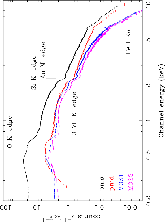
Figure 2: Full-band EPIC spectra. The four sets of data are the pn spectra for single and double events (shown separately) and the MOS1 and MOS2 spectra. For clarity the MOS2 spectrum has been shifted downwards by $20$ per cent. Marked are the positions of the most significant instrumental features (edges due to neutral O, Si and Au) and the positions of the two features expected to be strong in the source spectrum (the O vii edge and Fe K$\alpha$ emission line).

2.3 RXTE observations

MCG–6-30-15 has been regularly monitored by RXTE since 1996. The RXTE Proportional Counter Array (PCA) consists of five collimated Proportional Counter Units (PCUs), sensitive to X-rays in a nominal $2-60{\rm\thinspace keV}$ bandpass and with a total collecting area of $\sim 6250{\rm\thinspace cm}^{2}$. However, due to operational constraints there are usually fewer than five PCUs operated during any given observation. Only data from PCU2 were analysed here as this is the one unit that has been operated consistently throughout the lifetime of the mission. In the following analysis, data from the top (most sensitive) layer of the PCU array were extracted using SAEXTRCT v4.2d. Poor quality data were excluded using standard selection criteria. The PCA background was estimated using the latest version of the ‘combined’ model (Jahoda et al. 2000). Light curves were initially extracted from the STANDARD-2 data with 16 s time resolution. The data were rebinned into quasi-continuous observations lasting typically $1-2{\rm\thinspace ks}$.

3 X-ray history of MCG–6-30-15

Figure 1 shows the RXTE light curve and hardness ratio around the times of the two XMM-Newton observations. From this it is clear that the source displays strong X-ray variability, but most is confined to short term ‘flickering’ rather than longer term trends in the data. A counter example can be seen around MJD 52,000 when there appears to have been a prolonged period of lower flux and variability, during which the spectrum hardened slightly. However, both XMM-Newton observations seem to have caught MCG–6-30-15 in its ‘typical’ state; there are no outstanding secular changes in either flux or hardness ratio to suggest anything other than normal behaviour in the source during the two XMM-Newton observations. The same conclusion is reached when the RXTE monitoring extending back to 1996 are considered. Papadakis et al. (2002) and Uttley, M^cHardy & Papadakis (2002) discuss the RXTE monitoring observations in more detail.

4 Spectral fitting analysis

This section describes the results of the spectral fitting analysis. The raw spectra from the 2001 observation are plotted in Fig. 2. A variety of models, both including and excluding relativistic effects, were fitted to the data. The goal of the analysis was to find the models that can accurately match the data, and test whether models including relativistic effects were preferred. This analysis expands upon the analyses of the same observation presented in paper I, Fabian & Vaughan (2003) and Ballantyne et al. (2003) in that the latest software and calibration were used (as of 2003 May), a wider variety of spectral models was tested, and more information from other observations was used to better constrain the range of the model fits.

4.1 Limits of spectral modelling

The high signal-to-noise of these spectra mean that systematic errors in the detector response model can dominate over the statistical errors (due to photon noise). A brief analysis of some calibration data is discussed in Appendix A. This demonstrated that significant instrumental features should be expected close to the K-edges of O and Si and the M-edge of Au. Elsewhere the spectrum shows no sharp instrumental residuals larger than $\sim 5$ per cent. Therefore in the spectral fitting outlined below, the fitting is primarily carried out over the $3-10{\rm\thinspace keV}$ spectral range that excludes these features. Appendix A also demonstrates that there is a strong discrepancy between the spectral slopes derived from each of the EPIC cameras (see Molendi & Sembay 2003). Therefore the spectral slope of the power-law continuum was always allowed to vary independently between the three EPIC cameras.

With these precautions in place various spectral models were compared to the data as described below. The models were fitted to the four spectra (pn:singles, pn:doubles, MOS1 and MOS2) simultaneously using XSPEC v11.2 (Arnaud 1996). The quoted errors on the derived model parameters correspond to a $90$ per cent confidence level for one interesting parameter (i.e. a $\Delta\chi^{2}=2.71$ criterion), unless otherwise stated, and fit parameters are quoted for the rest frame of the source.

4.2 A first look at the spectrum

The count spectra shown in Fig. 2 give only a poor indication of the true spectrum of the source since they are strongly distorted by the response of the detector. In order to gain some insight into the broad-band shape of the source spectrum, without recourse to model fitting, the EPIC data for MCG–6-30-15 were compared to the spectrum of 3C 273 (see Appendix A). The raw EPIC pn:s data (shown in Fig. 2) were divided by the raw pn:s spectrum for 3C 273. This gave the ratio of the spectra for the two sources. 3C 273 was chosen as it is a bright source and has a relatively simple spectrum in the EPIC band, i.e. a hard power-law plus smooth soft excess modified by Galactic absorption (Page et al. 2003b), and in particular does not contain any strong, sharp spectral features such as lines or edges. Thus the ratio of MCG–6-30-15 to 3C 273 spectra will factor out the broad instrumental response to give a better impression of the true shape of the MCG–6-30-15 spectrum. The top panel of Fig. 3 shows this ratio. The advantage of this plot is that it gives an impression of the MCG–6-30-15 spectrum and is completely independent of spectral fitting. The disadvantages are that it is is in arbitrary units and only gives a very crude representation of the true flux spectrum of MCG–6-30-15 because instead of being distorted by the instrumental response, it is now distorted by the spectrum of 3C 273.

A more accurate, but model-dependent method for obtaining a ‘fluxed’ spectrum of MCG–6-30-15 is to normalise the ratio by a spectral model for 3C 273. This technique is very similar to the method routinely used in optical spectroscopy of normalising the target spectrum using a standard star spectrum to obtain a wavelength-dependent flux calibration. The MCG–6-30-15/3C 273 ratio was multiplied by a spectral model for 3C 273 (defined in flux units). The spectral model comprised a hard power-law plus two blackbodies to model the soft excess, modified by Galactic absorption (see Appendix A and also Page et al. 2003b). This process transformed the raw MCG–6-30-15 count spectrum into a ‘fluxed’ spectrum, without directly fitting the MCG–6-30-15 data. (The accuracy of this procedure does however depend on the accuracy of the 3C 273 spectral modelling.) The fluxed spectrum for MCG–6-30-15 is shown in the bottom panel of Fig. 3.

Note that this procedure is not a formal deconvolution of the spectrum (see Blissett & Cruise 1979; Kahn & Blissett 1980) and so does not correctly take into account the finite detector spectral resolution. Nevertheless, it does provide a simple yet revealing impression of the source spectrum. Specifically, the plot clearly reveals the strongest spectral features in MCG–6-30-15, namely the strong warm absorption concentrated in the $\sim 0.7-2{\rm\thinspace keV}$ region and the iron line peaking at $\approx 6.4{\rm\thinspace keV}$.

Figure 3: EPIC pn:s spectrum of MCG–6-30-15 after normalising by the 3C 273 spectrum. The top panel shows the ratio of counts in the MCG–6-30-15 and 3C 273 spectra. The bottom panel shows the ratio normalised by the spectral model for 3C 273. This reveals the ‘fluxed’ spectrum of MCG–6-30-15 (in units of ${\rm keV}^{2}~{}{\rm s}^{-1}~{}{\rm cm}^{2}~{}{\rm keV}^{-1}$). The ‘fluxed’ spectrum has also been corrected for Galactic absorption. (The sharp feature at $\approx 0.54{\rm\thinspace keV}$ is an artifact caused by the neutral O K-edge in the absorption model being sharper than the instrumental response.)

4.3 Ingredients for a realistic spectral model

4.3.1 Soft X-ray absorption

In the spectral fitting analysis described below the absorption due to neutral gas along the line-of-sight through the Galaxy is accounted for assuming a column density of ${N_{\rm H}}=4.06\times 10^{20}\hbox{${\rm\thinspace cm}^{-2}\,$}$ (derived from $21{\rm\thinspace cm}$ measurements; Elvis, Wilkes & Lockman 1989). Accurately modelling the intrinsic absorption provided a more challenging problem. MCG–6-30-15 is known to possess a complex soft X-ray spectrum, affected by absorption in partially ionised (‘warm’) material (Nandra & Pounds 1992; Reynolds et al. 1995; Otani et al. 1996) and possibly also dust (Reynolds et al. 1997; Lee et al. 2001; Turner et al. 2003a; Ballantyne, Weingartner & Murray 2003). However, the detailed structure of the soft X-ray spectrum, as seen at improved spectral resolution with the grating instruments on board Chandra and XMM-Newton, remains controversial (Branduardi-Raymont 2001; Lee et al. 2001; Sako et al. 2003; Turner et al. 2003a). In the present analysis the complicating effects of the warm absorber were mitigated by concentrating on the spectrum above $3{\rm\thinspace keV}$. However, this will not entirely eliminate the effects of absorption.

In the $3-10{\rm\thinspace keV}$ range absorption by $Z\leq 14$ ions will be limited since their photoionisation threshold energies are less than $3{\rm\thinspace keV}$ for all charge states (the ionisation energy for H-like Si⁺¹³ is $2.67{\rm\thinspace keV}$; Verner & Yakovlev 1995). Similarly, the L-shell of ionised Fe can significantly absorb the spectrum around $1{\rm\thinspace keV}$ due to complexes of absorption lines and edges (e.g. Nicastro, Fiore & Matt 1999; Behar, Sako & Kahn 2001). These transitions all occur below $2.05{\rm\thinspace keV}$ (the ionisation energy of the L-edge in Li-like Fe⁺²³). Thus above $3{\rm\thinspace keV}$ the only opacity from low-$Z$ ions and Fe L will be due to the roll-over of their superposed photoelectric absorption edges. The dominant effect of the warm absorber on the spectrum above $3{\rm\thinspace keV}$ ($\lambda<4.13{\rm\thinspace\AA}$) is thus to impose some subtle downwards curvature on the continuum towards lower energies.

The only significant absorption features occurring directly in the $3-10{\rm\thinspace keV}$ energy range will be due to K-shell transitions in the abundant $Z>14$ elements (S, Ar, Ca, Fe and Ni). Absorption in the $2-5.5{\rm\thinspace keV}$ range could be due to S, Ar and Ca while Fe and Ni may absorb above $6.40{\rm\thinspace keV}$ and $7.47{\rm\thinspace keV}$, respectively. Comparison with the high quality Chandra  HETGS spectrum of the Seyfert 1 galaxy NGC 3783, which shows a very strong warm absorber (Kaspi et al. 2002), suggests that absorption due to S, Ar and Ca is likely to be weak (see the top panel of their figure 1 and also Blustin et al. 2002, Behar et al. 2003). This is confirmed by an analysis of the Chandra HETGS spectrum of MCG–6-30-15 (J. Lee, piv. comm.; see also section 4.5.3).

Turner et al. (2003a) fitted the RGS spectrum from the 2001 XMM-Newton observation using a multi-zone warm absorber model plus absorption by neutral iron (presumably in the form of dust). Although the transmission function of this absorption model recovers above a few ${\rm\thinspace keV}$ it nevertheless predicts the absorption remains significant at higher energies (a $\sim 10$ per cent effect at $3{\rm\thinspace keV}$) due to the combined low-energy edges discussed above. Therefore, to account for the absorption in MCG–6-30-15 this multi-zone absorption model was included in the spectral fitting, with the column densities and ionisation parameters kept fixed at the values derived from fits to the RGS data (these are in any case very poorly constrained by the EPIC data above $3{\rm\thinspace keV}$). The values used are tabulated in Table 1 of Turner et al. (2003a; model 2). The photoelectric edges were included but not the absorption lines. This absorption model therefore accounts for the subtle spectral curvature imposed by the warm absorber. Resonance absorption lines from S, Ar, Ca and Ni are unlikely to contribute significant equivalent width. The possibility of resonance line absorption by Fe is explored separately below.

4.3.2 Iron K-shell absorption

The other noteworthy effects of the warm absorbing material above $3{\rm\thinspace keV}$ are due to the K-shell of iron. Iron in F-like to H-like ions (${\rm Fe}^{+17}-{\rm Fe}^{+25}$) can absorb through K$\alpha$ resonance lines in the $6.4-6.9{\rm\thinspace keV}$ range (Matt 1994; Matt, Fabian & Reynolds 1997) which would be poorly resolved (if at all) in the EPIC spectra. Sako et al. (2003) estimated the resonance lines could produce a total absorption equivalent width of $EW\sim-30{\rm\thinspace eV}$ in MCG–6-30-15 based on an analysis of the Fe L-shell transitions present in the RGS spectrum from the 2000 XMM-Newton observation. This absorption could alter the shape of the observed emission around the Fe K$\alpha$ emission line and was therefore accounted for in the analysis (paper I briefly explored the possible effect of iron resonance absorption).

The other major source of opacity is K-shell photoelectric absorption of photons above $7.1{\rm\thinspace keV}$ (Palmeri et al. 2002). This could affect the continuum estimation on the high energy side of the line, and therefore the apparent line profile, if not properly accounted for (see discussion in e.g. Pounds & Reeves 2002). The edge due to neutral iron is negligible in MCG–6-30-15; the Galactic and intrinsic (dust) neutral absorption gave $\tau\mathrel{\hbox{\hbox to0.0pt{\hbox{\lower 4.0pt\hbox{$\sim$}}\hss}\hbox{$<$}}}0.01$. The warm absorbing material contains Fe in wide a range of charge states, leading to a blurring together of the many K-edges over the $\sim 7.1-9{\rm\thinspace keV}$ range (see Palmeri et al. 2002). In the Turner et al. (2003a) absorption model the total optical depth due to these edges (estimated by comparing the model transmission below the Fe i edge to that at the minimum of the resulting absorption trough) is only $\tau_{\rm max}\sim 0.02$. Using the ionic columns for Fe derived by Sako et al. (2003) gave similar results ($\tau_{\rm max}\sim 0.01$ around the K-edges).

This suggests that while the line-of-sight material does produce iron K-edge absorption, it is rather shallow and spread over the $7-9{\rm\thinspace keV}$ range. The resulting distortion on the transmitted spectrum is far smaller than the statistical errors on the data above $7{\rm\thinspace keV}$ and thus is of little consequence to the spectral fitting. For completeness the absorption due to dust and warm gas in MCG–6-30-15 (as derived by Turner et al. 2003a) was included in the absorption model used below. Furthermore, the $7-10{\rm\thinspace keV}$ EPIC data were searched for additional Fe absorption (see section 4.5.1), such as Fe xxv - xxvi edges which would be undetectable in the lower energy grating spectra (due to the lack of L-shell electrons).

4.3.3 Reflection continuum

Observations of MCG–6-30-15 extending beyond $10{\rm\thinspace keV}$ with Ginga (Pounds et al. 1990; Nandra & Pounds 1994), RXTE (Lee et al. 1998, 1999) and BeppoSAX (Guainazzi et al. 1999; paper I) revealed an upturn in the spectrum and indicated the presence of a reflection continuum. Particularly relevant to the present analysis is that BeppoSAX observed MCG–6-30-15 simultaneously with the 2001 XMM-Newton observation. The data from the PDS instrument provided spectral information extending up to $\sim 100{\rm\thinspace keV}$. Paper I and Ballantyne et al. (2003) presented the results of fitting the BeppoSAX data with reflection models (see in particular section 3 of Ballantyne et al. 2003). These results strongly indicated that the reflection continuum is strong ($R\mathrel{\hbox{\hbox to0.0pt{\hbox{\lower 4.0pt\hbox{$\sim$}}\hss}\hbox{$>$}}}2$).

4.3.4 Narrow iron emission line

As discussed in Section 1, various missions have resolved the broad emission feature spanning the $4-7{\rm\thinspace keV}$ range. In each observation the spectrum can be fitted in terms of a disc line. There could in principle also be a contribution to the reflection spectrum from more distant material ($\gg 100~{}{\thinspace r_{\rm g}}$) which would produce a much narrower, symmetric line. Such lines have been resolved in the spectra of many other Seyfert 1 galaxies (e.g. Yaqoob et al. 2001; Yaqoob, George & Turner 2002; Pounds et al. 2003a; Reeves et al. 2003). The presence of such a narrow ‘core’ could significantly affect model fits to the iron line profile if not correctly accounted for (e.g. Weaver & Reynolds 1998).

In the case of MCG–6-30-15 the variations in the line profile observed by ASCA during a low-flux period (the ‘deep minimum’) suggested the contribution to the line from distant material was small (Iwasawa et al. 1996). The higher resolution Chandra HETGS spectrum (Lee et al. 2002) was able to resolve the peak of the line emission near $6.4{\rm\thinspace keV}$ and confirm that the contribution due to distant material (i.e. an unresolved line ‘core’) is weak ($EW\mathrel{\hbox{\hbox to0.0pt{\hbox{\lower 4.0pt\hbox{$\sim$}}\hss}\hbox{$<$}}}20{\rm\thinspace eV}$). The 2000 XMM-Newton observation of MCG–6-30-15 also showed evidence for narrow line emission (W01; Reynolds et al. 2003). Therefore the possibility of an unresolved iron emission line is allowed in the spectral models considered below.

4.4 Fitting the Fe line core

Figure 4 shows residuals when the EPIC spectra are fitted with a simple model comprising a power-law plus neutral and warm absorption (as discussed in section 4.3.1). The only free parameters were the power-law slope (photon index $\Gamma$) and normalisation. The spectral interval immediately around the Fe K features ($5-8{\rm\thinspace keV}$) was ignored during the fitting, and the model was subsequently interpolated over these energies. The residuals clearly reveal the strong iron K$\alpha$ emission line peaking near $6.4{\rm\thinspace keV}$. The emission line appears asymmetric in this ratio plot, extending down to at least $\sim 5{\rm\thinspace keV}$ (this red wing on the line is far broader and stronger than that expected from the Compton shoulder from cold gas; Matt 2002).

Figure 4: Ratios of EPIC spectra to absorbed power-law model. The model was fitted to the $3-5$ and $8-10{\rm\thinspace keV}$ data. Note the model underestimates the flux on the red side of the line ($\sim 5-6.4{\rm\thinspace keV}$) while the flux is overestimated above $7{\rm\thinspace keV}$. Also note the narrow ‘notch’ at $\approx 6.7{\rm\thinspace keV}$ noticeable in the pn:s spectrum.

As a first step towards modelling the iron features the $5-8{\rm\thinspace keV}$ region was examined in detail. A model was built in terms of a power-law continuum (absorbed as described in section 4.3.1) plus three Gaussian lines. The best-fitting parameters are shown in Table 1. The lines were added to model the resolved line emission (line 1), the unresolved absorption at $\approx 6.7{\rm\thinspace keV}$ (line 2) and the unresolved $6.4{\rm\thinspace keV}$ emission line (line 3). Modelling the line with the single resolved Gaussian emission line provided a reasonable fit, but the inclusion of the unresolved absorption and emission lines significantly improved the quality of the fit. The inclusion of the absorption line was an attempt to account for possible Fe resonance absorption lines (section 4.3.2).

Table 1: Best-fitting parameters for Gaussian models of the iron line core region ($5-8{\rm\thinspace keV}$). ^f indicates the parameter was fixed.

Line	$E({\rm\thinspace keV})$	$\sigma({\rm\thinspace eV})$	$EW({\rm\thinspace eV})$	$\chi^{2}/dof$
1	$6.38\pm 0.02$	$291\pm 33$	$145\pm 15$	$318.5/291$
1	$6.41\pm 0.03$	$312\pm 33$	$167\pm 20$	$300.2/289$
2	$6.73_{-0.04}^{+0.01}$	$10^{f}$	$-11\pm 6$
1	$6.35\pm 0.05$	$405\pm 50$	$148\pm 20$	$263.3/288$
2	$6.74_{-0.09}^{+0.15}$	$10^{f}$	$\geq-8.6$
3	$6.40^{f}$	$10^{f}$	$20\pm 5$

Figure 5 shows the spectrum around the peak of the Fe emission fitted with the three line model (only EPIC pn:s data are shown but all four spectra were included in the fitting). The resolved emission line accounted for the majority of the flux from the core of the Fe emission line, and was significantly resolved with a velocity width $FWHM\approx 4.5\times 10^{4}$ ${\rm\thinspace km}{\rm\thinspace s^{-1}}\,$. Fitting the four EPIC spectra individually with the same model gave consistent results; in each case the emission line was very significantly resolved and the measured widths were consistent with one another.

Figure 5: EPIC pn:s spectrum immediately around the core of the Fe line (crosses). The histograms show the spectral model components, namely a power-law continuum, a broad ($\sigma\approx 410{\rm\thinspace eV}$) Gaussian emission line at $\approx 6.4{\rm\thinspace keV}$, an unresolved emission line at $6.4{\rm\thinspace keV}$ and an unresolved absorption feature at $\approx 6.7{\rm\thinspace keV}$.

The high dispersion velocity width of the emission line core is robust to the details of the underlying continuum fitted over this fairly narrow energy range (it remain significantly resolved after including additional cold gas and/or Fe K edge absorption in the model; see also section 4.5.1). Forcing the entire emission line to be narrow (i.e. unresolved) gave an unacceptable fit ($\Delta\chi^{2}=+266.2$ compared with the resolved line). In addition to $\approx 6.4{\rm\thinspace keV}$ emission there could also be Fe lines at energies $\approx 6.7$ and $\approx 6.9{\rm\thinspace keV}$, corresponding He-like and H-like ions, respectively. The simultaneous presence of iron lines at these three energies (convolved through the EPIC response) could in principle conspire to make the Fe emission mimic a single, resolved line. See Matt et al. (2001) and Bianchi et al. (2003) for an examples where such line blends have been observed in EPIC spectra of Seyferts. Allowing for the presence of three unresolved lines (at energies of $\approx 6.4$, $\approx 6.7$ and $\approx 6.9{\rm\thinspace keV}$) also gave an unacceptable fit. The Fe emission was thus unambiguously resolved by EPIC.

This is of great interest because the resolved line core is considerably broader than those of some other Seyfert 1 galaxies (e.g. Yaqoob et al. 2001; Kaspi et al. 2002; Pounds & Reeves 2002; Page et al. 2003a; Page et al. 2003c) and suggests an origin close to the central SMBH. Neglecting for the time being the contribution of any strongly redshifted component to the line profile, the width of the resolved core can be used to infer the radial distance of the line emitting gas under the assumption that the material is gravitationally bound (and emits at $6.40{\rm\thinspace keV}$ in the rest frame). In this case the rms velocity width of the line ($\sigma$) is determined by its proximity to the SMBH ($r/{\thinspace r_{\rm g}}$) and the geometry according to: $r/{\thinspace r_{\rm g}}\sim(c/\sigma)^{2}/q$ (where $q$ depends on the geometry; Krolik 2001). Assuming randomly oriented circular orbits ($q=3$) places the line emitting material at $r\sim 80{\thinspace r_{\rm g}}$, while assuming a Keplerian disc (inclined at $i=30^{\circ}$; $q=8$) requires the material to be at $r\sim 30{\thinspace r_{\rm g}}$. The resolved line core thus suggests emission from near the central SMBH, necessitating the use of models accounting for the relativistic effects operating in this region.

Fitting this model over the $3-10{\rm\thinspace keV}$ range gave a bad fit ($\chi^{2}=983.1/777~{}dof$) with the emission line energy fixed to $6.4{\rm\thinspace keV}$. Allowing the energy of the broad Gaussian to be free improved the fit ($\chi^{2}=862.1/776~{}dof$) but the Gaussian became extremely broad and redshifted ($E=5.9\pm 0.2{\rm\thinspace keV}$ and $\sigma\mathrel{\hbox{\hbox to0.0pt{\hbox{\lower 4.0pt\hbox{$\sim$}}\hss}\hbox{$>$}}}0.7{\rm\thinspace keV}$). Fitting with two Gaussians to model the broad line (to account for the resolved core and also a highly redshifted component), as well as the narrow $6.4{\rm\thinspace keV}$ emission and $\approx 6.7{\rm\thinspace keV}$ absorption, provided a good fit ($\chi^{2}=730.7/773~{}dof$). The two broad Gaussians had the following parameters: $E_{1}=6.38_{-0.04}^{+0.06}{\rm\thinspace keV}$, $\sigma_{1}=352_{-50}^{+106}{\rm\thinspace eV}$, $EW_{1}\approx 120{\rm\thinspace eV}$ and $E_{2}=4.9_{-1.5}^{+0.2}{\rm\thinspace keV}$, $\sigma_{2}=1.0_{-0.2}^{+0.4}{\rm\thinspace keV}$, $EW_{2}\approx 150{\rm\thinspace eV}$. The energy and width of the second Gaussian further suggests the presence of a highly broadened and redshifted component to the Fe emission. However, such a claim is dependent on the assumed form of the underlying continuum.

4.5 Dependence on the continuum model

The simple absorbed power-law continuum model used above (Fig. 4) clearly overestimated the continuum above $7{\rm\thinspace keV}$ (on the ‘blue’ side of the line). These residuals are a direct result of fitting the continuum with an over-simplistic model, and specifically could be caused by of one of the following: ($a$) additional K-shell absorption by Fe, ($b$) intrinsic curvature in the continuum, ($c$) a continuum curved by excess absorption, or ($d$) excess emission on the red side of the line ($3-5.5{\rm\thinspace keV}$). These last two possibilities would lead to the true continuum slope over the $3-10{\rm\thinspace keV}$ range being underestimated (the fit was driven by the better statistics in the $3-5{\rm\thinspace keV}$ region).

The first three of these alternative possibilities ($a-c$), illustrated in figure 6, are briefly discussed below and found to be unsatisfactory. In the subsequent analysis of sections 4.6 and 4.7 it was assumed that there is excess emission extending from the Fe line to lower energies (i.e. possibility $d$), and this was modelled using relativistic and non-relativistic emission features, respectively.

Figure 6: Schematic of three alternative models that do not include an emission feature on the red side of the iron line. The models comprise a power-law continuum with resolved Gaussian line in addition to: ($a$) additional Fe K-edge absorption, ($b$) a break in the power-law slope at $\approx 6{\rm\thinspace keV}$ and ($c$) enhanced soft X-ray absorption.

4.5.1 Additional iron K absorption?

As discussed in section 4.3.2 the Fe K-shell absorption edges expected based on the grating spectra has been included in the absorption model. It remains possible that there is absorption from additional Fe that was not accounted for in this model.

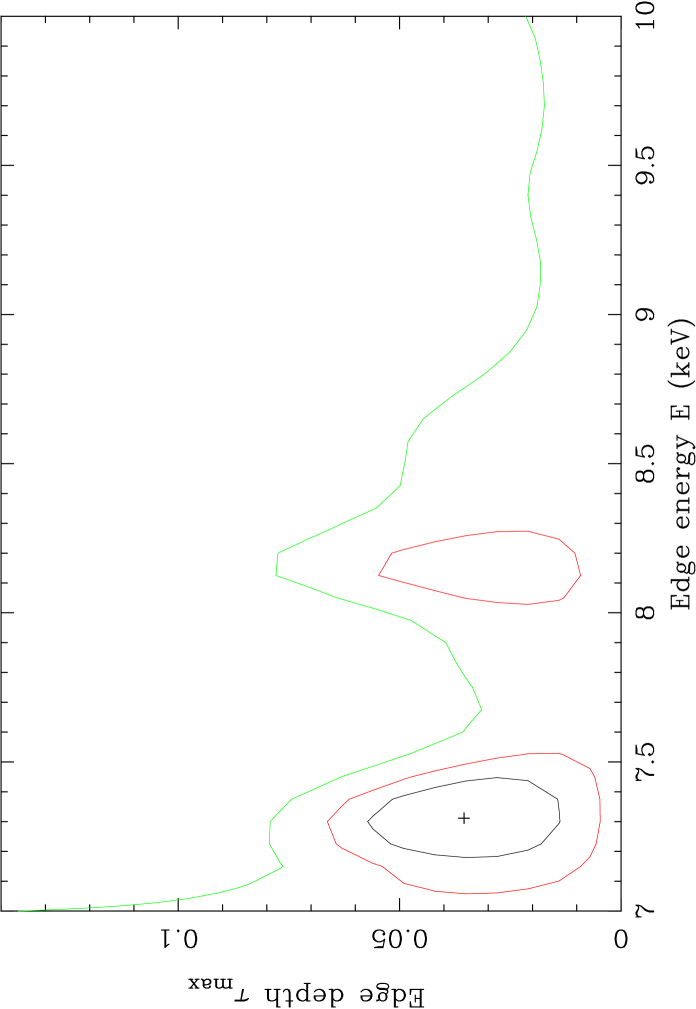
Figure 7: Confidence contours ($68.3,90,99$ per cent limits) on absorption edge parameters when the $7-10{\rm\thinspace keV}$ spectrum was searched for absorption.

The $7-10{\rm\thinspace keV}$ EPIC spectrum was searched for additional absorption by fitting the data over only this limited energy range with a power-law and an absorption edge. Although this model is very simple, over the limited energy range the underlying continuum should not deviate noticeably from a power-law, and with the limited resolution and statistics available at these energies an edge can provide an approximate description of additional Fe absorption.

The data constrain the depth of any such edge to be $\tau<0.06$ ($90$ per cent confidence) over the energies expected for Fe K ($7.11-9.28{\rm\thinspace keV}$). In particular the depth of edge allowed at the energies expected for Fe xxv - xxvi (at the rest-frame velocity of MCG–6-30-15) is $\tau\mathrel{\hbox{\hbox to0.0pt{\hbox{\lower 4.0pt\hbox{$\sim$}}\hss}\hbox{$<$}}}0.03$, ruling out the presence of a large column of such gas (which would have gone undetected in the low energy grating spectra).

The best fitting edge model gave $E=7.31\pm 0.14{\rm\thinspace keV}$ and $\tau=0.036\pm 0.024$. Figure 7 shows the confidence contours for the edge parameters in this ‘sliding edge’ search. Including this edge in the model made virtually no difference to the residuals around the iron line. In particular the apparent asymmetry remained. That said, the best-fitting optical depth should perhaps be treated as an upper limit due to the likely presence of Fe K$\beta$ emission at $E\approx 7.06{\rm\thinspace keV}$, which must accompany the K$\alpha$ emission. Allowing for the possibility of line emission at $E=7.06{\rm\thinspace keV}$ resulted in the edge depth becoming consistent with zero, with a limit of $\tau\leq 0.06$. Including the Fe K edge absorption contained in the model discussed in section 4.3.1 further reduced the depth of any excess Fe absorption.

A caveat is that if a large column of Fe is present with a range of intermediate charge states the resulting absorption will not resemble an edge (Palmeri et al. 2002). However, the low energy grating data do not support the presence of such a large column of ionised Fe in addition to that already included in the model (Lee et al. 2001; Sako et al. 2003; Turner et al. 2003a).

4.5.2 An intrinsically curved $3-10{\rm\thinspace keV}$ continuum?

Ballantyne et al. (2003) and paper I presented analyses of the simultaneous BeppoSAX PDS spectrum of MCG–6-30-15. After allowing for the reflection continuum, the underlying power-law did not show any evidence for intrinsic curvature. In particular, the lower limit on the energy of an exponential cut-off in the continuum was constrained to be $E_{\rm cut}\mathrel{\hbox{\hbox to0.0pt{\hbox{\lower 4.0pt\hbox{$\sim$}}\hss}\hbox{$>$}}}100{\rm\thinspace keV}$. Thus any subtle spectral curvature due to the continuum deviating from a power-law at high energies (as predicted by thermal Comptonisation models) will not affect the $3-10{\rm\thinspace keV}$ bandpass.

As a check for the possible effect of more drastic curvature in the $3-10{\rm\thinspace keV}$ band, the EPIC spectrum was fitted with a broken power-law model, after excluding the region immediately around the Fe K features ($5-8{\rm\thinspace keV}$). This provided a good fit ($\chi_{\nu}^{2}=0.92$). The break in the continuum occurred at $E=4.85_{-0.20}^{+0.86}{\rm\thinspace keV}$ where the slope changed from $\Gamma_{1}=2.00_{-0.04}^{+0.02}$ to $\Gamma_{2}=2.14_{-0.03}^{+0.06}$ above the break energy (the slopes are given based on the pn:s spectrum, similar differences were derived from the other spectra). This form of spectral break, with the spectral slope increasing by $\Delta\Gamma\approx 0.15$ above $5{\rm\thinspace keV}$ is highly unusual and unexpected when compared to other Seyfert 1 spectra. Furthermore, the strong reflection component seen in the BeppoSAX PDS data (section 4.3.3) should lead to a flattening of the spectral slope at higher energies. Indeed, when the broken power-law model was interpolated across the $5-8{\rm\thinspace keV}$ region it predicted a broad iron line extending down to at least $5{\rm\thinspace keV}$ (the energy of the continuum break) but appeared to match poorly the continuum slope at energies above the line (the model was too steep compared to the data above $7{\rm\thinspace keV}$). An intrinsically curved/broken $3-10{\rm\thinspace keV}$ continuum is therefore considered highly unlikely.

4.5.3 Excess soft X-ray absorption?

The warm absorbing gas could perhaps impose curvature on the $3-5.5{\rm\thinspace keV}$ continuum in excess of that already accounted for in the absorption model (section 4.3.1). Significantly higher columns of O or Si ions, for example, would have the effect of increasing the opacity in the high energy tail of the absorption edges occurring at energies $\mathrel{\hbox{\hbox to0.0pt{\hbox{\lower 4.0pt\hbox{$\sim$}}\hss}\hbox{$<$}}}3{\rm\thinspace keV}$. This can be quite effectively modelled by simply allowing the parameters of one of the warm absorbing zones (namely the column density and ionisation parameter) to be free in the fitting. The data were therefore fitted in the $3-10{\rm\thinspace keV}$ range, again excluding Fe K region ($5-8{\rm\thinspace keV}$), using a power-law modified by the absorption model of section 4.3.1 but allowing the parameters of one of the warm absorber zones to vary. The result was that column density of the low ionisation absorber increased to fit better the slight curvature in the $3-5{\rm\thinspace keV}$ band. The fit was good ($\chi_{\nu}^{2}=0.92$) but when the model was interpolated into the Fe K region the residuals again suggested a strongly asymmetric emission feature (as shown in Figure 8). The inclusion of extra absorption below $3{\rm\thinspace keV}$ did therefore not alter the requirement for an asymmetric, red emission feature. However, this model is disfavoured as it severely under-predicted the flux level at lower energies when extrapolated below $3{\rm\thinspace keV}$. Very similar results were obtained after allowing the other (higher ionisation) absorbing zones to vary during the fitting.

Figure 8: Ratio of EPIC pn:s spectrum to an absorbed power-law model. The model was fitted over the ranges $3-5{\rm\thinspace keV}$ and $8-10{\rm\thinspace keV}$ with the absorption model discussed in section 4.3.1 but allowing the parameters of one of the absorbing zones to be free (see section 4.5.3). There is little difference in the pattern of residuals compared with figure 4. In particular there is excess emission on the red side of the line extending down to at least $5{\rm\thinspace keV}$, and again the model slightly overestimates the flux above $7{\rm\thinspace keV}$.

The other possibility, namely that the $3-5.5{\rm\thinspace keV}$ spectrum is significantly affected by S, Ar and/or Ca absorption, was also explored. Absorption by the He- and H-like states of these ions will not affect the spectrum $<2{\rm\thinspace keV}$ (except if they are accompanied by significant columns of M- and/or L-shell ions; Behar & Netzer 2002) and therefore the soft X-ray EPIC and RGS data do not strongly constrain their presence. The upper limit on the optical depth of an absorption edge is $\tau_{\rm max}\mathrel{\hbox{\hbox to0.0pt{\hbox{\lower 4.0pt\hbox{$\sim$}}\hss}\hbox{$<$}}}0.02$ throughout most of this energy range. The only exception is at $\approx 4{\rm\thinspace keV}$ where the addition of a weak edge ($\tau\approx 0.03$) did significantly improve the fit. Thus it remains plausible that some absorption by, for example, highly ionised Argon (e.g. Ar xvii) may weakly contribute in this region. However, this feature must be considered with caution. An examination of the EPIC calibration data for 3C 273 (see Appendix A) revealed similar residuals at the same (observed frame) energy. This feature could thus be due to an instrumental effect at the $\approx 3$ per cent level (possibly due to Ca residuals on the mirror surfaces; F. Haberl priv. comm.). In any event the affect on the derived iron line parameters was negligible.

4.6 Models including strong gravity

The spectral fits detailed above demonstrated that the Fe emission line was significantly resolved, implying emission from near the SMBH. These did not directly address the issue of a highly redshifted component to the line. Furthermore, MCG–6-30-15 shows a strong reflection continuum (section 4.3.3) which needs to be accounted for in the spectral modelling. Therefore, in this section the $3-10{\rm\thinspace keV}$ spectrum is fitted with models accounting for emission from an X-ray illuminated accretion disc extending close to the SMBH (see also W01, paper I and references therein).

The code of Ross & Fabian (1993; see also Ballantyne et al. 2001) was used to compute the spectrum of emission from a photoionised accretion disc. The input parameters for the model were as follows: the photon index ($\Gamma$) and normalisation ($N$) of the incident continuum, the relative strength of the reflection compared to directly observed continuum ($R$) and the ionisation parameter ($\xi=4\pi F_{\mathrm{X}}/n_{\mathrm{H}}$). This model computes the emission (including relevant Fe K$\alpha$ lines), absorption and Compton scattering expected from the disc in thermal and ionisation equilibrium.

To account for Doppler and gravitational effects, the disc emission spectrum was convolved with a relativistic kernel calculated using the Laor (1991) model. The calculation was carried out in the Kerr metric appropriate for the case of a disc about a maximally spinning (‘Kerr’) black hole. The model uses a broken power-law to approximate the radial emissivity (as used in paper I). The parameters of the kernel were as follows: inner and outer radii of the disc ($r_{\rm in},r_{\rm out}$), inclination angle ($i$), and three parameters describing the emissivity profile of the disc, namely the indices ($q_{\rm in},q_{\rm out}$) inside and outside the break radius ($r_{\rm br}$). In addition, narrow Gaussians were included at $\approx 6.4{\rm\thinspace keV}$ to model a weak, unresolved emission line and at $\approx 6.7{\rm\thinspace keV}$ to model the unresolved absorption feature. This emission spectrum (power-law, reflection, narrow emission line) was absorbed using the model discussed in section 4.3.1.

This model gave an excellent fit to the data ($\chi^{2}=652.3/771~{}dof$). The residuals are shown in Fig. 9. The best-fitting parameters corresponded to strong reflection ($R=1.48_{-0.06}^{+0.31}$) from a weakly ionised disc ($\log(\xi)\mathrel{\hbox{\hbox to0.0pt{\hbox{\lower 4.0pt\hbox{$\sim$}}\hss}\hbox{$<$}}}1.4$). The parameters of the blurring kernel defined a relativistic profile from a disc extending in to $r_{\rm in}=1.8\pm 0.1{\thinspace r_{\rm g}}$ with a steep (i.e. very centrally focused) emissivity function within $\approx 3{\thinspace r_{\rm g}}$ and a flatter emissivity without. Specifically, the emissivity parameters were $q_{\rm in}=6.9\pm 0.6$, $q_{\rm out}=3.0\pm 0.1$ and $r_{\rm br}=3.4\pm 0.2{\thinspace r_{\rm g}}$ and the inclination of the disc was $i=33\pm 1^{\circ}$. The narrow emission and absorption lines at $6.4{\rm\thinspace keV}$ and $\approx 6.7{\rm\thinspace keV}$ had equivalent widths of $\approx 10{\rm\thinspace eV}$ and $\approx-10{\rm\thinspace eV}$, respectively. This model is very similar to the best-fitting disc model obtained in paper I from the MOS and BeppoSAX data. The only notable difference between the two models is that the emissivity is more centrally focused in the present model. This is primarily a consequence of including of the EPIC pn data in the fitting, which better defined the red wing of the line, and allowing for narrow Fe K$\alpha$ absorption and emission lines, which subtly altered the appearance of the line profile.

The above model includes emission from well within $6{\thinspace r_{\rm g}}$, the innermost stable, circular orbit (ISCO) for a non-rotating (‘Schwarzschild’) black hole. In order to test whether a Schwarzschild black hole (or specifically $r_{\rm in}\geq 6{\thinspace r_{\rm g}}$) is incompatible with the data the ionised disc model was refitted after convolution with a diskline kernel appropriate for emission around such a black hole (Fabian et al. 1989). The disc was assumed to be weakly ionised ($\log(\xi)=1$), the inner radius was fixed at $r_{\rm in}=6{\thinspace r_{\rm g}}$ in the fitting, and the emissivity was described by an unbroken power-law. This model provided an acceptable fit to the data ($\chi^{2}=698.9/775~{}dof$) albeit substantially worse than the model including emission from within $6{\thinspace r_{\rm g}}$ ($\Delta\chi^{2}=46.6$ between the two models). Thus a model in which the broad iron line and reflection spectrum originate from an accretion disc about a Schwarzschild black hole cannot be ruled out based on the $3-10{\rm\thinspace keV}$ EPIC spectrum. However, the model including emission down to $r_{\rm in}\approx 1.8{\thinspace r_{\rm g}}$ was preferred for two reasons. Firstly it provided a much better fit to the data. Secondly the derived strength of the reflection spectrum for the $r_{\rm in}\approx 1.8{\thinspace r_{\rm g}}$ model ($R\sim 1.4-1.8$) was more compatible with that derived from the independent analysis of the BeppoSAX PDS data ($R\mathrel{\hbox{\hbox to0.0pt{\hbox{\lower 4.0pt\hbox{$\sim$}}\hss}\hbox{$>$}}}2$; section 4.3.3). The best-fitting value for the Schwarzschild model was only $R=0.77\pm 0.04$.

Figure 9: Residuals from fitting the EPIC spectra with a variety of models (for clarity only the EPIC pn:s data are shown). The models comprise an absorbed power-law continuum plus: ($a$) broad Gaussian emission line, ($b$) two broad Gaussians, ($c$) relativistically blurred emission from an accretion disc and ($d$) broad Gaussian and partially covered continuum. Also included is all these models are an unresolved absorption feature at $\approx 6.7{\rm\thinspace keV}$ and an unresolved, neutral iron emission line at $6.4{\rm\thinspace keV}$.

4.7 Models excluding strong gravity

The previous section discussed models in which the spectrum is shaped by strong gravity effects. In this section some trial spectral models are discussed that attempt to explain the spectrum without recourse to strong gravity. In particular, the core of the iron line emission is modelled in terms of a resolved Gaussian and an unresolved emission line, both centred on $6.4{\rm\thinspace keV}$ (see section 4.4). This approximates the distortion on the Fe emission line due to Doppler but not gravitational effects. The asymmetry around the line, in particular the broad excess on the red side, is instead modelled in terms of additional emission components rather than allowing for highly redshifted iron line emission. The possibilities explored are as follows: (i) a blackbody, (ii) a blend of broadened emission lines from elements other than Fe, and (iii) a partially covering absorber.

1. Blackbody emission could provide a broad bump not dissimilar from an extremely broad line. A model comprising a power-law, three Gaussians (resolved and unresolved Fe emission lines and the unresolved absorption feature at $\approx 6.7{\rm\thinspace keV}$) and a blackbody gave a reasonable fit to the data ($\chi^{2}=767.0/775~{}dof$). The blackbody temperature was $kT\approx 1.1{\rm\thinspace keV}$ and it produced a broad excess in flux from $<2{\rm\thinspace keV}$ to $\sim 6{\rm\thinspace keV}$, i.e. on the red side of the line. This model is therefore formally acceptable but the fit is considerably worse than with the relativistic disc models.

2. Along with the K$\alpha$ emission from Fe there may also be K$\alpha$ emission from e.g. S, Ar, Ca or Cr that would also be Doppler broadened. An additional broad Gaussian line was included in the model with a centroid energy in the range $3-5.5{\rm\thinspace keV}$, and a width fixed to be the same as the resolved Fe line. This provided an unacceptable fit ($\chi^{2}=920.6/780~{}dof$). Adding a third broad Gaussian yielded an acceptable fit ($\chi^{2}=809.7/778~{}dof$). The additional lines were centred on $\approx 3.7{\rm\thinspace keV}$ and $\approx 5.0{\rm\thinspace keV}$. The first of these could plausibly be due to Ca xix-xx, but may be caused by a calibration artifact (see section 4.5.3). No strong X-ray line is expected at $\approx 5.0{\rm\thinspace keV}$. The line equivalent widths were $\approx 105{\rm\thinspace keV}$ and $\approx 60{\rm\thinspace keV}$, at least an order of magnitude higher than expected for fluorescence from low-$Z$ elements (e.g. Matt et al. 1997; Ross & Fabian 1993).

3. The presence of partially covered emission (i.e. a patchy absorber; Holt et al. 1980) can cause ‘humps’ in the $2-10{\rm\thinspace keV}$ spectral range. In such model the observed spectrum is the sum of absorbed and unabsorbed emission. A neutral partial covering absorber (with column density, ${N_{\rm H}}$, and covering fraction, $f_{\rm c}$, left as free parameters) was applied to the power-law continuum in the spectral model. Such a model can provide a reasonable fit to the data ($\chi^{2}=745.7/775~{}dof$) with ${N_{\rm H}}\approx 1.4\times 10^{23}\hbox{${\rm\thinspace cm}^{-2}\,$}$ and $f_{\rm c}=0.27\pm 0.03$.

This analysis demonstrated that alternative emission components can reproduce the broad spectral feature observed in the $3-10{\rm\thinspace keV}$ EPIC spectrum. However, these models all give best-fitting $\chi^{2}$ values considerably worse than the relativistic disc model discussed in section 4.6. Possibilities (i) and (ii) are rather ad hoc and physically implausible. A partially covering absorber seems somewhat more reasonable since partial covering has been claimed for other Seyfert galaxies. However, such a model cannot explain the high energy data, in particular, the need for a strong reflection component (section 4.3.3 and see also Reynolds et al. 2003). Furthermore, allowing for partial covering in the model did not eliminate the need for a strongly Doppler broadened iron line.

As a final test of the possible impact of partial covering on fitting the relativistic disc models, the model from section 4.6 was re-fitted including partial covering. The addition of a partially covering absorber to the best-fitting reflection model did not provide a significant improvement to the fit ($\Delta\chi^{2}=2.6$ for two additional free parameters). The derived covering fraction of the absorber was poorly constrained ($0.21\leq f_{\rm c}\leq 1.0$) with a column density ${N_{\rm H}}=5.1_{-0.4}^{+4.9}\times 10^{21}\hbox{${\rm\thinspace cm}^{-2}\,$}$. The inclusion of the partial coverer did not substantially alter the derived values of the relativistic profile parameters (specifically $r_{\rm in}=1.8\pm 0.1{\thinspace r_{\rm g}}$). This analysis suggests that the possible presence of partially covering absorption does not alter the derived parameters for the relativistic emission line. Furthermore, the inclusion of the partial coverer resulted in a lower value for the reflection strength ($R\approx 1.1$), in contradiction with the PDS spectrum ($R\mathrel{\hbox{\hbox to0.0pt{\hbox{\lower 4.0pt\hbox{$\sim$}}\hss}\hbox{$>$}}}2$ see section 4.3.3).

5 Spectral variability

The rapid X-ray variability of MCG–6-30-15 has long been known to show complex energy dependence (e.g. Nandra, Pounds & Stewart 1990; Matsuoka et al. 1990; Lee et al. 1999; Vaughan & Edelson 2001). Vaughan et al. (2003a) used Fourier methods to examine differences between broad energy bands as a function of timescale. In this section the spectral variability is examined in a finer energy scale, at the expense of cruder timescale resolution, in order to probe the details of changes due to specific spectral components. The EPIC data were used over the $0.2-10{\rm\thinspace keV}$ band as the calibration issues discussed above (see also Appendix A) will not affect these analyses.

5.1 Flux-flux analysis

In this section the spectral variability is investigated using ‘flux-flux’ plots. Taylor, Uttley & M^cHardy (2003) used the RXTE data of MCG–6-30-15 to investigate the correlations between the fluxes in different energy ranges. This section parallels their analysis.

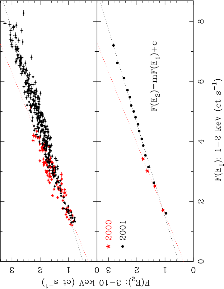
Figure 10: Top panel: correlation diagram comparing EPIC pn count rates in two different energy bands. The points are from $1000{\rm\thinspace s}$ binned light curves. The two observations (2000 and 2001) are marked with different symbols. The dashed line represents the best fitting linear function. Bottom panel: correlation diagram after averaging the data in bins of $20$ points. The points are shown with error bars on both axes, which are of comparable size to the points. The dashed line represents the best fit to the binned data.

Figure 10 shows the count rates in a soft band ($1-2{\rm\thinspace keV}$) against the simultaneous count rates in a hard band ($3-10{\rm\thinspace keV}$) from the $1000{\rm\thinspace s}$ binned EPIC pn light curves. Clearly the two sets of count rates (hereafter fluxes) show a very significant correlation. This is true for both XMM-Newton observations. The data were fitted with a linear model (of the form $F(E_{2})=mF(E_{1})+c$; where $F(E_{1})$ and $F(E_{2})$ represent the fluxes in the two bands) accounting for errors in both axes. This resulted in a formally unacceptable fit (rejection probability $>99.99$ per cent). However, the poorness of the fit is a result of intrinsic scatter in the correlation, rather than any non-linearity. This intrinsic scatter in the relation between different energy ranges is a manifestation of both the difference in shape of the power spectral density (PSD) function and low coherence between variations in different energy bands (Vaughan et al. 2003a). Therefore, to overcome this the data were then binned such that each bin contains $20$ points and errors were calculated in the usual fashion (equation 4.14 of Bevington & Robinson 1992). The binned data, which reveal the average flux-flux relation, provided a reasonable fit to a linear function (rejection probabilities of $33$ and $89$ per cent for the 2000 and 2001 datasets, respectively).

As concluded by Taylor et al. (2003) the tight linearity of the flux-flux correlation (at least over the relatively short time scales probed by each XMM-Newton observation) strongly indicates that the flux variations are dominated by changes in the normalisation of a spectral component with constant softness ratio $m$ (i.e. the gradient of the flux-flux correlation). In addition there must be an additional spectral component that varies little and contributes more in the $3-10{\rm\thinspace keV}$ band than the $1-2{\rm\thinspace keV}$ band and therefore produces the positive constant offset $c$. In other words the flux in each band is the sum of a variable component and a constant component:

$$F(E)=N_{\rm V}V(E)+N_{\rm C}C(E)$$ (1)

(where $N_{\rm V}$ and $N_{\rm C}$ are the normalisations of the variable and constant spectra $V(E)$ and $C(E)$ respectively) . The fact that the relation between $F(E_{1})$ and $F(E_{2})$ is linear means that the gradient gives $m=V(E_{2})/V(E_{1})$ and the offset gives $c=C(E_{2})-mC(E_{1})$. As can be seen from the figure the relation changed between the 2000 and the 2001 observations; these changes in slope and offset imply the shape of the two spectral components differed slightly between the two XMM-Newton observations. The flux-correlated changes in the spectrum are caused by changes in the relative contributions of these two spectral components. This ‘two component’ interpretation of the X-ray spectral variability of Seyfert 1s has been discussed by e.g. Matsuoka et al. (1990); Nandra (1991); M^cHardy et al. (1998); Shih et al. (2002); Fabian & Vaughan (2003).

5.1.1 Decomposing the spectrum

As discussed in Fabian & Vaughan (2003), the ‘difference spectrum’ can be used to determine the shape of the variable component of the spectrum, $V(E)$ (see section 5.2). The offset of the flux-flux plot, $c$, gives a measure of the strength of the constant component in the spectrum and so by measuring the offset as a function of energy, $c(E)$ it is possible to estimate the spectrum of the constant component $C(E)$ (see section 4.3 of Taylor et al. 2003). Figure 11 shows the spectrum of the constant component in MCG–6-30-15 deduced by measuring the offset $c(E)$ of the flux-flux relations. Binned flux-flux plots were constructed by comparing the light curves in each energy band to the $1.0-1.5{\rm\thinspace keV}$ band ($F(E_{1})$). In each case the constant offset was measured from the best fitting linear model and normalised to the average flux in the energy band under examination. This yielded an estimate of the fractional contribution to the spectrum from non-varying components.

The spectrum of the constant component shown in figure 11 reveals that the constant component is soft below $\sim 1{\rm\thinspace keV}$ and hard at higher energies. The largest fractional contribution from the constant component occurs in the iron K band, where it contributes $\sim 40$ per cent of the total flux. There are two assumptions implicit in this analysis. The first is that the variable component has a constant spectral shape $V(E)$ when averaged as a function of flux (which is implied by the linearity of the flux-flux relations). The second assumption is that there is a negligible constant component in the $1.0-1.5{\rm\thinspace keV}$ band (which was used as the comparison), i.e. $C(E_{1})=0$. If the $1.0-1.5{\rm\thinspace keV}$ emission does contain a non-zero constant component ($C(E_{1})>0$) then the absolute scale of the inferred spectrum would increase but its spectral form will be approximately the same. The maximum possible amount of constant emission in the $1.0-1.5{\rm\thinspace keV}$ band is given by the minimum flux in that band (i.e. $0\leq C(E_{1})\leq\min[F(E_{1})]$), therefore this can be used to place an absolute limit on the strength of the constant component: $c(E)\leq C(E)\leq\{c(E)+m(E)\min[F(E_{1})]\}$. This upper limit is also indicated in figure 11. It should be noted that the constant component $C(E)$ must be affected by the soft X-ray absorption. The lack of features associated with absorption in figure 11 (in particular the lack of a spectral jump at $\sim 0.7{\rm\thinspace keV}$) demonstrates that the constant component is affected by absorption exactly as is the total spectrum (hence the absorption was factored out by normalising the spectrum $C(E)$ by the total spectrum). This spectrum can be identified with the Reflection-Dominated Component (RDC) of Fabian & Vaughan (2003) and is henceforth referred to as the RDC.

Figure 11: Fractional contribution to the spectrum of the constant component ($C(E)/\overline{F(E)}$ deduced from the linear flux-flux relation). The errors are $1\sigma$ confidence limits obtained from the linear fit to the flux-flux data. If the constant component contributes a non-zero fraction in the $1.0-1.5{\rm\thinspace keV}$ range the contributions at all energies will increase but the spectral shape will remain the same. The arrows indicate the absolute upper limits on the fraction of constant emission (see text).

5.2 Flux-resolved spectra

A more conventional way to examine how the spectrum of the source evolves with flux is to extract energy spectra from different flux ‘slices.’ This was done for the 2001 XMM-Newton data by dividing the pn data into ten flux intervals such that the total number of photons collected from the source in each flux interval was comparable ($\sim 5\times 10^{5}$). The highest and lowest flux slices differ by a factor of $3$ in count rate and all ten are marked on the light curve in Figure 12. The ten spectra extracted from each flux slice were then binned in an identical fashion. There were clear, systematic spectral changes between the ten flux intervals, these are illustrated in two different ways in figures 13 and 14. Figure 13 shows the ten spectra as ratios to a ($\Gamma=2$) power-law model (modified only by Galactic absorption). This illustrates the softening of the $2-10{\rm\thinspace keV}$ spectrum as the source gets brighter. In addition the strength of the iron line relative to the continuum gets weaker as the source brightens (i.e. the equivalent width decreases with increasing continuum luminosity) meaning that the iron line becomes a lower contrast feature at high fluxes.

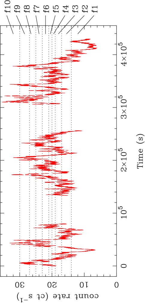
Figure 12: $0.2-10{\rm\thinspace keV}$ EPIC pn light curve of the 2001 observation. The light curve has been divided into ten count rate intervals marked $f1-f10$.

Figure 14 shows nine of the ten spectra as a ratio to the highest flux spectrum ($f10$). This again shows the spectrum became harder (in the $2-10{\rm\thinspace keV}$ range) and the iron line became relatively stronger as the source became fainter. It is also interesting to note that at energies below $\sim 2{\rm\thinspace keV}$ the spectrum becomes softer as the source becomes fainter, contrary to the trend at higher energies. In addition, there is no strong feature in the spectral ratios at $\sim 0.7{\rm\thinspace keV}$, indicating that the fractional strength of the $\sim 0.7{\rm\thinspace keV}$ spectral jump remains constant with flux. This is consistent with the jump being due to absorption with a constant optical depth.

Figure 13: EPIC pn spectra from each of the count rate slices (shown in figure 12) compared to a $\Gamma=2$ power-law model (modified by Galactic absorption). The data have been shifted upwards to aid clarity. It can be seen that as the flux decreases from $f10$ to $f1$ the overall spectrum becomes harder (above $2{\rm\thinspace keV}$) and the strength of the iron feature decreases (relative to the continuum model).

Figure 14: EPIC pn spectra from the count rate slices shown as a ratio to the highest count rate spectrum ($f10$). Similar to figure 13 the spectra can be seen to become harder and show relatively stronger iron features as the count rate decreases.

These average changes in the detailed spectral shape as a function of flux can be explained using the simple two-component model discussed above. The inferred constant emission comprises a soft excess below $\sim 1{\rm\thinspace keV}$, a harder tail above $\sim 2{\rm\thinspace keV}$, and a strong iron line. One would expect the total (variable$+$constant) spectrum to change exactly as observed: as the total flux decreases the contribution from the constant component, relative to the variable component, increases. Therefore, at low fluxes, the spectrum will become softer below $\sim 1{\rm\thinspace keV}$, harder above $\sim 2{\rm\thinspace keV}$, and display a more prominent iron line.

5.2.1 Average EPIC difference spectrum

The five highest flux spectra were combined, as were the five lowest flux spectra, to produce two spectra representing the source during flux intervals above and below the mean (hereafter ‘high’ and ‘low’ fluxes). Subtracting the low flux spectrum from the high flux spectrum will remove the contribution from the constant component. As discussed in Fabian & Vaughan (2003), under the assumption that the total spectrum can be accurately described (on average) by the superposition of two emission components, one variable and one not (both modified by absorption), the difference spectrum will give the spectrum of only the variable component (modified by absorption): $F_{hi}(E)-F_{lo}(E)=(N_{\rm V,hi}-N_{\rm V,lo})V(E)$ (where $V(E)$ includes absorption).

Figure 15 shows the EPIC pn difference spectrum (compared to a power-law model fitted in the $3-10{\rm\thinspace keV}$ range) from the 2001 observation. A power-law (modified only by Galactic absorption) gave an excellent fit to the $3-10{\rm\thinspace keV}$ data ($\chi^{2}=28.1/60~{}dof$) and yielded a photon index of $\Gamma=2.20\pm 0.05$. Extrapolating this power-law down to lower energies reveals the signature of strong absorption, although the exact amount depends on the assumed shape of the underlying continuum (as illustrated by the upper and lower datasets shown in the figure). It also be noted that if the variable spectral component steepens at low energies (i.e. contains a soft excess) the inferred absorption profile at lower energies could be systematically underestimated even further (see section 6 of Turner et al. 2003a). Leaving aside these uncertainties on the inferred spectrum at lower energies, it remains true that above $3{\rm\thinspace keV}$ the average spectrum of the varying component $V(E)$ can be described accurately as a single power-law ($\Gamma\approx 2.2$). In particular it should be noted that the difference spectrum (unlike the spectrum of the constant component described above) does not possess any obvious features in the iron K region. The upper limit on the flux of the line core (section 4.4) present in the difference spectrum is a factor $\sim 20$ lower than that present in the time averaged spectrum.

A further investigation of the flux-resolved spectra revealed that the difference spectrum is consistent with a power-law at all flux levels. Nine difference spectra were calculated by subtracting the lowest flux spectrum ($f1$) from each of the nine higher flux spectra ($f2-f10$). These nine difference spectra were fitted over the $3-10{\rm\thinspace keV}$ range with an absorbed power-law model. In all nine cases the simple power-law model was found to provide a good fit to the data ($\chi_{\nu}^{2}\approx 1.0$), with no evidence for strong systematic residuals around the Fe K band. The limit on the depth of possible Fe edges in the $7.1-8{\rm\thinspace keV}$ region was $\tau\mathrel{\hbox{\hbox to0.0pt{\hbox{\lower 4.0pt\hbox{$\sim$}}\hss}\hbox{$<$}}}0.07$, consistent with the limits obtained in section 4.5.1. In the discussion below this variable component to the spectrum will be referred to as the variable Power-law Component (PLC; Fabian & Vaughan 2003).

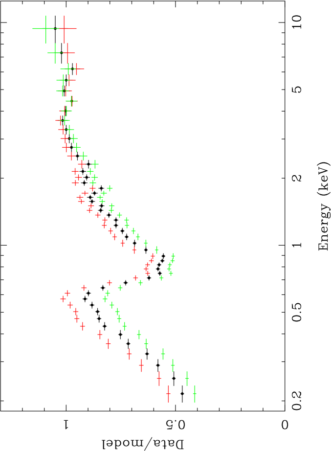
Figure 15: EPIC pn difference spectra produced by subtracting the low flux spectrum from the high flux spectrum. The difference spectrum is shown as a ratio to a power-law (modified by Galactic absorption) fitted across the $3-10{\rm\thinspace keV}$ range. The data/model ratio calculated using the best fitting power-law slope is shown in black (circles). Above and below this lie the ratios calculated assuming the $90$ per cent lower and upper limits on the slope of the $3-10{\rm\thinspace keV}$ power-law. The data were rebinned for clarity.

5.3 rms spectra

The root mean squared (rms) spectrum measures the variability amplitude as a function of energy and can in principle reveal which spectral components are associated with the strongest variability (see Edelson et al. 2002 and Vaughan et al. 2003b). Figure 16 shows two rms spectra calculated from the 2001 XMM-Newton observation of MCG–6-30-15, clearly showing in both cases a strong dependence of the variability amplitude on energy.

The two rms spectra show the variability amplitude on different timescales. The upper spectrum shows the fractional rms amplitude integrated over the entire observation in the standard fashion (eqn. 1 of Edelson et al. 2002) using $1000{\rm\thinspace s}$ binned light curves. As the variability is dominated by long timescale changes (Uttley et al. 2002; Vaughan et al. 2003a) this therefore reveals the energy dependence of variations occurring on timescales comparable to the length of the observation ($\sim 100{\rm\thinspace ks}$). The lower spectrum shows the fractional rms of the point-to-point deviation (i.e. the rms difference between adjacent time bins, as defined by eqn. 3 of Edelson et al. 2002). This therefore only measures fluctuations between neighbouring time bins and so probes the energy dependence of the variability on short timescales comparable to the bin size ($\sim 1{\rm\thinspace ks}$). The errors were calculated as in eqn. 2 of Edelson et al. (2002), but as discussed in their appendix should be considered only as approximations since they strictly assume the light curves are drawn from independent Gaussian processes. Matsumoto et al. (2003) previously used the longest ASCA observation of MCG–6-30-15 to obtain rms spectra on different timescales.

As is clear from the figures the rms spectra show broad peak at $\sim 1{\rm\thinspace keV}$ and a localised depression around the energy of the iron K emission line, strongly suggesting a suppression of the variability due to the presence of the emission line (see also Inoue & Matsumoto 2001). The exact energy dependence of the variability amplitude differs between the two timescales (evident from the ratio of the two rms spectra), as should be expected if the shape of the PSD is a function of energy (Vaughan et al. 2003a).

Figure 16: Top panel: fractional rms variability amplitudes as a function of energy on two different timescales. The upper data represent the amplitude integrated over the entire (2001) observation while the lower data represent the rms deviation between neighbouring points (point-to-point rms) and therefore samples only short timescale variability ($\sim 1000{\rm\thinspace s}$). The errors were calculated as described in the text. The dashed line indicates the energy of the (neutral) Fe K$\alpha$ line ($6.40{\rm\thinspace keV}$). The histogram shows the ‘two component’ model rms spectrum. Bottom panel: The ratio of the two rms spectra, showing how the energy dependence of the variability amplitude changes with variability timescale.

5.3.1 Modelling the rms spectrum

In the previous sections is was shown how the spectral variability is consistent with a model comprising a variable component $V(E)$ (the PLC; see Figure 15) and a constant component $C(E)$ (the RDC; see Figure 11). Given these empirically derived spectral components it is possible to construct a model for the rms spectrum shown in Figure 16 (see also Inoue & Matsumoto 2001).

It is assumed that the spectrum is given by equation 1 where both $V(E)$ and $C(E)$ include absorption effects. The (normalised) rms spectrum can be expressed as:

$$F_{\rm var}(E)=\frac{\sigma[F(E)]}{\overline{F(E)}}=\frac{\sqrt{\sigma[N_{\rm V}V(E)]^{2}+\sigma[N_{\rm C}C(E)]^{2}}}{\overline{N_{\rm V}}V(E)+\overline{N_{\rm C}}C(E)}$$ (2)

where $\sigma[F(E)]$ and $\overline{F(E)}$ represent the absolute rms amplitude and time-average of the spectrum over the observation, respectively. (Likewise for the two spectral components $V(E)$ and $C(E)$.) In terms of the model being discussed it is assumed that $C(E)$ is not variable and so $\sigma[N_{\rm C}C(E)]=0$. Therefore:

$$F_{\rm var}(E)=\frac{\sigma[N_{\rm V}V(E)]}{\overline{N_{\rm V}}V(E)+\overline{N_{\rm C}}C(E)}$$

$$=\frac{\sigma[N_{\rm V}]}{\overline{N_{\rm V}}}(1-C(E)/\overline{F(E)})$$ (3)

and the term $C(E)/\overline{F(E)}$ is the fractional contribution of the constant component shown in Figure 11.

The above analysis assumes that the variable component changes only in normalisation and not in shape (i.e. $\sigma[N_{\rm V}V(E)]/\overline{N_{\rm V}V(E)}=\sigma[N_{\rm V}]/\overline{N_{\rm V}}$), but is independent of the actual form of the spectrum $V(E)$. The linearity of the flux-flux relations implies the variable component has a constant softness ratio with flux, and therefore its spectrum $V(E)$ is independent of flux, validating this assumption. The first term on the right-hand side of equation 3 is thus simply a normalisation. Implicit in this analysis is the assumption that the absorption function is not time-variable. If the absorption function did vary this would introduce another term to the rms spectral model (Inoue & Matsumoto 2001), but such a term is not required by the data and thus it was assumed that the absorption did not vary.

The histogram in Figure 16 shows the resulting rms spectral model when the constant component derived in section 5.1 (Figure 11) is used. This very simple model clearly reproduces (to within $\sim 1$ per cent in $F_{\rm var}$) the energy dependence of the variability amplitude on these timescales. The peak at $\sim 1{\rm\thinspace keV}$ is a result of the constant component $C(E)$ being weakest at $\sim 1{\rm\thinspace keV}$ and the suppression at $\sim 6.4{\rm\thinspace keV}$ results from the strong iron line present in the constant component. The short timescale rms spectrum has a subtly different shape and thus it not so well reproduced using this simple model. However, it is known that at high frequencies the variability in different energy bands shows different PSD shapes and incoherent variability. Thus the short timescale rms spectrum will be affected by these additional effects, although their physical origin is not clear. This could perhaps be explained if the RDC (or perhaps the warm absorber) varies on short timescales but these changes are ‘washed out’ over longer timescales.

5.3.2 A low-flux rms spectrum

The shape of the rms spectrum is clearly a function of timescale, as expected given the energy-dependent PSD (Vaughan et al. 2003a). It also shows subtle changes with time when the rms spectrum of each revolution of XMM-Newton data are compared (an rms spectrum for the first revolution was shown in paper I). These may be caused by subtle changes in the RDC spectrum. As the relative strength of the RDC should be highest when the overall source flux is low, the low flux intervals of the light curve are the most promising to search for changes in the RDC.

The rms analysis described above was repeated using only the last $45{\rm\thinspace ks}$ of data from rev 0303. During this time interval the source flux was rather low and in fact reached its minimum for the observation (Fig. 12). The rms spectra from this interval are shown in Fig. 17. The low-flux rms spectrum, particularly on the longer timescale, shows a similar overall shape to the rms spectrum from the entire observation (upper data from Figs.  16 and  17). Interestingly the prediction of the two component model discussed above does not match these data so well. In particular the model predicts either too little rms around the iron line or too much in the soft X-ray band. This could be indicating that at low fluxes some variation in the shape/strength of the RDC were detected (see also Reynolds et al. 2003). However, this could also result from a random effect caused by the energy-dependent PSD (Vaughan et al. 2003a,b). More observations at very low flux levels could confirm whether the RDC shows rapid variability.

Figure 17: The rms spectra, as shown in Fig. 16, including only the low flux interval towards the end of the observation.

5.4 Time-resolved spectra

For completeness the spectrum was examined in consecutive $10{\rm\thinspace ks}$ time slices. Fig. 18 shows the spectra extracted from each of these time slices. Clearly the strength of the iron line (relative to the continuum model) changes throughout the light curve. However, the only obvious, visible change is that described above; as the overall X-ray flux decreases the iron line becomes more prominent because it varies less than the continuum. For example, the spectrum for segment 303:l, which has one of the lowest fluxes, also has the most prominent line.

It is possible that there are short-lived spectral features that would be ‘washed out’ in the time-averaged spectrum. Turner, Kraemer & Reeves (2003b) discuss the possible existence of transient, redshifted iron lines. However, given that $32$ independent spectra were examined here, the likelihood of an apparently significant feature appearing purely by chance is quite high. For example, the probability of detecting a feature, considered detected at $99.7$ per cent confidence in one individual spectrum, in one of the $32$ spectra is $\sim 0.1$ (using $P_{N}\approx 1-(1-P_{1})^{N}$). By the same argument only features found at $>3.5\sigma$ significance in any individual spectrum should be considered as significant detections from the entire dataset (i.e. probability of false detection $P_{N}\mathrel{\hbox{\hbox to0.0pt{\hbox{\lower 4.0pt\hbox{$\sim$}}\hss}\hbox{$<$}}}0.01$). There are no clear examples of strong, sharp features in these data except for the obvious iron line. The analyses of Fabian & Vaughan (2003) and Ballantyne et al. (2003) demonstrated that these time-resolved spectra can be fitted using relatively simple reflection models. In addition, there were no sharp features seen in the rms spectra (section 5.3) that would indicate a preferred energy for transient features.

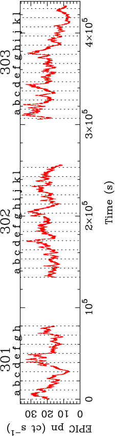
Figure 18: Top panel: EPIC pn $0.2-10{\rm\thinspace keV}$ light curve spanning all three XMM-Newton revolutions with $10{\rm\thinspace ks}$ time intervals labelled. Bottom panels: EPIC pn spectra extracted from the $10{\rm\thinspace ks}$ time intervals, shown as a ratio to a simple power-law model. The expected energy of the iron line ($6.4{\rm\thinspace keV}$) is marked with a dotted line.

5.5 Principal Component Analysis

The method of Principal Component Analysis (PCA) was used to try and isolate independently varying components present in the time-resolved spectra discussed above. PCA is a powerful statistical tool used widely in the social sciences where it is often known as factor analysis. In practice PCA gives the eigenvalues and eigenvectors of the correlation matrix of the data. The data can be thought of as an $m\times n$ matrix comprising $m$ observations of the $n$ variables, in which case the correlation matrix would be a symmetric $n\times n$ matrix.

The eigenvectors can be thought of as defining a new coordinate system, in the $n$-dimensional parameter space, which best describes the variance in the data. The first principal component, or PC1 (the eigenvector with the highest eigenvalue), marks the direction through the parameter space with the largest variance. The next Principal Component (PC2) marks the direction with the second largest amount of variance. The motivation behind PCA is to extract the (hopefully few) dominant correlations from a complex dataset. Francis & Wills (1999) provides a brief introduction to PCA as applied to quasar spectra, while Whitney (1983) and Deeming (1964) illustrate more general applications of PCA in astronomy.

If the variance in the spectra is caused by only a few independently varying spectral components then PCA should reveal them in its eigenvectors. The application of PCA to spectral variability of AGN was first discussed by Mittaz, Penston & Snijders (1990). The first few Principal Components (those representing most of the variance in the data) should reveal the shape of the relevant spectral components. The weaker Principal Components might be expected to be dominated by the photon noise in the spectra (which should be uncorrelated between each of the $n$ energy bins in the $m$ spectra and so should not distort the shape of the first Principal Components).

This method was used on the $m=32$ time-resolved spectra over the $3-10{\rm\thinspace keV}$ range (binned such that they each spectrum contained the same $n=21$ energy bins). The spectra were unfolded using a $\Gamma=2$ power-law model to convert them from counts to flux units (in $EF(E)$ form). In the absence of sharp features in either the source spectrum or the detector response this should provide a reasonable estimate of the ‘fluxed’ data. The first three Principal Components are shown in Figure 19 along with the mean and rms spectra derived from the same data.

As can be clearly seen, PC1 has a relatively flat spectrum and describes the vast majority of the variance in the data ($96$ per cent). The first Principal Component can therefore be identified with the variable PLC discussed above. All the remaining Principal Components each describe less than $1$ per cent of the variance and most likely represent only the photon noise in the data. Thus the PCA confirms the above analyses and suggests the spectral variations in MCG–6-30-15 are a result of a single, varying continuum component (the PLC). Nearly identical results were found when the ranked data was used to produce the correlation matrix (which then represented the matrix of rank-order correlation coefficients).

Figure 19: Results of Principal Component Analysis (PCA). The top panel shows the mean spectrum (converted into $EF(E)$ flux units). The next two panels show the rms and fractional rms of the data (after subtracting the contribution from photon noise). The bottom three panels show the spectra of the first three Principal Components and their contribution to the total variance of the data ($P_{\rm var}$). The solid line marks the zero level; points that lie on the same side of the zero line (all positive or all negative) are correlated with one another while points that lie on different sides of the zero line (differing signs) are anti-correlated.

6 The 2001-2000 difference spectrum

Figure 20 shows the difference spectrum produced by subtracting the $3-10{\rm\thinspace keV}$ EPIC pn:s spectrum taken in 2000 from the spectrum taken in 2001. A power-law provided a good fit ($\chi^{2}=51.7/62~{}dof$) with $\Gamma=2.18\pm 0.09$ (compare with the results of section 5.2.1). The only significant residuals appeared as an excess at $\approx 6.6{\rm\thinspace keV}$. Including a narrow Gaussian improved the fit ($\chi^{2}=44.1/60~{}dof$), with a best-fitting energy $E=6.63\pm 0.12{\rm\thinspace keV}$. Including an absorption edge in the model did not significantly improve the upon this fit. Figure 21 shows the ratio of the two spectra, confirming that the two spectra differ around $E\approx 6.65{\rm\thinspace keV}$.

An unresolved emission feature in the difference and ratio spectra could be due to a change in either the flux of the broad Fe emission line or the depth of the Fe K$\alpha$ absorption. In order to produce an apparent emission feature in the first case only the blue wing of the emission line must be stronger in the 2001 observation. In the second case the optical depth of the absorption must be deeper in the 2000 observation. An examination of the two spectra individually suggested the latter is more likely. A close examination of changes in the RGS spectrum between the two observations would clarify this issue.

Figure 20: Difference spectrum produced by subtracting the 2000 data from the 2001 data. Only the EPIC pn:s spectrum is shown. The only significant residual (compared to the simple power-law continuum model) is an unresolved ‘emission’ feature at $E=6.65\pm 0.05{\rm\thinspace keV}$.

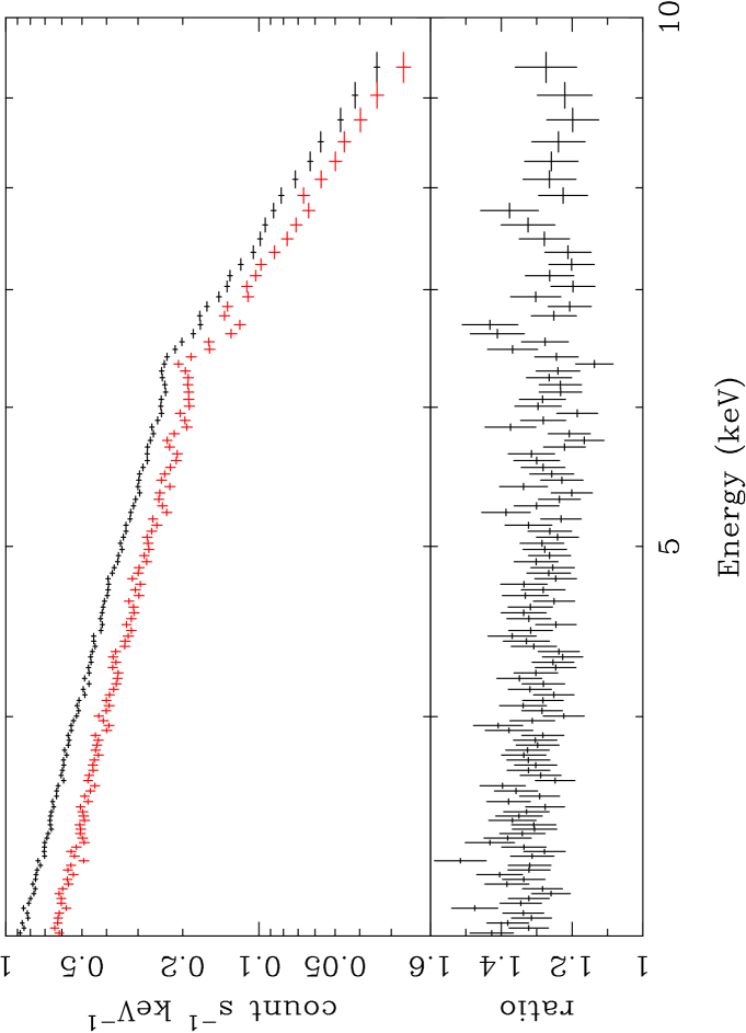
Figure 21: Ratio of the EPIC pn:s spectral from the 2001 (upper data) and 2000 (lower) observations. The top panel shows the raw spectra, the bottom panel shows their ratio. This again shows the unresolved ‘emission’ feature at $E\approx 6.65{\rm\thinspace keV}$.

7 Review of XMM-Newton results

In this section the main results obtained from the long XMM-Newton observation of MCG–6-30-15 are summarised prior to the discussion in the following section.

• The two XMM-Newton observations (taken in 2000 and 2001) sampled fairly typical ‘states’ of the source. The former observation sampled a period of lower flux than the latter. However, the long-term RXTE monitoring shows this can be attributed to short-term variability and does not imply a systematic difference between the states of the source during the two observations (section 3).

• The high energy spectrum obtained from BeppoSAX shows a strong Compton-reflection signature (paper I; Ballantyne et al. 2003), as did the earlier XMM-Newton/RXTE observation (W01; Reynolds et al. 2003). There was no evidence for a low energy cut-off or roll-over in the continuum out to $\sim 100{\rm\thinspace keV}$.

• The RGS spectrum shows complex absorption by O vii, O viii and Fe i as well as a range of other ions (Sako et al. 2003; Turner et al. 2003a). The opacity is concentrated mainly below $\sim 3{\rm\thinspace keV}$ but still has an important effect on the $3-10{\rm\thinspace keV}$ spectrum (section 4.3.1). See also Lee et al. (2001).

• The fluorescent iron line is strong and broad (section 4.4). The bulk of the line flux is resolved with EPIC. The emission peak concentrated around $6.4{\rm\thinspace keV}$ is resolved with a width $FWHM\approx 4.5\times 10^{4}$ ${\rm\thinspace km}{\rm\thinspace s^{-1}}\,$, strongly indicating an origin within $\mathrel{\hbox{\hbox to0.0pt{\hbox{\lower 4.0pt\hbox{$\sim$}}\hss}\hbox{$<$}}}100{\thinspace r_{\rm g}}$. There is also a significant, asymmetric extension to lower energies that indicates strong gravitational redshifts. In addition there is a weak, intrinsically narrow core to the line emission (sections 4.3.4 and 4.4; see also Lee et al. 2002).

• The best-fitting model for the $3-10{\rm\thinspace keV}$ EPIC spectrum explained the iron emission as from the surface of a relativistic accretion disc. The strong reflection explains the strength of both the iron line and the Compton reflection continuum. The best fitting model includes emission down to $\approx 1.8{\thinspace r_{\rm g}}$ (section 4.6; W01; paper I).

• The variations in X-ray luminosity show many striking similarities with those seen in GBHCs such as Cygnus X-1 (Vaughan et al. 2003a). In particular, the Power Spectral Density (PSD) function is similar to that expected by simply re-scaling the high/soft state PSD of Cyg X-1. The continuum variations are energy dependent and show the PSD is a function of energy and that the hard variations are delayed with respect to the soft variations. Similar results have been found in other Seyfert 1s (NGC 7469, Papadakis, Nandra & Kazanas 2001; NGC 4051, M^cHardy et al. 2003).

• Previous observations with ASCA (Iwasawa et al. 1996, 1999; Shih et al. 2003) and RXTE (Lee et al. 2001; Vaughan & Edelson 2001) showed the photon index of the $2-10{\rm\thinspace keV}$ continuum to be correlated with its flux. The XMM-Newton observations confirm this and demonstrate the trend is reversed below $\sim 1{\rm\thinspace keV}$, where the spectrum hardens with increasing flux (section 5.2). The average variability amplitude is highest in the range $\sim 1-2{\rm\thinspace keV}$, and is lowest at energies around the iron line (section 5.3).

• The variable spectrum can be decomposed into two components, a variable Power-law component (PLC; section 5.2.1) and a relatively constant Reflection Dominated Component (RDC; section 5.1). The spectral variability (at least on timescales $\sim 10{\rm\thinspace ks}$) can be explained almost entirely by variations in the relative strength of these two components, caused solely by changes in the normalisation of the PLC (section 5.3; see also Shih et al. 2003 and Fabian & Vaughan 2003). An analysis of the flux-flux plots (section 5.1; see also Taylor et al. 2003) and the difference spectra (section 5.2.1) shows the slope of the PLC remains approximately constant with flux.

• The EPIC spectrum indicates there is resonance absorption by ionised Fe at $\approx 6.7{\rm\thinspace keV}$ (sections 4.3.2 and 4.4). This was predicted based on the presence of soft X-ray warm absorption (Matt 1994; Sako et al. 2003) and has been observed in at least one other high quality EPIC spectrum (NGC 3783; Reeves et al. 2003). This resonance absorption appeared to vary between the two XMM-Newton observations (section 6).

8 Discussion

8.1 Fitting the iron line in MCG–6-30-15

The broad iron line in MCG–6-30-15 has been unambiguously resolved using XMM-Newton/EPIC (W01; paper I; this paper), confirming the previous results from ASCA (Tanaka et al. 1995; Iwasawa 1996), BeppoSAX (Guainazzi et al. 1999) and Chandra (Lee et al. 2002). However, deriving reliable line profile parameters is a considerable challenge even with the exceptionally high quality XMM-Newton$+$BeppoSAX data. From the whole of the $320{\rm\thinspace ks}$ observation the EPIC cameras collected about $6\times 10^{3}$ counts from the core of the line, peaking at $6.4{\rm\thinspace keV}$, and about three times as many from the broad red tail of the line emission.

The foremost problem is that there are no regions of the X-ray spectrum unaffected by either the warm absorption (see section 4.3.1) or the broad emission components. Thus it is not possible to determine the underlying continuum without simultaneously constraining the other spectral components. Often used, simple techniques for determining the continuum by e.g. fitting a power-law over the $3-5{\rm\thinspace keV}$ and $7-10{\rm\thinspace keV}$ data (Nandra et al. 1997), will give a only crude first approximation of the continuum. In a source such as MCG–6-30-15, which possesses a strong warm absorber, the absorption will cause the spectrum to curve even above $\sim 3{\rm\thinspace keV}$ (see section 4.3.1 and Fig. 3). In the present paper this effect was dealt with by including an absorption model derived from fits to the RGS data (section 4.3.1) and also allowing for additional absorption when fitting the EPIC data (section 4.5).

In addition to the distortion imposed on the continuum the other effect of warm absorption that has a significant impact on iron line studies is resonant line absorption at $\approx 6.4-6.9{\rm\thinspace keV}$ (section 4.3.2). The EPIC data indicate the presence of such absorption; allowing for the Fe resonance absorption had a subtle but significant effect on the best-fitting emission line models (see section 4.4). In particular, the line profile is slightly broader and bluer after accounting for the line absorption.

Photoelectric absorption by Fe at energies $\sim 7.1-9.3{\rm\thinspace keV}$ could, in principle, also be caused by the warm absorbing gas and further confuse the continuum estimation (see e.g. Pounds & Reeves 2002). However, in the case of MCG–6-30-15 this is not a significant effect. The total opacity due to the Fe K edges, as predicted based on fits to the soft X-ray RGS data, is negligible (section 4.3.2), and spectral analysis of the EPIC data confirm this by ruling out the presence of deep Fe edges (section 4.5.1). The same is not true of all Seyfert 1s galaxies. The columns of Fe ions derived using RGS data by Blustin et al. (2002) for NGC 3783, and by Sako et al. (2001) for IRAS 13349+2438 predict strong K edges with a total optical depth $\tau_{\rm max}\sim 0.05$ (see also Reeves et al. 2003).

Further complications include the presence of the reflection continuum (section 4.3.3) and possible weak, narrow components to the line emission (section 4.3.4). The approach used in the present paper was an attempt not to ‘unambiguously isolate’ the iron line but to model it after allowing for these complicating factors. In order to limit the range of models and free parameters, constraints obtained from other instruments (such as the RGS and BeppoSAX spectra) were used where possible. The result of this spectral fitting confirms the previous analyses in W01 and paper I: The best-fitting emission model comprises a power-law continuum plus strong reflection from a weakly ionised, relativistic accretion disc (section 4.6). This model requires the disc emission to be centrally concentrated and extend in to $\sim 2{\thinspace r_{\rm g}}$. Attempts to ‘explain away’ the red wing of the line using enhanced absorption or broken continua (section 4.5) did not substantially alter the main results. Additionally, alternative emission components such as iron line blends did not fit the data (section 4.4) while emission from soft X-ray lines or blackbodies led to physically implausible results (section 4.7).

The only non-standard model that could fit the data with plausible parameters was the partial covering model (section 4.7). However, as shown also by Reynolds et al. (2003), this model is strongly at odds with the higher energy data. Thus, a partially covered continuum does not provide a satisfactory explanation of the X-ray spectrum of MCG–6-30-15. However, it is possible that the source does contains some partially covered emission in addition to the disc reflection. Fitting the data with a relativistic disc and also allowing for partial covering suggested the possible impact of the partial covering is minimal (section 4.7).

8.2 Spectral variability of MCG–6-30-15

The spectral variability of the source can be explained in terms of a two-component model (section 5.1; see also M^cHardy et al. 1998; Shih et al. 2002; Taylor et al. 2003; Fabian & Vaughan 2003). This is the simplest model consistent with the flux-flux analysis.

In this model the two spectral components are a power-law component (PLC) and a reflection dominated component (RDC) which carries most of the iron line flux. Both of these emission spectra are viewed through the warm absorbing gas. Flux variations are caused primarily by changes in the normalisation of the PLC, with the RDC remaining relatively constant. Such a model explains many aspects of the spectral variability including the linearity of the flux-flux plots (section 5.1), the rms spectrum (section 5.3), the correlation between $2-10{\rm\thinspace keV}$ spectral slope and flux (section 5.2) and the lack of strong iron line variations (Reynolds 2000; Vaughan & Edelson 2001; paper I). The relative constancy of the RDC causes variations above $\sim 2{\rm\thinspace keV}$ (and particularly around the iron line) to be suppressed, and also variations below $\sim 1{\rm\thinspace keV}$ are increasingly suppressed (section 5.3). Fabian & Vaughan (2003) previously applied this model to direct fitting of the time-resolved EPIC spectra, where it gave a quite reasonable description of the time varying spectrum.

The spectrum of the PLC was uncovered using the hi–low difference spectrum (Fabian & Vaughan; section 5.2) and the spectrum of the RDC was obtained by isolating the constant offset of the flux-flux plots (Taylor et al. 2003; section 5.1). This latter technique revealed the spectrum of the constant RDC independent of any spectral fitting, simply by analysing the light curves using flux-flux plots. The result clearly revealed a spectral form strongly suggestive of reflection, with a prominent iron line (as suggested by Fabian & Vaughan 2003). The RDC also shows a ‘soft excess’ below $\sim 1{\rm\thinspace keV}$ which could also be emission from the reflecting disc if it is weakly ionised. The model derived from fitting the $3-10{\rm\thinspace keV}$ EPIC spectra is in rough qualitative agreement with the RDC spectrum obtained independently (see Fig. 22). Thus the model derived from spectral fitting (section 4) is in broad agreement with the model invoked to explain the spectral variability (section 5).

Figure 22: Fractional contribution to the spectrum of the constant component deduced as in Fig. 11. The dotted curve shows the prediction based on the model derived from fitting the EPIC spectra in the $3-10{\rm\thinspace keV}$ range only. Clearly the model has qualitatively the same shape, although the details do not match, particularly at lower energies. However, given that the model was derived without using the spectral data below $3{\rm\thinspace keV}$, and there is an intrinsic uncertainty in the normalisation of the RDC (section 5.1), the agreement is rather interesting.

8.2.1 Variability constraints on complex absorption models

The warm absorption spectrum does not appear to vary substantially (specifically, the optical depths of the absorption features remain approximately constant). For example, ratio plots of ‘high’ and ‘low’ spectral (section 5.2) show smooth profiles over the deepest absorption features, as does the rms spectrum (section 5.3). This result is consistent with the studies of the deep warm absorber in NGC 3783 using Chandra (Netzer et al. 2003) and XMM-Newton (Behar et al. 2003) which showed the X-ray absorption remained unchanged despite large changes in source luminosity.

Furthermore, the spectral variability constrained the possible effect of warm or partial absorption on the iron line. Neither of the two spectral components isolated through spectral variability analysis resemble the absorbed part of the continuum in the partial covering model. The depth of any line-of-sight Fe K edge was constrained by the difference spectrum analysis (section 5.2) to be $\tau\mathrel{\hbox{\hbox to0.0pt{\hbox{\lower 4.0pt\hbox{$\sim$}}\hss}\hbox{$<$}}}0.02$ at $7.1{\rm\thinspace keV}$ to $\tau\mathrel{\hbox{\hbox to0.0pt{\hbox{\lower 4.0pt\hbox{$\sim$}}\hss}\hbox{$<$}}}0.07$ at $8.0{\rm\thinspace keV}$. Fitting the partial covering model to the various difference spectra gave constraints comparable to those based on the time-averaged spectrum (section 4.7). As discussed above the effect of including such additional absorption (either warm or partial) on the derived iron line parameters was negligible.

Alternative models for the spectral variability of MCG–6-30-15 in which the variations are caused primarily by changes in the warm absorber (Nandra et al. 1990; Inoue & Matsumoto 2003) are in stark contrast with the data. This model predicts a power-law flux-flux relation (since the flux is given by $f(E,t)=S(E)\exp(-\tau(E,t))$, where $S(E)$ is the underlying the emission spectrum and $\tau(E,t)$ is the time-variable absorption optical depth). Such a model would also predict strong features in the rms spectrum corresponding to the deepest edges in the absorption spectrum (paper I). Both of these were ruled out.

8.3 Outstanding issues with the disc model

8.3.1 Lack of iron line variations

Although the model outlined above explains many aspects of the EPIC spectrum and its variability, there are some serious outstanding problems. The most significant of these is how the RDC flux, including the iron line, remains so steady in the presence of large changes in the flux of the PLC. In standard accretion disc/reflection models the reflection spectrum (including iron line) is fundamentally driven by the PLC luminosity. Thus, since the RDC is thought to originate close to the SMBH (and the source of the PLC) the fluxes of the two components should be tightly coupled. The lack of correlations between the iron line and continuum is a long-standing issue (Iwasawa et al. 1996, 1999; Lee et al. 2000; Reynolds 2000; Vaughan & Edelson 2001). These XMM-Newton observations demonstrate more clearly than before that not just the line but the bulk of the reflected emission (the RDC) shows little short-timescale variability. The physics responsible for the reduced variability of the RDC is unclear.

During the 2001 XMM-Newton the total EPIC count rate from the iron line was $\sim 0.1$ ct s^-1, with $\sim 0.02$ ct s^-1 coming from the resolved, quasi-Gaussian core on the line and the rest coming from the broad, red wing. As a result of this low count rate, compounded by the modelling difficulties, it is difficult to place firm limits on weak and/or extremely rapid (faster than $\sim 10^{4}{\rm\thinspace s}$) line variations. Intriguingly, Reynolds et al. (2003) claim that variations in the line/RDC become apparent only when the source flux is very low (see also Iwasawa et al. 1996).

One possibility is the progressive ionisation of disc surface, as discussed by e.g. Reynolds (2000), Nayakshin & Kazanas (2002) and Ballantyne & Ross (2002). In this scenario an increase in the ionising luminosity leads to little change in the flux of the line because more of the Fe ions in the surface layers of the disc become fully-stripped of electrons. Under some circumstances this model can explain the lack of iron line variations (Reynolds 2000). However, the spectral fitting analysis (section 4) suggests the emitting region of the disc is only weakly ionised. Time-resolved spectral fitting of the XMM-Newton data using an ionised disc model (Ballantyne et al. 2003) showed that ionisation effects could not reproduce the constancy of the RDC. A second reflector that was intrinsically constant was also required. Thus, ionisation effects alone are insufficient to explain the lack of iron line variations.

One intriguing alternative possibility is that gravitational light bending, which may be strong if the disc extends to $\sim 2{\thinspace r_{\rm g}}$, is (partially) responsible (Fabian & Vaughan 2003). See Miniutti & Fabian (2003) for a detailed discussion of this model. Such a model may naturally explain the enhanced reflection strength ($R\mathrel{\hbox{\hbox to0.0pt{\hbox{\lower 4.0pt\hbox{$\sim$}}\hss}\hbox{$>$}}}2$; section 4.3.3) and iron line.

An interesting and related question is: how does the PLC retain its spectral shape whilst undergoing factors of $\sim 5$ changes in luminosity? Both direct time-resolved spectral fitting (e.g. Fabian & Vaughan 2003) and flux-flux analyses (section 5.1; Taylor et al. 2003) show the slope of the PLC to stay remarkably constant. Similar results have been seen in ultrasoft Seyfert galaxies (e.g. Vaughan et al. 2002) where the primary power-law slope stays constant despite large amplitude luminosity variations. This poses an interesting challenge to models of the origin of the primary X-rays which typically predict some luminosity-correlated variation in slope (e.g. Zdziarski et al. 2003). The observations are suggestive of some kind of ‘Compton thermostat’ (Haardt, Marachi & Ghisellini 1994; Pietrini & Krolik 1995). Alternatively, if the apparent variations in the PLC flux are due to geometrical effects near the SMBH, the PLC might be expected to vary achromatically (Miniutti et al. 2003).

8.3.2 Inner edge of the disc

The intricacies of modelling the complex spectrum of MCG–6-30-15 have made it difficult to tap the potential of the iron line profile for probing the region of strong gravity around the SMBH. An often asked question is: how far in towards the SMBH does the disc extend? The answer to such a question may reveal the spin of the SMBH (e.g. Stella 1990; Martocchia et al. 2002). The strength/shape of the red wing of the line is determined by the emissivity of the innermost disc and so are the primary diagnostics of the position of the disc’s inner boundary. The problem is that the very broad, low-contrast tail to the line is difficult to discern from the spectral curvature caused by the warm absorber (see Fig. 3). Thus it is not possible to unambiguously determine the inner disc edge (unless the transmission of the warm absorber is known to very high accuracy). For example, the method of Bromley, Miller & Pariv (1998) works by identifying the ‘minimum energy’ of the red wing of the redshifted line emission. However, no such energy can be identified without detailed, simultaneous modelling of the absorption and the reflection continuum.

This does not mean that all is lost. The method of fitting the reflection emission while simultaneously fitting/constraining the absorbed continuum did require emission in to $\sim 2{\thinspace r_{\rm g}}$ (W01; paper I; section 4.6). Importantly, this result was robust to various possible effects that might bias the continuum determination (sections 4.5 and 4.7). This is strong but not conclusive evidence that the SMBH is spinning. An alternative approach to fitting the red wing of the line (perhaps isolating it through variability if the red wing shows variations on very short timescales not yet probed) would bolster the determination of its profile.

The second and more fundamental objection is that some emission is possible from within $6{\thinspace r_{\rm g}}$ even if the SMBH is not spinning (see Reynolds & Begelman 1997; Young, Ross & Fabian 1998; Krolik & Hawley 2002; Merloni & Fabian 2003). Further refinement of the theory combined with a further increase in observational sensitivity should be able to settle this issue (see Young & Reynolds 2000; Yaqoob 2001).

8.3.3 Why do only some Seyferts show broad lines?

Recent, high-quality Chandra and XMM-Newton observations of bright Seyfert galaxies seem to have produced a mixed bag of iron lines. Examples of strong, narrow lines have been found in NGC 3783 (Kaspi et al. 2002; Reeves et al. 2003), NGC 5548 (Yaqoob et al. 2001; Pounds et al. 2003a), NGC 4151 (Schurch et al. 2003), and NGC 3227 (Reeves 2003). Examples of highly broadened iron lines have been seen in MCG–5-23-16 (Dewangan et al. 2003), NGC 3516 (Turner et al. 2003c), IRAS 18325–5926 (Iwasawa et al. in prep.), Q 0056–363 (Porquet & Reeves 2003), IRAS 13349+2438 (Longinotti et al. 2003) and Mrk 766 (Mason et al. 2003; Pounds et al. 2003b). The line in MCG–6-30-15 is the broadest of the known broad lines. There are some objects for which the line profile is in dispute (e.g. Mrk 205 and Mrk 509, see Pounds et al. 2001; Reeves et al. 2001; Page et al. 2003c). Even more confusing is the possible detection of rapidly variable yet narrow iron lines in Mrk 841 (Petrucci et al. 2002) and NGC 7314 (Yaqoob et al. 2003). Recent studies of GBHCs have also revealed relativistically broadened iron lines in a few cases (Miller et al. 2003; Miller et al. 2002).

This raises two obvious, related questions. The first is: why do some Seyferts show strong, broad lines while others show only narrow lines (with any highly broadened component being weak or absent)? The second question is: how can some Seyferts not have broad lines? The high luminosities of AGN in general argues that there must be a large amount of mass flowing deep into the potential well of the SMBH. Furthermore, the rapid X-ray variability argues that the X-ray source is spatially compact and probably also located close to the SMBH. There should be a substantial amount of relatively cool accreting matter in the region of strong gravity around the SMBH, close to the primary X-ray source. These are the only two ingredients thought necessary to produce a broad iron line (Fabian et al. 1989; Reynolds & Nowak 2003). The absence of broad lines in many Seyfert 1s is therefore quite puzzling and requires that either there simply is not enough cool matter extending close to the SMBH to produce the line or that the line photons are somehow lost (absorbed/scattered) on their way out of the inner regions. See also Reeves et al. (2003) for a discussion of this problem.

It is important to note that there could be some observational biases present. By their very nature highly broadened lines are difficult to isolate (as discussed above). The broad line in MCG–6-30-15 is perhaps the most clear example in part due to the strength of the reflection spectrum. The high level of reflection ($R\mathrel{\hbox{\hbox to0.0pt{\hbox{\lower 4.0pt\hbox{$\sim$}}\hss}\hbox{$>$}}}2$) means that the equivalent width of the broad line is rather high ($EW\sim 400{\rm\thinspace eV}$). Other Seyfert galaxies with more typical reflection strengths ($R\sim 1$) would be expected to have comparably weaker broad lines ($EW\sim 150{\rm\thinspace eV}$; George & Fabian 1991). Even with the high throughput of the EPIC cameras on-board XMM-Newton, a typical length observation ($\sim 40{\rm\thinspace ks}$) of a bright Seyfert 1 might not clearly reveal a redshifted line with $EW\sim 150{\rm\thinspace eV}$. This is especially true if the continuum is absorbed. Thus, most observations of Seyfert 1s are unlikely to show broad lines; the lack of an obvious broad line in the spectrum does not rule out its existence. These observations can constrain the strength of highly broadened lines (e.g. upper limits on the equivalent width of a Laor profile) and so place useful limits on the line emission. This will help address the question of whether broad lines are a rare or common occurrence.

8.4 Iron resonance absorption

The fits to the iron line allowing for resonant absorption suggest the presence of an additional absorber whose dominant effect is Fe xxv He$\alpha$ absorption at $\approx 6.7{\rm\thinspace keV}$. This absorption appears to have varied between the 2000 and 2001 XMM-Newton observations (section 6). Such an absorption system can be modelled (using the CLOUDY grids of Turner et al. 2003a) with a high column (${N_{\rm H}}\mathrel{\hbox{\hbox to0.0pt{\hbox{\lower 4.0pt\hbox{$\sim$}}\hss}\hbox{$>$}}}10^{22}\hbox{${\rm\thinspace cm}^{-2}\,$}$) and high ionisation ($\log(\xi)\approx 3$) warm absorber. This is similar to the results obtained for another bright Seyfert 1, NGC 3783 (Reeves et al. 2003) except that this very high ionisation absorption does not significantly affect the low energy spectrum. Similar features may have been observed in other Seyferts (NGC 3516, Nandra et al. 1999; IRAS 13349-2438, Longinotti et al. 2003).

Another approach is to estimate the column density using just the equivalent width ($EW\sim 10{\rm\thinspace eV}$) of the absorption line and the assumption that He-like Fe is the dominant ion in the absorbing material. Using the oscillator strength of the Fe xxv He$\alpha$ line from Nahar & Pradhan (1999) the column density can be estimated assuming the line is unsaturated (linear part of the ‘curve of growth’; Spitzer 1978). This gives $N_{\rm Fe^{+24}}\sim 10^{17}\hbox{${\rm\thinspace cm}^{-2}\,$}$. If the line is saturated the column density will be higher. The predicted depth of the corresponding Fe xxv absorption edge (at $8.83{\rm\thinspace keV}$) is $\tau\sim 0.05$, consistent with the limits obtained from the data (section 4.5.1). Assuming solar abundances and that half all the Fe ions are in the He-like state this column corresponds to ${N_{\rm H}}\mathrel{\hbox{\hbox to0.0pt{\hbox{\lower 4.0pt\hbox{$\sim$}}\hss}\hbox{$>$}}}4\times 10^{21}\hbox{${\rm\thinspace cm}^{-2}\,$}$. This compares reasonably to the estimate derived from the CLOUDY model, but should really be considered only a lower limit on the total column density since it does not account for other (lower oscillator strength) lines, possible line saturation or emission line filling.

8.5 The Future

The long XMM-Newton observation of MCG–6-30-15 has yielded a vast amount of detailed information (on absorption and emission spectra, variability timescales and delays and spectral changes). Only by making full use of the long and simultaneous observations (CCD and grating X-ray spectra) possible with XMM-Newton (and simultaneous BeppoSAX observations) could all of these be achieved. Comparable observations have been performed/planned for a small sample of other Seyferts (for example: NGC 3783, Behar et al. 2003; Reeves et al. 2003) which will shed light on the detailed X-ray properties of Seyferts in general. Complimentary to these are the Chandra long-looks that have been particularly enlightening for warm absorber studies (e.g. Kaspi et al. 2002). Such observations also demonstrate the limits of present instrumentation. For example, without higher resolution, high S/N spectroscopy it is difficult to realise the diagnostic potential of the $6.4-6.9{\rm\thinspace keV}$ iron resonance absorption lines.

The presence of such a large column of highly ionised iron makes MCG–6-30-15 a good choice for high resolution Fe-band spectroscopy with the XRS on-board Astro-E 2. This has the capability (with resolution $\Delta E\sim 7{\rm\thinspace eV}$ and good throughput) to measure the depths and velocity shifts of some of the individual resonance lines. Indeed, the combination of the high resolution XRS spectrum of the iron absorption/emission, the high energy HXD spectrum which will constrain the continuum and reflection, and the high throughput XIS spectrum should provide the next major advance towards making full use of the information contained in the X-ray spectra of Seyferts.

Aside from future missions, the present data indicate the most interesting observations are often made when the source is very faint. The spectral analysis presented above showed that when MCG–6-30-15 is faintest, the iron line is strongest relative to the continuum, making it a much higher contrast feature. The rare observations that show apparent changes in iron line properties tend to occur during periods of unusually low flux (Iwasawa et al. 1996; Reynolds et al. 2003). Observations of NGC 4051 during its prolonged ‘low states’ have revealed other interesting phenomena, such as the warm absorbing gas in emission (Uttley et al. 2003). Thus it would seem that XMM-Newton and Chandra observations of bright Seyfert 1s, taken during periods of unusually low activity, may prove particularly revealing.

9 Conclusions

The long XMM-Newton observation of MCG–6-30-15 has confirmed the existence of a highly broadened iron line. The main results of the present investigation are as follows:

1. It is not yet possible, given the present state of knowledge of the detailed properties of the warm absorber, to unambiguously dis-entangle the red wing of the line from the absorbed continuum.

2. Nevertheless, the best-fitting model requires the reflection/line emitting region to extend inwards to $\sim 2{\thinspace r_{\rm g}}$. This result was robust to various possible biases in the continuum determination.

3. Alternative models for the spectral region around the iron line, not allowing for the effects of strong gravity, gave unsatisfactory results.

4. The spectral variability of MCG–6-30-15, including the correlation between $2-10{\rm\thinspace keV}$ slope and flux and the reduced variability of the iron line, has been explained using a two-component model.

5. The relative constancy of the reflection dominated component (RDC), in the presence of large variations in the power-law component (PLC), is the primary cause of the spectral variations. The reasons for the lack of RDC variations are unclear. A model invoking gravitational light bending near the SMBH can qualitatively explain the suppressed variations, the relative strength of the RDC and the small inner disc radius.

Appendix A Analysis of EPIC calibration data

This section describes an analysis of EPIC data taken from observations of 3C 273 ($z=0.158$). This source is bright, point-like (compared to the EPIC PSF) and shows a relatively simple energy spectrum in the EPIC bandpass (i.e. approximately power-law with no sharp spectral features), making it useful for assessing the accuracy of the EPIC spectral calibration.

Five observations of 3C 273 were analysed. These observations were taken primarily for performance verification and calibration purposes and the observation details are given in Table LABEL:tab:cal. During all five observations the source was positioned on-axis and all three EPIC cameras used small window mode and medium filter (i.e. the same instrumental set-up as the MCG–6-30-15 observations). The only exception is the first half of the rev. $277$ observation during which the MOS cameras used the thin filter (data from this part of the observation were ignored). This later observation was used by Molendi & Sembay (2003) to assess the EPIC calibration.

Table 2: Details of observations used for calibration purposes.

		Observation	Observing time	Duration
Source	Revolution	ID	(UT)	(s)
3C 273	094	0126700301	2000 Jun 13 23:39:53–2000 Jun 14 20:05:49	73556
3C 273	095	0126700601	2000 Jun 15 12:58:18–21:35:30	31032
3C 273	095	0126700701	2000 Jun 15 23:32:02–2000 Jun 16 09:37:48	36346
3C 273	096	0126700801	2000 Jun 17 23:24:14–2000 Jun 18 19:50:15	73561
3C 273	277	0136550101	2001 Jun 13 07:14:26–2001 Jun 14 08:10:31	89765

Figure 23: Confidence contours from fitting the 3C 273 EPIC spectra (from revs. $0094-0096$) over the $3-10{\rm\thinspace keV}$ range with a power-law model.

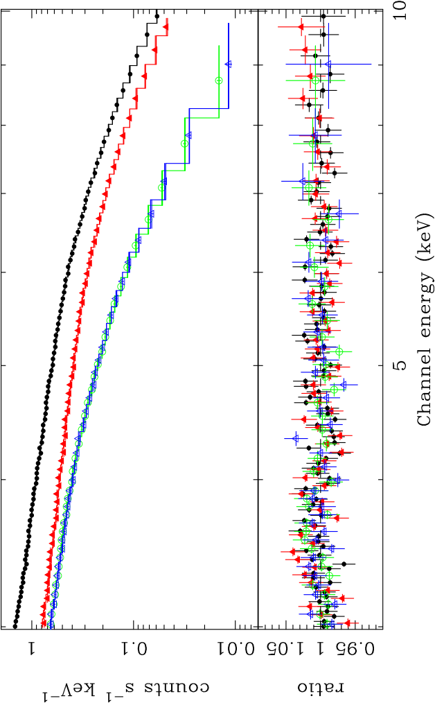
Figure 24: $3-10{\rm\thinspace keV}$ EPIC spectra of 3C 273 from revs. $094-096$. The four sets of data are for pn single (filled circles) and double events (filled triangles), MOS1 (hollow circles) and MOS2 (hollow triangles) The spectra were fitted with a model comprising a power-law and a Gaussian emission line.

Source and background spectra were extracted exactly as for the MCG–6-30-15 observation. Only single pixel event were used from the MOS to reduce the effect of pile-up in this bright source (see Molendi & Sembay 2003). The grouped spectra were then fitted in the $3-10{\rm\thinspace keV}$ range with a simple power-law modified by Galactic absorption (${N_{\rm H}}=1.79\times 10^{20}\hbox{${\rm\thinspace cm}^{-2}\,$}$; Dickey & Lockman 1990). The power-law indices and normalisations were left independent for each camera. In all five observations the spectra from each camera showed weak but positive residuals at $5-6{\rm\thinspace keV}$, suggesting the presence of iron line emission. Previous studies of 3C 273 (e.g. Turner et al. 1990; Grandi et al. 1997; Reeves 2003) also suggested the presence of weak iron emission. A Gaussian was therefore included in the model at $6.4{\rm\thinspace keV}$ (in the source frame) to account for iron emission (with equivalent width $EW\sim 20{\rm\thinspace eV}$). This simple model provided an acceptable fit to all five sets of spectra (i.e. $\chi_{\nu}^{2}<1.0$) and showed that the four sets of spectra taken during rev. $094-096$ were very similar (i.e. the source showed no spectral variability during this period). Therefore the data from the four observations spanning these revolutions were combined to produce a high signal-to-noise spectrum for each EPIC camera.

Fig. 23 shows a comparison of the photon indices and normalisations for the three EPIC spectra from the rev. $094-096$ data. Similar results were obtained from the rev. $277$ data. Clearly the spectral indices are discrepant, with the MOS1 spectral index significantly lower than MOS2, which in turn is lower than the pn. The flatter index derived from MOS1 is a known calibration problem (Molendi & Sembay 2003), and the other three spectra are within $\Delta\Gamma\approx 0.07$ of each other. As there is likely to be some spectral distortion due to pile-up in the MOS data, even in the single pixel events, the differences in slope between the MOS cameras and the pn might be expected to be slightly smaller for a fainter (i.e. less piled-up) source such as MCG–6-30-15. Fig. 24 shows the data and residuals from the power-law plus Gaussian fit. Clearly this simple model reproduced the EPIC spectra to better than $\pm 5$ per cent over the $3-10{\rm\thinspace keV}$ range. Excepting these systematic differences in spectral slope between the three cameras, the EPIC spectral calibration appears good to $\sim 5$ per cent in the $3-10{\rm\thinspace keV}$ band (Fig. 24). The only noticeable sharp residual in the $3-5.5{\rm\thinspace keV}$ range occurs at $\approx 4{\rm\thinspace keV}$ in the observed frame. A shallow absorption edge fits this feature ($E=4.14_{-0.17}^{+0.08}{\rm\thinspace keV},~{}\tau=0.023_{-0.005}^{+0.011}$). This is possibly an instrumental feature caused by Ca deposits on the mirror surfaces, but is only present as a $\sim 3$ per cent effect.

Extrapolating the above model down to lower energies reveals and upturn in the data, i.e. 3C 273 has a ‘soft excess’. The $0.5-3{\rm\thinspace keV}$ spectrum can be fitted with a broken power-law or two blackbody components to account for the curved continuum. The parameters were allowed to vary independently for each camera and again the spectral slopes were significantly different. The fit was poor but the residuals are generally confined to the $\pm 4$ per cent level. The most noticeable exceptions are near the instrumental edges (O K-edge at 0$.538{\rm\thinspace keV}$, Si K-edge at $1.846{\rm\thinspace keV}$ and Au M-edge at $2.21{\rm\thinspace keV}$), particularly evident in the high S/N pn spectra.

References

- [1] Arnaud K., 1996, in: Astronomical Data Analysis Software and Systems, Jacoby G., Barnes J., eds, ASP Conf. Series Vol. 101, p17
- [2] Ballantyne D. R., Iwasawa K., Fabian A. C. 2001, MNRAS, 323, 506
- [3] Ballantyne D. R., Fabian A. C., 2001, MNRAS, 328, L11
- [4] Ballantyne D. R., Ross R. R., 2002, MNRAS, 332, 777
- [5] Ballantyne D. R., Vaughan S. A., Fabian A. C., 2003, MNRAS, 342, 239
- [6] Ballantyne D. R., Weingartner J. C., Murray N., 2003, A&A, in press (astro-ph/0308028)
- [7] Ballet J., 1999, A&AS, 135, 371
- [8] Behar E., Sako M., Kahn S. M., 2001, ApJ, 563, 497
- [9] Behar E., Netzer H., 2002, ApJ, 570, 165
- [10] Behar E., Rasmussen A. P., Blustin A. J., Sako M., Kahn S. M., Kaastra J. S., Branduardi-Raymont G., Steenbrugge K. C., 2003, ApJ, in press (astro-ph/0307467)
- [11] Bevington P. R., Robinson D. K., 1992, Data Reduction and Error Analysis for the Physical Sciences, McGraw-Hill (New York)
- [12] Bianchi S., Matt G., Balestra I., Perola G. C., 2003, A&A. 407, L21
- [13] Blackman E.G., 1999, MNRAS, 306, L25
- [14] Blissett R. J., Cruise A. M., 1979, MNRAS, 186, 45
- [15] Blustin A. J., Branduardi-Raymont G., Behar E., Kaastra J. S., Kahn S. M., Page M. J., Sako M., Steenbrugge K. C., 2002, A&A, 392, 453
- [16] Branduardi-Raymont G., Sako M., Kahn S. M., Brinkman A. C., Kaastra J. S., Page M. J., 2001, A&A, 365, L140
- [17] Bromley B. C., Miller W. A., Pariev V. I., 1998, Nature, 391, 54
- [18] Cunningham C. T.. 1975, ApJ, 202, 788
- [19] Dabrowski Y., Fabian A. C., Iwasawa K., Lasenby A. N., Reynolds C. S., 1997, MNRAS, 288, L11
- [20] Dabrowski Y., Lasenby A. N., 2001, MNRAS,
- [21] Deeming T. J., 1964, MNRAS, 127, 493
- [22] den Herder J. W., et al. 2001, A&A, 365, L7
- [23] Dewangan G. C., Griffiths R. E., Schurch N. J., 2003, ApJ,592, 52
- [24] Dickey J. M., Lockman F. J., 1990, ARA&A, 28, 215
- [25] Elvis M., Wilkes B. J., Lockman F. J., 1989, AJ, 97, 777
- [26] Fabian A. C., Rees M. J., Stella L., White N. E., 1989, MNRAS, 238, 729
- [27] Fabian A. C., Nandra K., Reynolds C. S., Brandt W. N., Otani C., Tanaka Y., Inoue H., Iwasawa K., 1995, MNRAS, 277, L11
- [28] Fabian A. C., et al. 2002, MNRAS, 335, L1 (paper I)
- [29] Fabian A. C., Vaughan S., 2003, MNRAS, 340, L28
- [30] Francis P. J., Wills B. J., 1999, in G. Ferland and J. Baldwin., eds., ASP Conf. Ser. 162: Quasars and Cosmology, p363 (astro-ph/9905079)
- [31] George I. M., Fabian A., 1991, MNRAS, 249, 352
- [32] Grandi P., et al. 1997, A&A, 325, L17
- [33] Guainazzi M., et al. 1999, A&A, 341, L27
- [34] Guilbert P. W., Rees M. J., 1988, MNRAS, 233, 475
- [35] Haardt F., Maraschi L., Ghisellini G., 1994, ApJ, 432, 95
- [36] Holt, S. S., Mushotzky, R. F., Boldt, E. A., Serlemitsos, P. J., Becker, R. H., Szymkowiak, A. E., White, N. E., 1980, ApJ, 214, L13
- [37] Inoue H., Matsumoto C., 2001, AdSpR, 28, 445
- [38] Inoue H., Matsumoto C., 2003, PASJ, 55, 625
- [39] Iwasawa K., et al. 1996, MNRAS, 282, 1038
- [40] Iwasawa K., Fabian A. C., Young A. J., Inoue H., Matsumoto C., 1999, MNRAS, 306, L19
- [41] Jansen F. et al. 2001, A&A, 365, L1
- [42] Kahn S. M., Blissett R. J., 1980, ApJ, 238, 417
- [43] Kaspi S. et al. , 2002, ApJ, 574, 643
- [44] Kinkhabwala A., et al. 2002, ApJ, 575, 732
- [45] Krolik J. H., 2001, ApJ, 551, 72
- [46] Krolik J. H., Hawley J. F., 2002, ApJ, 573, 754
- [47] Laor A., 1991, ApJ, 376, 90
- [48] Lee J. C., Fabian A. C., Brandt W. N., Reynolds C. S., Iwasawa K., 1999, MNRAS, 310, 973
- [49] Lee J. C., Fabian A. C., Reynolds C. S., Brandt W. N., Iwasawa K., 2000, MNRAS, 318, 857
- [50] Lee J. C., Ogle P. M., Canizares C. R., Marshall H. L., Schulz N. S., Morales R., Fabian A. C., Iwasawa K., 2001, ApJ, 554, L13
- [51] Lee J. C., Iwasawa K., Houck J. C., Fabian A. C., Marshall H. L., Canizares C. R., 2002, ApJ, 570, L47
- [52] Lightman A. P., White T. R., 1988, ApJ, 335, 57
- [53] Longinotti A. L., Cappi M., Nandra K., Dadina M., Pellegrini S., 2003, A&A, in press (astro-ph/0307461)
- [54] Lubinski P., Zdziarski A. A., 2001, MNRAS, 323, L37
- [55] Lumb D. H., 2000, Experimental Astronomy, 10, 439
- [56] Magdziarz P., Zdziarski A. A., 1995, MNRAS, 273, 837
- [57] Martocchia A., Matt G., Karas V. 2002, A&A, 383, L23
- [58] Matsumoto C., Inoue H., Fabian A. C., Iwasawa K., 2003, PASJ, 55, 615
- [59] Matsuoka M., Piro L., Yamauchi M., Murakami T., 1990, ApJ, 361, 440
- [60] Matt G., Perola G. C., Piro L., 1991, A&A, 247, 25
- [61] Matt G., Perola G. C., 1992, MNRAS, 259, 433
- [62] Matt G., 1994, MNRAS, 267, L17
- [63] Matt G., Fabian A. C., Reynolds C. S., 1997, MNRAS, 289, 175
- [64] Matt G., Guainazzi M., Perola G. C., Fiore F., Nicastro F., Cappi M., Piro L., 2001, A&A, 377, L31
- [65] Matt G., 2002, MNRAS, 337, 147
- [66] McHardy I. M., Papadakis I., Uttley P., 1998, Nucl. Phys. B (Proc. Suppl.), 69/1-3, 509
- [67] Merloni A., Fabian A. C., 2003, MNRAS, 342, 951
- [68] Miller J. M. et al. 2003, ApJ, in press (astro-ph/0307394)
- [69] Miller J. M. et al. 2002, ApJ, 578, 348
- [70] Miniutti G., Fabian A. C., Goyder R., Lasenby A. N., 2003, MNRAS, 344, L22
- [71] Miniutti G., Fabian A. C., 2003, MNRAS, in press (astro-ph/0309064)
- [72] Mittaz J. P. D., Penston M. V., Snijders M. A. J., 1990, MNRAS, 242, 370
- [73] Molendi S., Sembay S., 2003, XMM-Newton Calibration Document XMM-SOC-CAL-TN-0036, available from: http://xmm.vilspa.esa.es/external/xmm_sw_cal/calib/
- [74] Mushotzky R. F., Fabian A. C., Iwasawa K., Kunieda H., Matsuoka M., Nandra K., Tanaka Y., 1995, MNRAS, 272, L9
- [75] Nahar S. N., Pradhan A. K., 1999, A&AS, 135, 347
- [76] Nandra K., 1991, Ph.D. thesis, University of Leicester
- [77] Nandra K., Pounds K. A., Stewart G. C., 1990, MNRAS, 242, 660
- [78] Nandra K., Pounds K. A., 1992, Nature, 359, 215
- [79] Nandra K., Pounds K. A., 1994, MNRAS, 268, 405
- [80] Nandra K., George I. M., Mushotzky R. F., Turner T. J., Yaqoob T., 1997, ApJ, 477, 602
- [81] Nandra K., George I. M., Mushotzky R. F., Turner T. J., Yaqoob T., 1999, ApJ, 523, L17
- [82] Nandra K., 2001, in White N. E., Malaguti G., Palumbo G. G. C., eds, X-ray astronomy : stellar endpoints, AGN, and the diffuse X-ray background, AIP, New York, p264
- [83] Nayakshin S., Kazanas D., 2002, ApJ, 567, 85
- [84] Netzer H., et al. 2003, ApJ, in press (astro-ph/0309096)
- [85] Nicastro F., Fiore F., Matt G., 1999, ApJ, 517, 108
- [86] Ogle P. M., Brookings T., Canizares C. R., Lee J. C., Marshall H. L., 2003, ApJ, 402, 849
- [87] Otani C., et al. 1996, PASJ, 48, 211
- [88] Page K. L., O’Brien P. T., Reeves J. J., Breeveld A. A., 2003b, MNRAS, 340, 1052
- [89] Page K. L., Turner M. J. L., Done C., O’Brien P. T., Reeves J. N., Sembay S., Stuhlinger M., 2003b, MNRAS, submitted
- [90] Page M., et al. , 2001, A&A, 365, L152
- [91] Page M. J., Davis S. W., Salvi N. J., 2003c, MNRAS, 343, 1241
- [92] Palmeri P., Mendoza C., Kallman T. R., Bautista M. A., 2002, ApJ, 577, L119
- [93] Papadakis I. E., Nandra K., Kazanas D., 2001, ApJ, 554, L133
- [94] Papadakis I. E., Petrucci P. O., Maraschi L., McHardy I. M., Uttley P., Haardt F., 2002, ApJ, 573, 92
- [95] Perola G. C., Matt G., Cappi M., Fiore F., Guainazzi M., Maraschi L., Petrucci P. O., Piro L., 2002, A&A, 389, 802
- [96] Petrucci P. O., et al. 2002, A&A, 388, L5
- [97] Pietrini P., Krolik J. H., ApJ, 1995, 447, 526
- [98] Porquet D., Reeves J. N., 2003, A&A, 2003, 408, 119
- [99] Pounds K. A., Nandra K., Stewart G. C., George I. M., Fabian A. C., 1990, Nature, 344, 132
- [100] Pounds K. A., Reeves J. N., 2002, in New Visions of the X-ray Universe in the XMM-Newton and Chandra Era (astro-ph/0201436)
- [101] Pounds K. A., Reeves J. N., O’Brien P. T., Page K. L., Turner M. J. L., Nayakshin S., 2001, ApJ, 559, 181
- [102] Pounds K. A., Reeves J. N., Page K. L., Edelson R., Matt G., Perola G. C., 2003a, MNRAS, 341, 953
- [103] Pounds K. A., Reeves J. N., Page K. L., Wynn G. A., O’Brien, P. T., 2003b, MNRAS, 342, 1147
- [104] Reeves J. N., Turner M. J. L., Pounds K. A., O’Brien P. T., Boller Th., Ferrando P., Kendziorra E., Vercellone S., 2001, A&A, 365, L134
- [105] Reeves J. N., 2003, in Collin S., Combes F., Shlosman I., eds, Active Galactic Nuclei: from Central Engine to Host Galaxy, ASP Conf. Ser. vol. 290, p. 35
- [106] Reeves J. N., et al. , 2003, ApJ, submitted
- [107] Reynolds C. S., Fabian A. C., Nandra K., Inoue H., Kunieda H., Iwasawa K., 1995, MNRAS, 277, 901
- [108] Reynolds C. S., Ward M. J., Fabian A. C., Celott, A., 1997, MNRAS, 291, 403
- [109] Reynolds C. S., Begelman M. C., 1997, ApJ, 488, 109
- [110] Reynolds C. S., 2000, ApJ, 533, 811
- [111] Reynolds C. S., Nowak M. A., 2003, Physics Reports, 377, 389
- [112] Reynolds C. S., Wilms J., Begelman M. C., Staubert R., Kendziorra E., 2003, MNRAS, submitted
- [113] Ross R. R., Fabian A. C. 1993, MNRAS, 261, 74
- [114] Sako M., et al. 2001, A&A, 365, L168
- [115] Sako M., et al. 2003, ApJ, 596, 114
- [116] Schurch N. J., Warwick R. S., Griffiths R. E., Sembay S., 2003, MNRAS, in press (astro-ph/0306540)
- [117] Shih, D. C. Iwasawa, K. Fabian, A. C., 2002, MNRAS, 333, 687
- [118] Spitzer L., 1978, Physical Processes in the Interstellar Medium (New York; Wiley)
- [119] Stella L. 1990, Nature, 344, 747
- [120] Steenbrugge K. C., Kaastra J. S., de Vries C. P., Edelson, R., 2003, A&A, 402, 477
- [121] Strüder L. et al. 2001, A&A, 365, L18
- [122] Tanaka Y., et al. 1995, Nature, 375, 659
- [123] Taylor R. D., Uttley P., McHardy I. M., 2003, MNRAS, 342, L31
- [124] Turner A. K., Fabian A. C., Vaughan S., Lee J. C., 2003a, MNRAS, in press (astro-ph/0303418)
- [125] Turner T. J., et al. 1990, MNRAS, 244, 310
- [126] Turner T. J., Kraemer S. B., Reeves J. N., 2003b, ApJ, in press (astro-ph/0310885)
- [127] Turner T. J., et al. 2003c, ApJ, 574, L123
- [128] Uttley P., McHardy I. M., Papadakis I., 2002, MNRAS, 332, 231
- [129] Uttley P., Fruscione A., McHardy I. M., Lamer G., 2003, ApJ, in press (astro-ph/0306234)
- [130] Uttley P., Taylor R. D., McHardy I. M., Page M. J., Mason K. O., Lamer G., Fruscione A., 2003., in The Restless High-Energy Universe, van den Heuvel E. P. J., in ’t Zand J. J. M., Wijers R. A. M. J., eds, Nucl. Physics B. Suppl. Ser., in press (astro-ph/0309180)
- [131] Vaughan S., Edelson R. 2001, ApJ, 548, 694
- [132] Vaughan S., Boller Th., Fabian A. C., Ballantyne D. R., Brandt W. N., Trumper J., 2002, MNRAS, 337, 247
- [133] Vaughan S., Fabian A. C,. Nandra K. 2003a, MNRAS, 339, 1237
- [134] Vaughan S., Edelson R., Warwick R. S., Uttley P., 2003b, MNRAS, in press (astro-ph/0307420)
- [135] Verner D. A., Yakovlev D. G., 1995, A&AS, 109, 125
- [136] Weaver K. A., Reynolds C. S., 1998, 503, L39
- [137] Whitney C. A., 1983, A&AS, 51, 443
- [138] Wilms J., Reynolds C. S., Begelman M. C., Reeves J., Molendi S., Staubert R., Kendziorra E., 2001, MNRAS, 328, L27
- [139] Yaqoob T., 2001, in New Century of X-ray Astronomy, ASP Conference Proceedings Vol. 251. Eds H. Inoue, H. Kunieda. PASP (San Francisco), p124 (astro-ph/0108032)
- [140] Yaqoob T., George I. M., Nandra K., Turner T. J., Serlemitsos P. J., Mushotzky R. F., 2001, ApJ, 546, 759
- [141] Yaqoob T., George I. M., Turner T. J., 2002, in High Energy Universe at Sharp Focus: Chandra Science, eds. S. Vrtilek., E. M. Schlegel, L. Kuhi (astro-ph/0111428)
- [142] Yaqoob T., George I. M., Kallman T. R., Padmanabhan U., Weaver K. A., Turner T. J., 2003, ApJ, in press (astro-ph/0306428)
- [143] Young A. J., Ross R. R., Fabian A. C., 1998, MNRAS, 300, L11
- [144] Young A. J., Reynolds C. S., 2000, ApJ, 529, 101
- [145] Zdziarki A. A., Johnson W. N., Done C., Smith D., McNaron-Brown K., 1995, ApJ, 438, L63
- [146] Zdziarski A. A., Lubinski P., Gilfanov M., Revnivtsev M., 2003, MNRAS, 342, 355