Multiscale self-organized criticality and powerful X-ray flares

Abstract

A combination of spectral and moments analysis of the continuous X-ray flux data is used to show consistency of statistical properties of the powerful solar flares with 2D BTW prototype model of self-organized criticality.

PACS numbers: 05.65.+b; 05.45.Tp; 96.60.Rd

1 Introduction

The solar flares are the manifestation of a sudden, intense and spatially concentrated release of energy in the solar corona. According to the Parker’s idea [1] stochastic photospheric fluid motions shuffle the footpoints of magnetic coronal loops. The high electrical conductivity of the coronal gas implies that the magnetic field is frozen-in, so that the subsequent dynamical relaxation within the loop results in a complex, tangled magnetic field, essentially force-free everywhere except in numerous small electrical sheets which form spontaneously in highly-stressed regions. As the current within these sheets is driven beyond some threshold, reconnection sets in and releases magnetic energy, leading to localized heating. In this picture there exists a separation of timescales between energy input to the system (minutes to hours, for photospheric motions), and energy release (seconds to minutes, for reconnection and thermalization under coronal conditions). It means that the coronal loop is slowly driven by footpoint motions. Thus, the coronal field does meet the requirements for the appearance of self-organized criticality (SOC): self-stabilizing local threshold instability; open boundaries; and separation of time scales between driving and avalanching. Following to this picture the authors of Ref. [2] suggested that SOC could describe the main features of the hard X-ray flares with avalanches of the reconnection events as the flares (see for further development [3]-[5] and references therein). Power law probability density functions (PDF) observed for peaks, waiting and duration times of the X-ray flares present the main experimental support of this hypothesis. This experimental information, however, turned out to be non-sufficient to distinguish between the SOC and fluid (MHD) turbulence processes mixed in the solar corona [6]. There exist substantial differences between SOC and turbulence mechanisms for explanation of the power law PDF’s [6]. Such differences can be ascribed to the lack of long time correlations for the avalanches in the monoscale SOC models. The distinction between the two mechanisms is however lost in the 2D BTW (Bak-Tang-Wiesenfeld) model [7],[8] which obeys a peculiar form of multiscaling for the PDF’s of several avalanche measures [9]-[11]. The 2D BTW model has long time correlated bursts and other turbulence-like intermittent properties if studied at the wave time scales. It is suggested in [11] that such SOC models would be candidates to describe the solar flares. It should be also noted, that recent investigations [12],[13] show that the lack of exponential distribution for the waiting times between the solar flares (which is mentioned in Ref. [6]) cannot be considered as a reason for discarding the SOC models as underlying dynamics. The long-range correlations of different nature can result in the non-Poissonian behavior of the waiting times for the SOC systems. The long-range correlations for the solar flares dynamics can have both internal and external reasons (a correlated drive related, for instance, to planetary motions affecting the Sun dynamics [13]). The problem now is: How can one distinguish between fluid (MHD) turbulence and the SOC models with long-time correlations in the observed flares? We consider continuous X-ray solar flux measured during a remarkable two-week period from 9 July to 23 July 2000 year. This period can be called as a flares festival: 98 C-class, 39 M-class and 3 X-class flares. For example, in analogous period of 1997 year the only one low-power B-class flare was observed. In the minute time scale we have more than 21000 data points presumably dominated by the powerful X-ray flares. We will use a combined spectral-moments analysis of the signal to extract information about underlying physical mechanisms.

2 Data and analysis

The data was obtained by GOES-10 satellite of the National Oceanic and Atmospheric Administration USA (NOAA) providing the kind of continuous monitoring of the whole-sun X-ray flux, $I$, for the 0.5-to-4 A wavelenght band (1-minute averages). The data are given in $Watts/cm^{2}~{}sec$.

We believe that a mix of different complex mechanisms produce the total X-ray flux. Therefore, characteristics of the raw signal generally do not exhibit some recognizable properties, which could be used for identification of the underlying physical processes. One should use some ”threshold” technic to obtain the recognizable features. On the other hand, even if such features will appear, then a single certain characteristic, such as spectrum or PDF, cannot univocally indicate a dominating mechanism. For instance, different mechanisms (including SOC and fluid turbulence) can produce the same power-law spectrum ”-1”. To resolve this problem we will analyze two different physically meaning fields: the flux, $I$, itself and its so-called local dissipation rate [11],[14]:

$$\epsilon_{t}=\sum_{k=1}^{t}(I_{k+1}-I_{k})^{2}/t$$

Statistical properties of such gradient measure are generally independent on statistical properties of the original time series $I_{k}$. This fact allows us considering simultaneously the two statistically independent fields: $I$ and $\epsilon=(\Delta I)^{2}$, produce a reliable identification of the underlying physical mechanisms. The name of the $\epsilon$ measure comes from fluid turbulence, where the measure indeed is directly related to the dissipation processes [15]. Moreover, in our case the $\epsilon$ field seems to be also directly related to dissipation (see Introduction). Therefore, we will perform the threshold discrimination of the data set using just the dissipation field $\epsilon_{k}=(I_{k+1}-I_{k})^{2}$. Then, we return to the $I$-field to look at spectrum of $I$ after excluding the data points with the large (above the threshold) dissipation. The recognizable power-law spectrum of $I$ appears at low-frequencies at the threshold value of the dissipation field $\epsilon\simeq 10^{-12}~{}W^{2}/cm^{4}s^{2}$. The spectrum is shown in figure 2 (figure 1 shows the low-frequency spectrum of the raw flux $I$ for comparison).

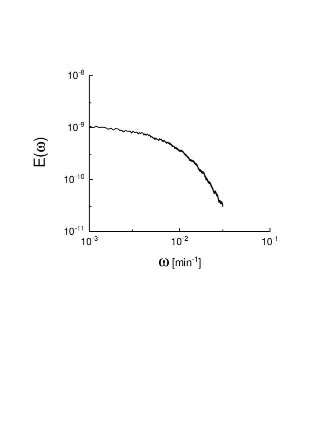
Figure 1: Spectrum of the X-ray flux raw data $I$ (in log-log scales).

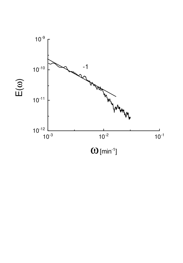
Figure 2: Spectrum of the X-ray flux data set, $I$, after exclusion of the points with the local dissipation rate $\epsilon>10^{-12}~{}W^{2}/cm^{4}s^{2}$. The straight line is drawn to indicate the ”-1” power law (2).

The straight line is drawn in figure 2 in order to indicate the power-law spectrum

$$E(\omega)\sim\omega^{-1}$$

in the log-log scales. For the discriminated data set (with the spectrum (2) at the low frequencies) we calculated moments of the local dissipation rate (1): $\langle\epsilon_{t}^{p}\rangle$. For the multiscale SOC (in particular for the 2D BTW model [11]) appearance of the multiscaling

$$\langle\epsilon_{t}^{p}\rangle\sim t^{-\mu_{p}}$$

is expected. Figure 3 shows the moments against $t$ (in log-log scales) and the straight lines are drawn in the figure in order to indicate the multiscaling (3). Slopes of these straight lines (best fit) provide us with multiscaling exponents $\mu_{p}$, which are shown in figure 4 as circles. The time interval where we observe the multiscaling of the dissipation field is: $10~{}min<Tt<1000~{}min$.

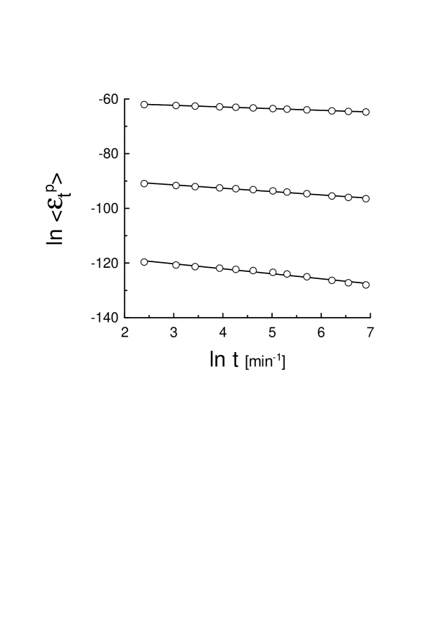
Figure 3: The local dissipation rate moments ($p=2,3,4$) against $t$ in log-log scales. The data set is the same that was used to obtain figure 2. The straight lines (the best fit) are drawn to indicate the multiscaling (3).

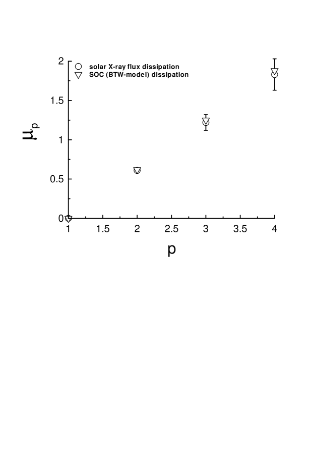
Figure 4: The multiscaling exponents $\mu_{p}$ (3) extracted as slopes of the straight lines in figure 3 (circles). Triangles correspond to the multiscaling exponents calculated in [11] for the 2D BTW model.

3 Discussion

The BTW prototype model of self-organized criticality is defined on a square lattice ($L\times L$) box [8]. On site $i$ $z_{i}=0,1,2,\ldots$ is the number of “grains”. If $z_{i}<4$, $\forall i$, the configuration is stable. Grain addition to a stable configuration is made by selecting at random a site $k$ where $z_{k}\to z_{k}+1$. If then $z_{k}\geq 4$, toppling occurs, i.e. $z_{k}\to z_{k}-4$, while each nearest neighbor, $l$, of site $k$ gets one grain ($z_{l}\to z_{l}+1$). If $k$ is at the border grains are dissipated. The toppling of site $k$ may cause instabilities in the neighbors, leading to further topplings at the next microscopic time step, and so on. Thus, an avalanche made by a total number $s\geq 0$ of topplings occurs before a new stable configuration is reached and a new grain is added. After many additions the system reaches a stationary critical state in which avalanche properties are sampled.

A key notion in the approach to the BTW is that of wave decomposition of avalanches [16]. The first wave is obtained as the set of all topplings which can take place as long as the site of addition is prevented from a possible second toppling. The second wave is constituted by the topplings occurring after the second toppling of the addition site takes place and before a third one is allowed, and so on. The total number of topplings in an avalanche is the sum of those of all its waves. The wave size has a pdf satisfying finite size scaling $P_{w}(s,L)\sim s^{-\tau_{w}}f_{w}(s/{L^{D_{w}}})$, where $\tau_{w}=1$, $D_{w}=2$, and $f_{w}$ is a suitable scaling function.

The multiscaling of the dissipation field

$$\epsilon_{t}=\sum_{k=1}^{t}(s_{k+1}-s_{k})^{2}/t$$

was observed in the Ref. [11] for the 2D BTW model and the multiscaling exponents for the BTW dissipation calculated in [11] are given in figure 4 as triangles. One can see good correspondence between the exponents calculated in [11] and the observed exponents.

The dissipation threshold $\epsilon\simeq 10^{-12}~{}W^{2}/cm^{4}s^{2}$, for which the solar X-ray data agree with the 2D BTW model both for the flux spectrum and for the dissipation multiscaling, corresponds to transition from the low intensity M-class flares to the high intensity M-class flares. At present time we do not know why just at this level of the dissipation rate the SOC (presumably BTW) mechanism overcomes all other mechanisms and appears so clear in the X-ray flux data. In any way, we can see that the multiscale SOC takes place there and even appears as a dominating mechanism at a certain stage.

The authors are grateful to the NOAA for providing the data.

References

- [1] E.N. Parker, Spontaneous Current Sheets in magnetic Fields, (Oxford Univ. Press, NY, 1994).
- [2] E. Liu and R.J. Hamilton, Astrophys. J., 380 L89 (1991).
- [3] P. Charbonneau, S.W. McIntosh, H-L. Liu, and T.J. Bogdan, Sol. Phys., 203, 321 (2001).
- [4] M.K. Georgoulis, N. Vilmer and N.B. Crosby, A&A, 367, 326 (2001).
- [5] D. Hughes, M. Paczuski, R.O. Dendy, P. Helander, and K.G. McClements, Phys. Rev. Lett., 90, 131101 (2003).
- [6] G. Boffeta, V. Carbone, P. Giuliani, P. Veltri and A. Vulpiani, Phys. Rev. Lett., 83, 4662 (1999).
- [7] P. Bak, C. Tang, and K. Wiesefeld, Phys. Rev. Lett., 59, 381 (1987).
- [8] D. Dhar, Physica A, 263, 4 (1999).
- [9] M. De Menech, and A.L. Stella, Phys. Rev. E, 58, R2677 (1998).
- [10] C. Tebaldi, M. De Menech, and A.L. Stella, Phys. Rev. Lett. 83, 3952 (1999).
- [11] M. De Menech and A.L. Stella, Physica A, 309, 289 (2002) (see also cond-mat/0103601).
- [12] J. Davidsen and M. Paczuski, Phys. Rev. E, 66, 050101(R) (2002).
- [13] R. Sánchez, D.E. Newman, and B.A. Carreras, Phys. Rev. Lett., 88, 068302 (2002).
- [14] A. Bershadskii, Phys. Rev. Lett., 90, 041101 (2003).
- [15] A.C Monin and A.M.Yaglom, Statistical fluid mechanics, Vol. 2 (MIT Press, Cambridge, 1975).
- [16] E.V. Ivashkevich, D.V. Ktitarev, and V.B. Priezzhev, Physica A, 209, 347 (1994).