Manuscript Title:
with Forced Linebreak

Non-Gaussian Signatures in the Lens Deformations of the CMB Sky. A New Ray-Tracing Procedure

Abstract

We work in the framework of an inflationary cold dark matter universe with cosmological constant, in which the cosmological inhomogeneities are considered as gravitational lenses for the CMB photons. This lensing deforms the angular distribution of the CMB maps in such a way that the induced deformations are not Gaussian. Our main goal is the estimation of the deviations with respect to Gaussianity appeared in the distribution of deformations. In the new approach used in this paper, matter is evolved with a particle-mesh N-body code and, then, an useful ray-tracing technique designed to calculate the correlations of the lens deformations induced by nonlinear structures is applied. Our approach is described in detail and tested. Various correlations are estimated at an appropriate angular scale. The resulting values point out both deviations with respect to Gaussian statistics and a low level of correlation in the lens deformations.

I Introduction

In the absence of a reionization, the photons of the Cosmic Microwave Background (CMB) are not scattered from decoupling to present time, except inside galaxy clusters (Sunyaev-Zel’dovich effect); nevertheless, the propagation direction of these photons changes due to the gravitational action of the cosmological inhomogeneities (lensing).

The so-called primary CMB anisotropies were produced by linear structures at high redshifts. The corresponding temperature contrast, $\Delta_{{}_{P}}\equiv(\Delta T/T)_{{}_{P}}$, is a statistical field which can be expanded in spherical harmonics as follows: $\Delta_{{}_{P}}=\sum_{m=-\ell}^{+\ell}a_{\ell m}Y_{\ell m}$, where the $a_{\ell m}$ quantities are statistically independent variables depending on the sky realization we are expanding. If many sky realizations are averaged, the resulting $a_{\ell m}$ coefficients have zero means and variances $\langle\mid a_{\ell m}\mid^{2}\rangle=C_{\ell}$. Since $\Delta_{{}_{P}}$ is a homogeneous and isotropic statistical field, quantities $\langle\mid a_{\ell m}\mid^{2}\rangle$ do not depend on $m$. In the model under consideration, scalar energy density fluctuations are initially Gaussian, and they remain Gaussian during linear evolution, by this reason, the primary CMB anisotropies –which were produced by linear inhomogeneities– also are Gaussian.

Gaussian primary anisotropy appears to be superimposed to secondary anisotropies generated well after decoupling, and also to the anisotropy of the microwave radiation emitted by both our galaxy and some extragalactic sources (contaminant foregrounds). These foregrounds are sub-dominant non Gaussian components contributing to the total observable signal at microwave wavelengths. In the model we are considering here, there are various secondary anisotropies. A few comments about them are worthwhile: the late integrated Sachs-Wolfe anisotropy was produced by quasi-linear inhomogeneities ful00 (1) and, consequently, deviations with respect to Gaussianity are not expected to be very important; another secondary gravitational anisotropy was produced by strongly nonlinear structures as galaxy clusters and substructures (Rees-Sciama effect), this component is sub-dominant and non Gaussian, and its deviations with respect to Gaussianity were studied by various authors mol95 (2, 3, 4); finally, the Sunyaev-Zeldovich anisotropy was produced by hot plasma in galaxy clusters, and it is also non Gaussian coo01 (5).

The main goal of this paper is the analysis of the non Gaussianity caused by lensing, and such an analysis can be performed using the operative ray-tracing procedure designed in next sections. In the absence of lensing, there are directional frequency shifts which cause an anisotropic temperature distribution in the CMB. The lens effect does no cause frequency shifts, but it produces angular deviations of the propagation directions. This means that the lens effect does not produce any alteration of the CMB temperature. It changes the propagation direction of the CMB photons and, then, the angular distribution of the CMB temperature changes accordingly. In other words, the lens effect deforms the maps of the CMB temperature which appear as a result of pure frequency shifts. Any numerical estimate of the alterations of the CMB maps produced by lensing (including non Gausianity generation) involves three steps: (i) maps of the CMB temperature distribution are built up for the model under consideration (without any lensing), (ii) these maps are deformed taking into account the deviations of the propagation directions produced by lensing, and (iii) the resulting deformations of unlensed maps (hereafter called either lens deformations or lens effect) are analyzed. Let us now consider each of these steps in more detail.

In order to built up unlensed maps of the CMB, we assume that, in the absence of lensing, the Gaussian primary anisotropy dominates and, consequently, the maps to be deformed can be built up using the angular power spectrum of this primary anisotropy, which has been calculated using CMBFAST seza96 (6) for the $\Lambda$CDM model under consideration. As it is discussed below, only small Gaussian maps having sizes of a few degrees and resolutions of the order of one arc-minute are necessary and they are built up using the Fourier Transform (FT) and the mentioned spectrum ($C_{\ell}$ quantities). See sae96 (7) and references cited therein for details. The resulting maps have spots with different sizes and amplitudes (angular structure). Spots with angular size $\pi/\ell$ have a mean amplitude proportional to $C_{\ell}^{1/2}$; hence, spots with angular size close to one degree ($\ell\sim 200$) have large amplitudes, whereas spots corresponding to one arcminute ($\ell\sim 10000$) have negligible amplitudes as a result of the smallness of $C_{10000}$. For the spectrum under consideration, significant spots have sizes of various arcminutes.

Cosmological inhomogeneities produce lensing and this effect is associated to the deviation field $\vec{\delta}$. The anisotropy observed in the $\vec{n}$ direction is the primary anisotropy corresponding to the direction $\vec{n}_{0}$ in the absence of lensing, where $\vec{n}=\vec{n}_{0}-\vec{\delta}$; hence,

$$\Delta(\vec{n})=\Delta_{{}_{P}}(\vec{n}_{0})=\Delta_{{}_{P}}(\vec{n}+\vec{\delta})\ .$$ (1)

The unit vectors $\vec{n}$ and $\vec{n}_{0}$ point towards two points of the last scattering surface, and the deviation field $\vec{\delta}$ gives the angular excursion on this surface due to lensing. We must estimate the deviation field $\vec{\delta}$ (see below) to get the deformed observable map $\Delta$. If the $\vec{\delta}$ deviations are smaller than the size of the smallest significant spots (various minutes), Eq. (1) can be expanded in $\vec{\delta}$ powers to get

$$\Delta(\vec{n})\simeq\Delta_{{}_{P}}(\vec{n})+\frac{\partial\Delta_{{}_{P}}}{\partial\vec{n}}\cdot\vec{\delta}$$ (2)

We see that map deformations, namely, the differences in the temperature contrasts corresponding to associate directions (second term of the r.h.s.) are the product of two statistical fields: $\Delta_{{}_{P}}$ and $\vec{\delta}$ and, even if these field are Gaussian and statistically independent, the resulting product would be non Gaussian.

Several authors have studied angular correlations in lensed CMB maps. In the most theoretical papers on this subject, some correlations have been estimated without using simulations; the approach used in these papers only applies for those correlations which can be written in terms of the time varying form of the matter power spectrum. In the most basic of these papers sel96 (8), the mentioned spectrum was modelled beyond the linear regime and the second order correlations of lensed CMB maps were estimated. A similar method was used by Bernardeau ber97 (9) to estimate fourth order correlations corresponding to various sets of four directions (with distinct configurations); furthermore, this last author pointed out that third order correlations vanish. Other methods are necessary to estimate correlations of order $n$ for $n>4$, and also to simulate CMB maps with the true statistics induced by lensing, namely, maps having the true correlations at any order (not only at second and fourth orders). The most powerful technique to study lens distortions in CMB maps is the use of ray-tracing through N-body simulations. Two methods to apply this tecnique are described in references jai00 (10) and whi01 (11) (other relevant papers in this field are cited in these two references). Another new method is proposed here. We agree with White & Hu whi01 (11), who stated that: ….. On subdegree scales, a full description of week lensing therefore requires numerical simulations, the most natural being N-body simulations ……; in fact, using ray-tracing through N-body simulations, CMB photons are deviated by fully nonlinear structures (as galaxy clusters) which move in the simulation box. Nowadays, only N-body simulations lead to a proper description of a distribution of strongly nonlinear structures. Unfortunately, these simulations constraint us to work in a periodic universe, and relevant problems associated to periodicity must be solved. Each method –designed to use ray-tracing through N-body simulations– corresponds to a different way for preventing periodicity effects. In this paper, one of these methods is described and tested.

Hereafter, quantity h is the reduced Hubble constant $h=10^{-2}H_{0}$, where $H_{0}$ is the Hubble constant in units of $Kms^{-1}Mpc^{-1}$, the density parameters corresponding to baryons, dark matter, and vacuum, are $\Omega_{b}$, $\Omega_{d}$ and $\Omega_{\Lambda}$, respectively, the total density parameter is $\Omega=\Omega_{b}+\Omega_{d}+\Omega_{\Lambda}$, and the matter density parameter is $\Omega_{m}=\Omega_{b}+\Omega_{d}$. In the flat inflationary universe under consideration, the above parameters take on the following values: $h=0.65$, $\Omega_{b}=0.05$, $\Omega_{d}=0.25$, and $\Omega_{\Lambda}=0.7$ and, then, according to Eke et al. eke96 (12), the power spectrum of scalar energy density perturbations must be normalized with $\sigma_{8}=0.93$ in order to have cluster abundances compatible with observations. Units are chosen in such a way that $c=8\pi G=1$, where $c$ is the speed of light and $G$ the gravitation constant. Whatever quantity ”$A$” may be, $A_{{}_{L}}$ and $A_{0}$ stand for the $A$ values on the last scattering surface and at present time, respectively. The scale factor is $a(t)$, where $t$ is the cosmological time, and its present value, $a_{0}$, is assumed to be unity, which is always possible in flat universes.

II Formalism

The CMB photons move on null geodesics and the line element is:

$$ds^{2}=-(1+2\phi)dt^{2}+(1-2\phi)a^{2}\delta_{ij}dx^{i}dx^{j}$$ (3)

where function $\phi$ satisfies the equation:

$$\Delta\phi=\frac{1}{2}a^{2}(\rho-\rho_{m0})\ ,$$ (4)

and $\rho_{m0}=\Omega_{m0}\rho_{crit}$ is the background energy density for matter. On account of this last equation, function $\phi$ can be interpreted as the peculiar gravitational potential created by the cosmological structures. Equations (3) and (4) are valid for linear inhomogeneities located well inside the horizon and also for nonlinear structures (potential approximation), see mar90 (13).

The deviation field $\vec{\delta}$ is given by the following integral sel96 (8):

$$\vec{\delta}=-2\int_{\lambda_{{}_{L}}}^{\lambda_{0}}W(\lambda)\vec{\nabla}_{\bot}\phi\ d\lambda\ ,$$ (5)

where $\vec{\nabla}_{\bot}\phi=-\vec{n}\wedge\vec{n}\wedge\vec{\nabla}\phi$ is the transverse gradient of the potential, and $W(\lambda)=(\lambda_{{}_{L}}-\lambda)/\lambda_{{}_{L}}$. The variable $\lambda$ is

$$\lambda(a)=H_{0}^{-1}\int_{a}^{1}\frac{db}{(\Omega_{m0}b+\Omega_{\Lambda}b^{4})^{1/2}}\ .$$ (6)

The integral in the r.h.s. of Eq. (5) is to be evaluated along the background null geodesics. In our flat background, the equations of the null geodesics passing by point $x^{i}_{{}_{P}}$ are:

$$x^{i}=x^{i}_{{}_{P}}+\lambda(a)n^{i}\ ,$$ (7)

In next section, spherical clusters with Navarro-Frenk-White (NFW) density profiles nav96 (14) are considered for qualitative analysis. These profiles appear in N-body simulations of dark matter halos and they have the form:

$$\rho(r)=\frac{\delta_{c}\ \rho_{m0}}{(r/r_{s})[1+(r/r_{s})]^{2}}\ ,$$ (8)

where $\rho_{m0}=\rho_{crit}\Omega_{m0}$, and $\rho_{crit}=3H^{2}$ is the critical density of the universe. The parameters $\delta_{c}$ and $r_{s}$ are related to both the concentration parameter $c_{{}_{NFW}}$ and the mass $M_{200}$. This mass is that contained inside a sphere whose mean density is $200$. The radius of this sphere is denoted $r_{200}$. The following relations hold:

$$r_{s}=(3M_{200}/800\pi\rho_{m0})^{1/3}/c_{{}_{NFW}}$$ (9)

$$\delta_{c}=\frac{200c_{{}_{NFW}}^{3}}{ln(1+c_{{}_{NFW}})-c_{{}_{NFW}}/(1+c_{{}_{NFW}})}\ .$$ (10)

The profile (8) remains almost unchanged from virialization ($z\sim 1$) to present time. Some authors have tried to assume the NFW profile with variable values of the involved parameters to go beyond virialization –until $z\sim 5$ in reference bul01 (15) –. Other authors use generalized profiles wyi01 (16). Fortunately, our qualitative analysis –presented in next section– does not require any detailed z-dependent profile.

In Sec. III, three clusters –which are hereafter called $C_{{}_{I}}$, $C_{{}_{II}}$, and $C_{{}_{III}}$– are considered. Cluster $C_{{}_{I}}$ is a rich one having $M_{200}=1000\ M_{g}$ (where $M_{g}=10^{12}\ M_{\odot}$) and $c_{{}_{NFW}}=6.8$, cluster $C_{{}_{II}}$ is a standard cluster having a few cents of galaxies with $M_{200}=250\ M_{g}$ and $c_{{}_{NFW}}=7.7$, and cluster $C_{{}_{III}}$ is a galaxy group having a few tens of galaxies with $M_{200}=25\ M_{g}$ and $c_{{}_{NFW}}=12.5$. Since the NFW profile diverges as physical radius $r$ tends to zero, an uniform core of radius $r_{c}$ has been assumed and, consequently, the density profile has the form (8) for $r\geq r_{c}$ and a constant value for $r\leq r_{c}$. Both profiles match continuously at $r=r_{c}$. For this mass distribution, function $d\phi/dr$ has the following form:

$$\frac{d\phi}{dr}=\frac{1}{6}\rho(r_{c})r$$ (11)

for $r\geq r_{c}$, where $\rho(r_{c})$ is given by Eq. (8), and

$$\frac{d\phi}{dr}=\frac{1}{r^{2}}[A+Dr_{s}^{3}\{E(r)-E(r_{c})\}]$$ (12)

for $r\leq r_{c}$, where $A=(1/6)r_{c}^{3}\rho(r_{c})$, $D=\delta_{c}\ \rho_{m0}/2$, and $E(r)=ln[1+(r/r_{s})]+[1+(r/r_{s})]^{-1}$. Core radius of $0.2\ Mpc$, $0.1\ Mpc$, and $0.05\ Mpc$ are assigned to clusters $C_{{}_{I}}$, $C_{{}_{II}}$, and $C_{{}_{III}}$, respectively. In next section, our conclusions are probed to be highly independent on this assignation.

Spherical linear inhomogeneities evolving inside the effective horizon are also considered in Sec. III for qualitative discussion. These spherical regions are assumed to be uniform and they are characterized by their comoving radius $R_{{}_{C}}$. This radius fixes the associated comoving scale $k_{{}_{C}}=\pi/2R_{{}_{C}}$ and, then, the present density contrast is fixed using the power spectrum of the energy density perturbations –in the model under consideration– which gives the average amplitude of the Fourier mode $k_{{}_{C}}$. The density contrast evolves proportional to the growing mode D(t), which is given in pee80 (17). Three of these linear inhomogeneities will be considered, they correspond to $R_{{}_{C}}=250\ Mpc$, $R_{{}_{C}}=50\ Mpc$, and $R_{{}_{C}}=12.5\ Mpc\sim 8h^{-1}\ Mpc$, and they are denoted $L_{{}_{I}}$, $L_{{}_{II}}$, and $L_{{}_{III}}$, respectively. The derivative of the gravitational potential with respect to the physical radius $r$ is

$$\frac{d\phi}{dr}=\frac{1}{6}(\rho-\rho_{m0})r$$ (13)

for $r\leq aR_{{}_{C}}$, and

$$\frac{d\phi}{dr}=\frac{a^{2}R_{{}_{C}}^{2}}{r^{2}}\frac{d\phi}{dr}(aR_{{}_{C}})$$ (14)

for $r>aR_{{}_{C}}$.

III Angular scales, boxes and resolution

Recently, various groups have used simulations of structure formation to estimate the effects of lensing on the CMB. An important problem is that there are many scales producing lensing and that, according to White & Hu whi01 (11), simulating the full range of scales implied is currently a practical impossibility. These authors proposed the tiling method to circumvent this problem and also the problems with periodicity (see Sec. I); this method employs many independent simulations with different boxes and resolutions to tile the photon trajectories. White & Hu whi01 (11) explained the advantages of their method with respect to the most traditional one based on plane projections, which has been extensively used in the literature (see jai00 (10) and references cited therein). The method proposed here does not require many independent simulations –but only one– and, consequently, it is simpler and numerically faster than the tiling one. Furthermore, it does not use plane projections whose potential problems were pointed out in whi01 (11). In this section, we are concerned with the scales relevant for CMB lensing, whereas periodicty is considered in next sections.

We are interested in the deviations with respect to Gaussianity produced by lensing jai00 (10). These deviations can be measured by angular correlations corresponding to three and more directions. Given an angular scale, the correlations are produced by a set of linear and nonlinear cosmological structures and, a detailed study of the type of structures contributing to these correlations is necessary in order to design our N-body simulations, which should include –in the same box– all the structures responsible for the effects we are looking for. In order to estimate scales, we can consider the evolving linear inhomogeneities $L_{{}_{I}}$, $L_{{}_{II}}$, and $L_{{}_{III}}$, and the nonevolving NFW density profiles $C_{{}_{I}}$, $C_{{}_{II}}$, and $C_{{}_{III}}$. Cluster evolution would not affect our qualitative estimates for small redshifts $z<5$, although it could be crucial in other contexts. In short, our study is based on six appropriate structures, three linear ones and three galaxy clusters.

Figure 1: Lens deviation $\delta$ as a function of the angle $\theta$ between the line of sight and the direction pointing towards the center of a spherical inhomogeneity. Top, middle, and bottom right (left) panels correspond to the linear structures $L_{{}_{I}}$, $L_{{}_{II}}$, and $L_{{}_{III}}$ (clusters $C_{{}_{I}}$, $C_{{}_{II}}$, and $C_{{}_{III}}$) defined in the text. In right (left) panel, solid, dotted, and dashed lines correspond to redshifts 2, 10, and 100 (0.5, 2, and 5), respectively. In the middle left panel, dotted-dashed (triple-dotted-dashed) line shows results for redshift 0.2 (0.1).

First of all, Eq. (5) and the potentials given in Sec. II have been used to calculate the lens deviations produced by the six selected structures. Each linear structure is placed at redshifts 2, 10 and 100, whereas each cluster is located at redshifts 0.5, 2 and 5 (cluster $C_{II}$ is also placed at $z=0.2$ and $z=0.1$). The deviation $\delta$ is calculated for each observation direction, which is characterized by the angle $\theta$ formed by the line of sight and the direction pointing towards the structure center. Results are presented in Fig. 1, where we see that: (i) the deviations grow as the redshift decreases, and the growing is small for $z\leqslant 0.5$ (compare the curves of the left middle panel of Fig. 1 corresponding to redshifts 0.5, 0.2 and 0.1), (ii) the deviations increase as the inhomogeneity size increases (this size is fixed by $M_{200}$ for clusters and by $R_{{}_{C}}$ for linear structures), (iii) small linear structures ($L_{{}_{III}}$) produces very small deviations whatever their location may be, (iv) small clusters (or groups, $C_{{}_{III}}$) produce a maximum deviation which is about $10$ % of the maximum deviation produced by cluster $C_{{}_{I}}$ (located at the same redshift), and (v) the most important deviations are produced by massive clusters and by very extended linear inhomogeneities.

Figure 2: Lens deformation, $d$, of the angle $\alpha$ formed by two directions pointing towards the same diameter of a spherical structure vs. the angle $\Theta$ defined in the text. This angle fixes the relative position of these directions with respect to the line of sight of the symmetry center. Solid lines of the top (bottom) panels correspond to cluster $C_{{}_{I}}$ at $z=0.5$ (the $L_{{}_{I}}$ inhomogeneity at $z=2$), whereas dotted lines correspond to the same redshifts but different structures $C_{{}_{II}}$ and $L_{{}_{II}}$ in all the panels. Dashed lines of the top panels are associated to cluster $C_{{}_{III}}$ at $z=0.5$. Left (right) panels give deviations for $\alpha=13.5^{\prime}$ ($\alpha=6.75^{\prime}$).

We are interested in the angular correlations of some CMB maps. Given a map of the variable $\zeta$ and $m$ directions, these correlations are defined as follows:

$$C_{m}=\langle\zeta(\vec{n}_{1})\zeta(\vec{n}_{2})\cdots\zeta(\vec{n}_{m})\rangle\ ,$$ (15)

where the average is over many realizations of the CMB sky. Some of these averages are estimated below for two, three and four directions in maps of both primary anisotropy and lens deformations. For $m=4$, the chosen directions draw the vertices of a square on the last scattering surface with $\vec{n}_{1}\cdot\vec{n}_{2}=\cos\alpha$, and for $m=3$, they point towards the vertices of an isosceles rectangle triangle with $\vec{n}_{1}\cdot\vec{n}_{2}=\cos\alpha$ and $\vec{n}_{1}\cdot\vec{n}_{3}=\cos\alpha$. The relevance of the deviations presented in the panels of Fig. 1 depends on the angular scale, $\alpha$, chosen for correlation computations. Suppose the scale $\alpha$ ($\ell=\pi/\alpha$) and $m=2$. From the primary temperatures corresponding to many pairs of directions ($\vec{n}_{1}$, $\vec{n}_{2}$) forming angle $\alpha$, the average $\langle\Delta_{{}_{P}}(\vec{n_{1}})\Delta_{{}_{P}}(\vec{n_{2}})\rangle$ can be calculated and the result measures correlations in the absence of lensing. According to Eq. (1), after lensing, the correlations are $\langle\Delta(\vec{n_{1}})\Delta(\vec{n_{2}})\rangle=\langle\Delta_{{}_{P}}(\vec{n_{01}})\Delta_{{}_{P}}(\vec{n_{02}})\rangle$ and, consequently, the correlations would change –due to lensing– if, as a result of deviations, the directions $\vec{n}_{01}$ and $\vec{n}_{02}$ form an angle $\alpha_{0}$ different enough from $\alpha$; therefore, in order to see if a certain spherical inhomogeneity located at redshift $z$ can contribute to the correlation at the angular scale $\alpha$, we may consider two directions pointing towards $R$ and $S$, two points of a certain diameter of the spherical structure; the first (second) of these directions forms angle $\theta$ ($\theta+\alpha$ ) with the direction of the symmetry center, and the angle $\Theta=\theta+\alpha/2$ corresponds to the middle point of the segment $RS$; then, the differences $d(\Theta)=\delta(\theta+\alpha)-\delta(\theta)$ measure the deformations of the angle formed by the two chosen directions. The top panels of Fig. 2 give these differences for the structures $C_{{}_{I}}$, $C_{{}_{II}}$, and $C_{{}_{III}}$ (at z=0.5), and the bottom panels for $L_{{}_{I}}$ and $L_{{}_{II}}$ (at z=2). The correlation scale is $\alpha=13.5^{\prime}$ ($\ell=800$) in the left panels and $\alpha=6.75^{\prime}$ ($\ell=1600$) in the right ones. From the analysis of this Figure it follows that: (a) big close clusters of type $C_{{}_{I}}$ produce the largest deformations reaching the maximum value $\sim 1.68^{\prime}$ ($\sim 1.98^{\prime}$) for $\alpha=13.5^{\prime}$ ($\alpha=6.75^{\prime}$), (b) for $\alpha=13.5^{\prime}$, inhomogeneities like $C_{{}_{II}}$, $C_{{}_{III}}$, $L_{{}_{I}}$, and $L_{{}_{II}}$ produce maximum deformations which are about $37.5\%$, $7.7\%$, $33\%$ and $6.8\%$ of the maximum ones corresponding to $C_{{}_{I}}$ clusters ($\sim 1.68^{\prime}$) and, (c) for $\alpha=6.75^{\prime}$, the maximum deformations produced by $C_{{}_{II}}$, $C_{{}_{III}}$, $L_{{}_{I}}$, and $L_{{}_{II}}$ structures are about $36.9\%$, $7.1\%$, $13.7\%$ and $2.9\%$ of the maximum deformation appearing in case $C_{{}_{I}}$ ($\sim 1.98^{\prime}$). Points (b) and (c) lead to the conclusion that the deformations produced by big linear structures are more important for $\alpha=13.5^{\prime}$, but they are not negligible in the case $\alpha=6.75^{\prime}$. The deformations corresponding to structures like $L_{{}_{III}}$ are too small and they have not been presented in Fig. 2.

From the above discussion, it follows that –for the scales under consideration– the most relevant structures are clusters of type $C_{{}_{I}}$ and $C_{{}_{II}}$ at low redshifts, and big linear inhomogeneities with $R_{{}_{C}}>50\ Mpc$ located at small redshifts. This conclusion is important. It tell us that simulations which do not resolve galaxy groups and small clusters can lead to good estimations, and also that the box size can be chosen to prevent the existence of extended linear inhomogeneities contributing to lensing. Boxes with sizes of $128\ Mpc$ should be appropriated, sizes of $256\ Mpc$ could be acceptable (although a part of the lensing could be due to linear structures with $R_{{}_{C}}>50\ Mpc$, see Sec. V) and, finally, boxes of $512\ Mpc$ and greater could contain an extended part of a $L_{{}_{I}}$ structure giving important contributions to lensing. The idea is that the lens effect produced by big linear inhomogeneities can be studied without simulations, see references in jai00 (10), whereas the effect of any other significant structure ($C_{{}_{I}}$ and $C_{{}_{II}}$ clusters) can be included in simulations for appropriate boxes (between $128\ Mpc$ and $256\ Mpc$ size). Let us now analyze if results from Figs. 1 and 2 are robust against variations of the core radius $r_{c}$.

Figure 3: Function $2W(\lambda)\vec{\nabla}_{\bot}\phi\times 10^{4}$ –involved in Eq. (5)– v.s. the comoving distance $\lambda-\lambda_{c}$ to the cluster center for the observation angle $\theta=2.5^{\prime}$. All clusters have been located at $z=0.5$. Each pair of associated solid and dotted lines corresponds to the cluster indicated inside the panel. Solid (dotted) line has been obtained from the greatest (smallest) values assigned to the core radius in the text.

Imagine one of the above three clusters located at redshift z. It produces a significant deviation of the CMB photons if and only if these photons cross the region where the function to be integrated in Eq. (5) (proportional to $\vec{\nabla}_{\bot}\phi$) is not negligible; hence, if the dependence of this function on the core radius is weak, lens deviations (integral in Eq. (5)) also depend weakly on $r_{c}$, and previous results based on Figs. 1 and 2 are robust. In order to study the mentioned function for clusters $C_{{}_{I}}$, $C_{{}_{II}}$, and $C_{{}_{III}}$, these structures are located at redshift 0.5 (where cluster evolution is not expected to be important) and, then, the function $d\delta(\theta)/d\lambda=2W(\lambda)\vec{\nabla}_{\bot}\phi$ involved in Eq. (5) is calculated at points of the null geodesic corresponding to the angle $\theta=2.5^{\prime}$. Results are presented in Fig. 3, where function $d\delta(2.5)/d\lambda$ is given (with arbitrary normalization) in terms of the comoving distance to the cluster center $\lambda-\lambda_{c}$, where $\lambda$ is the comoving distance from the observer to an arbitrary point of the null geodesic, and $\lambda_{c}$ is the $\lambda$ value corresponding to the cluster center. Continuous lines display the results obtained for clusters $C_{{}_{I}}$, $C_{{}_{II}}$, and $C_{{}_{III}}$ with the radius cores we have previously fixed, whereas the associated dotted lines correspond to the same clusters with smaller cores, the new core radius being $0.1\ Mpc$, $0.05\ Mpc$, and $0.025\ Mpc$ in cases $C_{{}_{I}}$, $C_{{}_{II}}$, and $C_{{}_{III}}$, respectively (the initially chosen radius have been reduced by a factor $1/2$).

The continuous and dotted associated lines of Fig. 3 are very similar for any cluster, which implies that, for $\theta=2.5^{\prime}$, the lens deviation $\delta$ has a very weak dependence on the core radius $r_{c}$. The direction $\theta=2.5^{\prime}$ has been arbitrarily chosen in the $\theta$ interval where the lens deformations are relevant (see Fig. 1); nevertheless, other angles covering this interval have been also studied. For example, we have investigated the directions corresponding to the maximum deviation in each of the cases reported in Fig. 1, and lens deviations also depends weakly on the core radius. The same occurs for any $\theta$ value, except for very small angles, which are not relevant for the angular scales under consideration (see below). In Fig. 3, we can also see that the region where $\vec{\nabla}_{\bot}\phi$ is significantly contributing to the integral of Eq. (5) has a comoving size of various Megaparsecs for any cluster of interest. It has been checked that the same conclusion is also valid for any relevant $\theta$ values.

A scale for the computation of angular correlations has been chosen. In order to do that, the CMB angular power spectrum ($C_{\ell}$ coefficients) due to lensing by nonlinear structures has been estimated using CMBFAST. Results lead to the conclusion that $C_{2}(\alpha)$ correlations from this lensing are important for $\alpha\leq 13.5^{\prime}$ ($\ell\geq 800$); hence we must work with some scale $\ell>800$. The scale $\ell=1600$ ($\alpha=6.75^{\prime}$) has been chosen to calculate correlations because this scale has the following properties: (a) for $\ell=1600$, the effect of linear inhomogeneities –which should be reduced as much as possible– is smaller than that of the case $\l=800$ (compare the bottom panels of Fig. 2), (b) according to CMBFAST estimations, lensing from nonlinear structures gives a $C_{1600}$ coefficient which is smaller than the maximum $C_{\ell}$ only by a factor $\sim 0.6$, and (c) the value $\ell=1600$ is in the range of the multipoles to be observed by PLANCK (the most sensitive projected experiment for CMB anisotropy measurements).

According to previous comments, a box of $128\ Mpc$ have been assumed as the basic one and, then N-body simulations have been performed inside this box with a standard PM code hoc88 (18), which was used, tested, and described in detail in qui98 (19). The resolution has been succesively increased starting from a very poor one of $2\ Mpc$. Of course, such a low resolution leads to non-linear structures whose amplitudes (sizes) are smaller (larger) than those of the true clusters. These simulations only traces a good spatial distribution of extended structures with total masses as those of the clusters (which would become clusters for appropriate resolutions). Resolutions of $1\ Mpc$ and $0.5\ Mpc$ have been also considered, but no higher resolutions have been used by the reasons given in Secs. V and VI.

IV Departures from Gaussianity

Suppose an observer which is located at a certain point with comoving spatial coordinates $x^{i}_{{}_{P}}$. The main question is: which is the deviation, $\vec{\delta}(\vec{x}_{{}_{P}},\vec{n})$, observed from point $\vec{x}_{{}_{P}}$ in the $\vec{n}$ direction?

If $\phi_{\vec{k}}(t)$ is the FT of the potential $\phi$, namely,

$$\phi(\vec{x},t)=\frac{1}{(2\pi)^{3/2}}\int d^{3}ke^{-i\vec{k}\cdot\vec{x}}\phi_{\vec{k}}(t)\ ,$$ (16)

and $\delta_{\vec{k}}$ is the FT of the density contrast $(\rho-\rho_{m0})/\rho_{m0}$, Equation (4) leads to the following relation in Fourier space: $\phi_{\vec{k}}=B\delta_{\vec{k}}/k^{2}$, where $B=-\rho_{m0}/a$.

Using elemental Fourier algebra and Eqs. (5), and (7), the following basic equations –giving the required deviation– are easily obtained:

$$\vec{\delta}(\vec{x}_{{}_{P}},\vec{n})=\frac{2i}{(2\pi)^{3/2}}\int\frac{\vec{k}_{\bot}}{k^{2}}F_{\vec{k}}(\vec{n})e^{-i\vec{k}\vec{x}_{{}_{P}}}d^{3}k\ ,$$ (17)

where

$$F_{\vec{k}}(\vec{n})=\int_{\lambda_{{}_{L}}}^{\lambda_{0}}W(\lambda)B(\lambda)e^{-i\lambda\vec{k}\vec{n}}\delta_{\vec{k}}(\lambda)d\lambda\ ,$$ (18)

and $\vec{k}_{\bot}=\vec{k}-(\vec{n}\cdot\vec{k})\vec{n}$.

According to Eq. (17), each component of $\vec{\delta}(\vec{x}_{{}_{P}},\vec{n})$ is the FT –extended to all the space– of a component of vector $\vec{k}_{\bot}F_{\vec{k}}(\vec{n})/k^{2}$. The integral of the r.h.s. of Eq. (18) must be estimated to get the function $F_{\vec{k}}(\vec{n})$ involved in the FT. The integration variable $\lambda$ can be seen as a generalized time coordinate. Equations (17) and (18) are general and they describe how the photons deviate –following null geodesics– in a realization of the full universe; nevertheless, such a realization is not available in practice, and we are constrained to use these equations in a fictitious periodic universe, let us now discuss this fact and its consequences in detail.

Structure evolution is simulated with a certain N-body code (see Sec. III), which involves a box and a certain resolution (a network in position space). This code has a certain time step (or $\lambda$ step) and, consequently, it gives data at a set of time values; among these data, we are particularly interested in the function $\delta_{\vec{k}}(\lambda)$ which appears in Eq. (18). This function is easily evaluated at each node, $\vec{k}$, in Fourier space, and at each time step $t_{i}$, but not at arbitrary times. The question is: Can we calculate the integral (18) using only the data corresponding to the time discretisation of the N-body code? Fortunately, the answer is positive. We have studied the function $\delta_{\vec{k}}(\lambda)$ for many $\vec{k}$ values and, thus, we have verified that the term $I(\vec{k},\lambda)=W(\lambda)B(\lambda)\delta_{\vec{k}}(\lambda)$ –which appears in Eq. (18)– can be very well approximated by a straight line between $\lambda_{i}$ and $\lambda_{i+1}$, namely, between two successive time steps of the N-body simulation. The equation of this line is of the form:

$$I_{i}(\vec{k},\lambda)=A_{i}(\vec{k})\lambda+B_{i}(\vec{k})$$ (19)

where quantities $A_{i}$ and $B_{i}$ are obtained from $\delta_{\vec{k}}(\lambda_{i})$ and $\delta_{\vec{k}}(\lambda_{i+1})$; namely, from quantities given by the N-body in two successive steps. If Eq. (19) is substituted into Eq. (18), the integral of the r.h.s. can be analytically calculated in the interval ($t_{i},t_{i+1}$). The addition of these integrals for all the N-body intervals gives function $F_{\vec{k}}(\vec{n})$. After this integration, the FT (17) can be performed and, thus, the deviation field in the $\vec{n}$ direction is simultaneously calculated for many observers located at the nodes $\vec{x}_{{}_{P}}$ of the spatial Fourier box. The importance of this fact is discussed below.

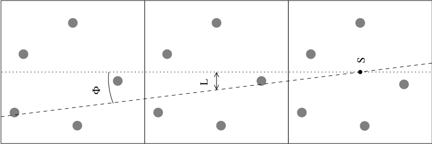
Figure 4: Sketch of a 2D universe filled by squares which contains clusters (circles) and photon patches (lines). Dotted (dashed) line corresponds to a direction parallel (non parallel) to the square edges.

Discretisation implies that the CMB photons do not move in a true realization of the universe, but in a periodic universe, which is, at each time, an ensemble of boxes identical to that of the N-body simulation. This periodicity should lead to errors in our estimations. In order to understand the problem and its solution, let us establish a two-dimensional (2D) analogy. The squares of Fig. 4 (boxes in the 3D case) have a size of $128\ Mpc$. These squares contain small circles (clusters), and let us imagine an observer, S, at the center of the right square. If a photon propagates along the pointed line of Fig. 4, it crosses all the squares in the same way, namely, it passes at the same distances from the same clusters and undergoes the same systematic repeated deviations. Only evolution induces small deformations from square to square, but these deformations would be only relevant after a large enough number of squares have been crossed; hence, a certain wrong accumulative effect should appear. However, if the photon moves following the dashed line of Fig. 4, the situation is very different because the photon enters each square around a very different place and, then, it can be affected by distinct independent clusters. The key point is the selection of the angle $\Phi$ and its associate distance $L$. Two facts are relevant to make this choice: (i) clusters significantly deviate the CMB photons when their impact parameter is smaller than a few Megaparsecs (see Fig. 3), and (ii) correlations in the cluster distribution (superclusters) extend near $10\ Mpc$; hence, if we choose $L$ between $15\ Mpc$ and $20\ Mpc$, photons move from square to square, but they are always influenced by different almost uncorrelated clusters and, consequently, the effect of periodicity must be minimum. All these considerations are easily generalized to the 3D case, in which there are two angles defining the line of sight. Hereafter, these angles are identified with the spherical coordinates $\theta$ and $\phi$ (with respect to the Cartesian axis defined by the edges of the box). These angles can be easily chosen to maximize the length of the path where the photons undergo the action of distinct uncorrelated clusters; namely, to minimize the effects of periodicity. In the 3D case, with boxes of $128\ Mpc$, it has been found that for $\theta=10.75^{\circ}$ and $\phi=41.19^{\circ}$, the photons would cross 56 boxes before arriving to the initial region of the box. The CMB photons moving along this direction (hereafter denoted $\vec{N}_{0}$ and called the preferred direction) do not feel periodicity during their travel from $r\simeq 7400\ Mpc$ to $r=0$, namely, from $z=3.62$ to $z=0$ and, taking into account that the lens effect we are evaluating is produced at these low redshifts by galaxy clusters, it follows that, for direction $\vec{N}_{0}$ and close ones, periodicity must be rather irrelevant (see Sec. V for more discussion). Furthermore, the photon enters in two successive boxes through points that –when placed in a unique box– are located at a distance $L=15.9\ Mpc$. For the chosen values of $\theta$ and $\phi$ and a box of $256\ Mpc$, we have $L=31.8\ Mpc$, and photons does not feel periodicity at all from decoupling to present time.

On the angular scales under consideration, the cluster distribution producing lensing is statistically independent on the structure distribution causing the primary anisotropy; in fact, for $\alpha$ values between $6.75^{\prime}$ and $13.5^{\prime}$ ($1600\geq\ell\geq 800$), primary anisotropy is due to temperature fluctuations previous to decoupling, which appeared as a result of the coupling between matter an radiation in the presence of energy density fluctuations; hence, the scales of temperature fluctuations and those of energy perturbations coincide. Inhomogeneities with a comoving size of $41\ Mpc$ ($20.5\ Mpc$) located at $z=1100$ subtend an angle of $13.5^{\prime}$ ($6.75^{\prime}$); hence, taking into account that –in our $\Lambda$CDM model– the comoving scale of an Abell cluster with $10^{15}M_{\odot}$ is $25.6\ Mpc$, we can conclude that, for $800\leq\ell\leq 1600$, the primary anisotropy is produced by comoving scales similar to those of clusters. These small structures located close to our last scattering surface ($z\sim 1100$) and the clusters producing lensing (small $z$ values) are very far, different, and independent structure distributions; therefore, we can consider that the distribution of clusters is producing deformations on independent primary CMB maps. In order to calculate the averages of Eq. (15) (correlations), various full realizations of the cluster distribution should be considered to produce deviation fields and, then, each of these fields should be used to deform a large enough number of independent primary maps. In practice (computational limitations), only a few pairs of directions (close to $\vec{N}_{0}$ to minimize periodicity effects) are studied for each cluster distribution (N-body simulation), and these directions should be used to deform different primary maps. Let us now describe in detail the method implemented in this paper to calculate correlations.

For each N-body simulation, nine directions $\vec{n}_{i}$ are considered. These directions are chosen in such a way that they depict the vertices of four neighboring squares with size $\alpha$ on the last scattering surface. These squares form another bigger one with size $2\alpha$ with vector $\vec{N}_{0}$ pointing towards its center. It is important that, for each of the chosen directions, the deviations $\vec{\delta}(\vec{x}_{{}_{P}},\vec{n}_{i})$ are calculated for the $N^{3}$ observers, $\vec{x}_{{}_{P}}$, at the same time (see above). Let us discuss the importance of this fact from the statistical point of view. Put a $4.25^{\circ}\times 4.25^{\circ}$ map, $M_{{}_{P}}$, of primary anisotropy in such a way that, from the box center (point $\vec{x}_{{}_{C}}$), the direction $\vec{N}_{0}$ points towards the map center $C$. Consider now one of the observation direction $\vec{n}_{i}$. From the box center, the chosen direction points towards a certain point $C_{i}$; nevertheless, from another point of the box $\vec{x}_{{}_{Q}}$, direction $\vec{n}_{i}$ does not point towards point $C_{i}$ but towards another point $Q_{i}$ of the map $M_{{}_{P}}$. Two parallel lines –with direction $\vec{n}_{i}$– starting from points $\vec{x}_{{}_{C}}$ and $\vec{x}_{{}_{Q}}$ of the box would intersect the map $M_{{}_{P}}$ in points $C_{i}$ and $Q_{i}$, respectively; hence, the $Q_{i}$ coordinates in the map $M_{{}_{P}}$ can be calculated as follows: project the vector $\vec{x}_{{}_{Q}}-\vec{x}_{{}_{C}}$ on the plane normal to $\vec{n}_{i}$, translate this projection parallely from the hypersurface $t=0$ to the last scattering surface at $z=1100$, calculate the angle subtended by the final vector (as it is seen by the observers) and, then, the angular coordinates of point $Q_{i}$ in the map $M_{{}_{P}}$ can be trivially obtained. Of course, the deviation, $\vec{\delta}(\vec{x}_{{}_{Q}},\vec{n}_{i})$, corresponding to the observer $\vec{x}_{{}_{Q}}$ in the direction $\vec{n}_{i}$, must be applied to point $Q_{i}$ in the map $M_{{}_{P}}$. Hence, for each direction $\vec{n}_{i}$, we have not a unique point in $M_{{}_{P}}$, but many points, one for each $\vec{x}_{{}_{Q}}$ observer, and these points cover a certain region on map $M_{{}_{P}}$. In order to estimate the size of the covered region, we can consider a fixed direction, for example $\vec{n}=(0,0,1)$, and a box of $128\ Mpc$ ($256\ Mpc$) per edge; thus, given two observers $\vec{x}_{{}_{Q1}}$ and $\vec{x}_{{}_{Q2}}$ separated by a distance of $128\ Mpc$ ($256\ Mpc$), the angular distance between points $Q_{1}$ and $Q_{2}$ in the map $M_{{}_{P}}$ appears to be $\Xi=0.5^{\circ}$ ($\Xi=1^{\circ}$), which means that, for $\alpha=13.5^{\prime}$, a squared region with a size of $43.5^{\prime}$ ($73.5^{\prime}$) is covered, and for $\alpha=6.75^{\prime}$, the size of the corresponding region is $36.75^{\prime}$ ($66.75^{\prime}$); hence, we see that, for boxes of $128\ Mpc$ ($256\ Mpc$) and $\alpha=6.75^{\prime}$, the size of this region is larger than $\alpha$ by a factor close to five (ten) and, consequently, the averages in the $\vec{x}_{{}_{Q}}$ observers –a novel aspect of our ray-tracing procedure– play a crucial statistical role. The greater the boxes and the smaller the angular scales $\alpha$, the larger the above factor and the greater the statistical significance of the $\vec{x}_{{}_{Q}}$ averages.

On account of the above considerations, correlations are calculated as follows: (i) twelve different pairs of directions, sixteen triads, and four tetrads are defined using the above nine directions, (ii) given an observer $\vec{x}_{{}_{Q}}$, a map $M_{{}_{P}}$ (primary anisotropy), and a N-body simulation (for $\vec{\delta}$ computation), the deviations $\vec{\delta}(\vec{x}_{{}_{Q}},\vec{n}_{i})$ and Eq. (1) (or Eq. (2)) are used to calculate the lens effect $\Delta[\vec{n}_{i}+\vec{\delta}(\vec{x}_{{}_{Q}},\vec{n}_{i})]-\Delta[\vec{n}_{i}]$ (or $\vec{\delta}(\vec{x}_{{}_{Q}},\vec{n}_{i})\cdot[\partial\Delta_{{}_{P}}/\partial\vec{n}]_{\vec{n}_{i}}$) for each of the $\vec{n}_{i}$ directions and, then, the resulting data are used to compute the averages (15) for the above pairs ($m=2$), triads ($m=3$), and tetrads ($m=4$), (iii) calculations in (ii) are repeated for each observer $\vec{x}_{{}_{Q}}$, and results are averaged again, (iv) all the process is repeated for a certain number of $M_{{}_{P}}$ maps and a new average is performed and, (v) finally, the above calculations are repeated for a certain number of N-body simulations, and the final averages are taken as our estimations of the correlations (15). The question is: How many primary maps and how many cluster realizations would be necessary to calculate the required correlations?

In order to answer this question, the following method has been implemented: In a first step, the process (i)-(iv) has been used to analyze pure primary maps in the absence of lens deviations. The primary maps are not deformed and, consequently, the resulting averages should approach the true two, three, and four direction correlations of these maps, which are hereafter called primary correlations. These correlations can be estimated by a direct analysis of the simulated primary maps (see next section) and the results of such an analysis can be compared with the correlations estimated by the process (i)-(iv) in the absence of deviations. Since no deviations have been considered, this study measures the capability of our method (based on nine direction, $N^{3}$ observers, and various primary maps) to create pairs, triads and tetrads covering a significant part of the primary maps; namely, allowing a good statistical analysis of maps. In the second and final step, the number of primary maps suggested by our previous study (in the absence of deviations) is taken and, then, deviations from more and more N-body simulations are considered in order to compute the required correlations as it has been described above. When the averages reach almost stable values, the process is stopped and no more N-body realizations are performed. Results are presented in next section.

Figure 5: Correlations $C_{2}$, $C_{3}$, and $C_{4}$ extracted from simulated maps of the primary CMB anisotropy (for $\alpha=6.75^{\prime}$), versus the number $N_{p}$ of simulated maps used in the computations. Left, central, and right panels show the correlations $C_{2}$, $C_{3}$, and $C_{4}$, respectively. Different curves correspond to distinct methods for correlation estimates which are described in the text.

V Results

First of all, the methods applied –in this paper– to calculate correlations of the lens effect are tested. In order to do that, these methods are used to analyze well known maps of primary anisotropy. The angular scale for correlation estimates is $\alpha=6.75^{\prime}$. A set of two hundred maps of primary anisotropy has been used. Results are presented in Fig. 5, where variable $N_{p}$ (horizontal axis) is the number of primary maps used to get the correlation value appearing in the vertical axis. Left, central, and right panels correspond to the two ($m=2$), three ($m=3$) and four ($m=4$) direction correlations (15), respectively. In all the panels, the solid line shows the correlations obtained by means of an exhaustive coverage of the $M_{{}_{P}}$ maps using many pairs, triads and tetrads of directions. This is our best estimate of the required correlations; results from this method –which cannot be applied to analyze the lens component– approach the theoretical values of the correlations we have used to simulate the $M_{{}_{P}}$ maps. Other methods must give similar correlations to be acceptable. As $N_{p}$ increases, the solid lines of the top and bottom panels seem to tend to a certain value, whereas the continuous line of the middle panel seems to be compatible with a vanishing $C_{3}$ correlation. The long dashed lines display the correlations obtained using nine directions and only one observer (only nine directions in each map). These lines slowly approaches the solid one as $N_{p}$ increases and the level of approximation seems to be good for $N_{p}=200$. The dotted (dashed) lines give the correlations obtained with nine directions and $128^{3}$ ($256^{3}$) observers. As it follows from Fig. 5, dashed and dotted curves approach the solid ones faster than the long dashed lines and, consequently, the use of many observers located in the nodes of a network (see Sec. IV) is statistically significant; the greater the box size, the faster the statistical approximation to the solid lines. The best situation corresponds to $256^{3}$ observers in a $256\ Mpc$ box. Two hundred primary maps suffice for a good enough estimate of $C_{2}(6.75)$ and $C_{4}(6.75)$; particularly, when $N^{3}$ observers are considered.

After computing the correlations $C_{2}(6.75)$, $C_{3}(6.75)$, and $C_{4}(6.75)$ for lens deformations, it would be worthwhile a comparison between the correlation level of these deformations and that of primary maps. The ratios $r_{2}=C_{2}(6.75)/C_{2}(0)$, $r_{3}=C_{3}(6.75)/C_{2}^{3/2}(0)$, and $r_{4}=C_{4}(6.75)/C_{2}^{2}(0)$ are apropriate to do this comparison; these quantities will be calculated for lens deformations and primary maps and, then, results will be compared. We begin with the case of primary maps. Using two hundred of these maps and exhaustive coverage, we have found: $C_{1}=\langle\Delta_{{}_{P}}(\vec{n})\rangle=-2.12\times 10^{-6}$, $C_{2}(0)=\langle\Delta_{{}_{P}}(\vec{n})\Delta_{{}_{P}}(\vec{n})\rangle=7.29\times 10^{-8}$, and $r_{1}=C_{1}/C_{2}^{1/2}(0)=7.85\times 10^{-3}$. We know that there are many positive and negative temperature contrasts –in the maps– with absolute values close to $C_{2}^{1/2}(0)$ and, consequently, only an strong cancellation of these contrasts can explain the resulting value of the mean contrast $C_{1}(0)$, which is much smaller than $C_{2}^{1/2}(0)$ (small ratio $r_{1}\sim 7.9\times 10^{-3}$). Strong cancellation leading to a small $r_{1}$ value indicates that, as the number of maps increases, quantity $\langle\Delta_{{}_{P}}(\vec{n})\rangle$ approaches either a small value or zero. Similarly, in order to calculate the correlation $C_{2}(6.75)=\langle\Delta_{{}_{P}}(\vec{n_{1}})\Delta_{{}_{P}}(\vec{n_{2}})\rangle$, positive and negative numbers with absolute values close to $C_{2}(0)$ are averaged. The resulting ratio $r_{2}\sim 0.85$ indicates that these numbers have not cancelled among them and a nonvanishing $C_{2}(6.75)$ correlation exists. For $m=3$ (m=4), the relevant ratio is $r_{3}\sim 8.8\times 10^{-3}$ ($r_{4}\sim 2$) and, this small (large) ratio $r_{3}$ ($r_{4}$) strongly suggests a vanishing $C_{3}$ (significant $C_{4}$) correlation.

Since the simulated primary maps are Gaussian, the relations $C_{3}(6.75)=0$ and $C_{4}(6.75)=3C_{2}^{2}(6.75)$ must be satisfied. The correlation $C_{3}$ obtained by exhaustive coverage (solid lines of Fig. 5) is $C_{3}\simeq-1.76\times 10^{-13}$, and it has been proved to be small by computing $r_{3}$; furthermore, we have used the same method to get the correlations $C_{2}\simeq 6.24\times 10^{-8}$ and $C_{4}\simeq 1.09\times 10^{-14}$, which lead to the ratio $3C_{2}^{2}/C_{4}\simeq 1.07$; hence, we can say that the correlations extracted from the maps are compatible with Gaussianity, as it should be for the primary maps we are analyzing. If we use other methods to analyze the $M_{p}$ maps; for example, the methods used to built up the dotted, dashed, and long dashed curves of Fig. 5 (see above), the extracted correlations appear to be similar to those reported above and so they are compatible with Gaussianity; this means that all the methods used to analyze maps work very well for primary maps, and the same should occur in our applications to the analysis of lens deformations.

Figure 6: Correlations $C_{2}$, $C_{3}$, and $C_{4}$ extracted from simulated maps of the lens effect (for $\alpha=6.75^{\prime}$), versus the number $N$ of simulated maps used in the calculations. Top, middle, and bottom panels show the correlations $C_{2}$, $C_{3}$, and $C_{4}$, respectively. solid, dashed, and dotted lines of the left panels corresponds to resolutions of $0.5\ Mpc$, $1\ Mpc$, and $2\ Mpc$, respectively. Dashed (solid) lines of the right panels show correlations for direction close to the preferred one (a direction parallel to an edge of the simulation box).

Table 1: Correlations in simulated lens deformations of the CMB sky.

Case	Box Size	Resolution	Direction	$C_{2}\times 10^{11}$	$C_{3}\times 10^{18}$	$C_{4}\times 10^{21}$
	in Mpc	in Mpc
1	128	0.5	optimal	3.59 $\pm$ 0.12	$-$1.10 $\pm$ 0.14	2.71 $\pm$ 0.18
2	128	1.0	optimal	3.57 $\pm$ 0.06	$-$1.40 $\pm$ 0.18	2.70 $\pm$ 0.10
3	128	2.0	optimal	3.27 $\pm$ 0.06	$-$2.63 $\pm$ 0.24	2.28 $\pm$ 0.08
4	128	1.0	parallel to an edge	2.50 $\pm$ 0.02	$-$1.43 $\pm$ 0.16	1.05 $\pm$ 0.03
5	256	1.0	optimal	3.08 $\pm$ 0.06	$-$0.76 $\pm$ 0.06	2.07 $\pm$ 0.08

Correlations of lens deformations have been calculated in various cases using distinct PM simulations; in case 1, the resolution is $0.5\ Mpc$ (the best one), the box size is $128\ Mpc$, directions are close to the preferred one, and the angular scale is $\alpha=6.75^{\prime}$. Correlations obtained in this case are presented in the first row of table 1, and also in the continuous lines of the left panels of Fig. 6. All the data of table 1 are mean correlations with $2\sigma$ errors calculated from the correlations of forty simulations. These errors are statistical ones assigned in case 1, but there are other sources of uncertainty as periodicity and simulation features, which are not included in the errors reported in table 1. The lines mentioned above display the variation of the estimated correlations as the number N of simulations (used to perform averages) increases; for $N>20$, correlations $C_{2}$ and $C_{4}$ seem to coverge towards a certain value, whereas the correlation $C_{3}$ slowly decreases in the $N$-interval (20,40) (see continuous lines in the middle panels of Fig. 6, which are two different representations of the same function). We assign to $C_{2}$, $C_{3}$, and $C_{4}$ the values and errors given in the first row of table 1; the tabulated values of $C_{2}$ and $C_{4}$ are estimations of these correlations, whereas that of $C_{3}$ can be better considered as an upper limit due to the slow decreasing we have mentioned above. The values assigned to $C_{2}$, $C_{3}$, and $C_{4}$ have been used to calculate the ratios $r_{2}\simeq 0.081$, $r_{3}\simeq 1.17\times 10^{-4}$, and $r_{4}\simeq 0.014$, which are smaller than the corresponding ratios of the primary maps (see above). The small $r_{3}$ value indicates that lensing (by nonlinear structures) does not introduce any appreciable $C_{3}$ correlation, whereas the small values of $C_{2}$ and $C_{4}$ suggest small levels of these correlations. Finally, the ratio $3C_{2}^{2}/C_{4}\simeq 1.43$ confirms a deviation with respect to Gaussianity.

Table 2: Comparing lens correlations for various pairs of estimations.

Compared Cases	$100\Delta C_{2}/C_{2}$	$100\Delta C_{3}/C_{3}$	$100\Delta C_{4}/C_{4}$
1-2	0.56	21.	0.37
2-3	8.91	58.	16.
2-4	30	2.09	61
2-5	13.73	46	23

Since the method proposed in previous sections is based on N-body simulations, results could depend on both resolution and box size. These dependences are now studied. In order to analyze the importance of resolution, cases 2 and 3 have been considered, they are identical to the case 1 described above except for resolution, which is $0.5\ Mpc$ in case 1, $1.\ Mpc$ in case 2, and $2.\ Mpc$ in case 3. Results of case 2 (3) are displayed in the second (third) row of table 1, and also in the dashed (dotted) lines of the left panels of Fig. 6, where we see that the correlations $C_{2}$, $C_{3}$, and $C_{4}$ of case 3 ($2.\ Mpc$ resolution) are smaller than those of case 2 ($1.\ Mpc$) and case 1 ($0.5\ Mpc$), which are very similar between them. In order to quantify these comparisons between results corresponding to pairs of cases, the relative variations $\Delta C_{m}/C_{m}$ for $m=2,3,4$ are obtained for the pairs 1-2 and 2-3, and the comparation percentages $100\Delta C_{m}/C_{m}$ for these pairs are given in the first and second rows of table 2, where we see that the comparation percentages of the pair 1-2 are much smaller than those of 2-3. These considerations strongly suggests that a $2.\ Mpc$ resolution is poor, whereas a $1.\ Mpc$ resolution is good because a better one ($0.5\ Mpc$) does not lead to significantly better results; particularly, for the correlations $C_{2}$ ($100\Delta C_{2}/C_{2}=0.56$ for cases 1-2) and $C_{4}$ ($100\Delta C_{4}/C_{4}=0.37$ for cases 1-2). Taking into account that cluster description can be improved using higher resolutions, these results have two possible interpretations: (1) the calculation of the lens correlations does not require a more detailed description of the clusters (for the chosen angular scale $\alpha=6.75^{\prime}$) and, (2) results from resolutions of $1\ Mpc$ and $0.5\ Mpc$ are similar because of a lack of resolution in both cases, but higher resolutions would lead to –different– better results. We have not found any theoretical reason supporting one of these alternatives. In this situation, the most effective procedure is the use of new simulations with higher resolutions, which should support one of the above possibilities (see Sec. VI for more discussion).

After concluding that a resolution of $1.\ Mpc$ seems to be good (at least it is equivalent to a better resolution of $0.5\ Mpc$), and before analyzing the importance of the box size, a study of the relevance of periodicity is worthwhile. In order to perform such a study, results of case 2 are compared with those of case 4. In both cases, the same forty simulations are used, but the propagation directions of the CMB photons are different. In cases 2 and 4, directions form small angles with the preferred direction and with an edge of the simulation box, respectively. Results of case 4 are displayed in the forth row of table 1, and also in the solid line of the right panels of Fig. 6 (where dashed lines correspond to case 2). Comparing the solid and dashed lines of these panels, one easily concludes that periodicity strongly (weakly) affects the correlations $C_{2}$ and $C_{4}$ ($C_{3}$). Accordingly, the comparation percentages of the correlations $C_{2}$ and $C_{4}$ for the pair of cases 2-4 (third row of table 2) are much greater than that of the $C_{3}$ correlation, which appears to be as small as $2.09\%$. This dependence of $C_{2}$ and $C_{4}$ on the direction constraints us to work with directions close to the preferred one, which strongly minimizes periodicity effects (see Sec. IV).

Figure 7: Same as Fig. 6 for box sizes of $128\ Mpc$ (dashed lines) and $256\ Mpc$ (solid lines).

Finally, results of case 2 are compared with those of case 5 to analyze the importance of the box size. Case 5 is identical to case 2 except for this size, which takes on the values $256\ Mpc$ and $128\ Mpc$ in cases 5 and 2, respectively. Possible differences between cases 2 and 5 can be explained in two different ways: (i) boxes of $256\ Mpc$ contain linear inhomogeneities more extended than those involved in boxes of $128\ Mpc$ and, according to our discussion of Sec. III, linear inhomogeneities with different sizes produce distinct lensing and, (ii) there is a residual effect of periodicity, which would depend on box size for the fixed preferred direction used in our calculations (initially associated to $128\ Mpc$ boxes, see Sec. IV). Results of case 5 are shown in the fifth row of table 1, and also in the solid lines of Fig. 7 (where dashed lines correspond to case 2). Comparing the solid and dashed lines of Fig. 7, and taking into account that the comparation percentages of the pair 2-5 (forth row of table 2) are $13.73\%$ for $C_{2}$, $46\%$ for $C_{3}$, and $23\%$ for $C_{4}$, we conclude that box size is important. Is that due to residual periodicity? The answer to this question is negative because the comparation percentage in $C_{3}$ due to periodicity has been proved to be very small ($2.09\%$), whereas the corresponding percentage has appeared to be $46\%$ when the box size has been varied. Hence, the box size is important as a result of the presence of large scale inhomogeneities and, consequently, our best estimate of the correlations induced by nonlinear lensing corresponds to the smallest box size ($128\ Mpc$) and the best resolution ($0.5\ Mpc$) we have used (case 1). The comparation percentages of the pair 2-5 are not to be confused with the error percentages in the correlations of case 2, which would be expected to be smaller, perhaps about a few per cent. The same has occurred for resolution, where the comparation percentages of the pair 2-3 (second row of table 2) are much larger than the error percentages of case 2 (comparable to the quantities in the first row of table 2).

VI Discussion

A ray-tracing method to calculate correlations in lens deformations of CMB maps has been designed, tested, and applied. It is based on the use of PM N-body simulations to evolve nonlinear cosmological structures. Although correlations are calculated from the deformations associated to a reduced number of directions (no complete maps of deformations are created), numerical calculations are time consuming because a large enough number of N-body simulations must be performed to calculate good statistical averages (correlations). The method is similar to that proposed by Aliaga et al. ali02 (4) to study the Rees-Sciama effect, and it can be easily implemented starting from an N-body code.

Firts of all, the main structures producing lens deformations in the CMB sky have been identified. A qualitative estimation of the lens deformations produced by a representative set of linear and nonlinear cosmological structures has been used to achieve this identification. Various reasons have motivated the choice of the angular scale $\alpha=6.75^{\prime}$ to compute correlations (see Sec. III). For this scale, it has been proved that lens deformations are mainly produced by big and standard clusters, although there is a moderate contribution from linear inhomogeneities with diameters greater than $100\ Mpc$. This information has been crucial to choose the N-body simulations in such a way that the effect of the linear inhomogeneities contained in the simulation box is much smaller than that of the nonlinear structures. Using these simulations, the deviation field $\vec{\delta}$ produced by nonlinear structures can be numerically estimated and, independently, the field $\vec{\delta}$ due to large scale linear inhomogeneities can be analytically calculated. Qualitative arguments suggest that box sizes between $128\ Mpc$ and $256\ Mpc$ could be appropriate to achieve the above requirements (Sec. III) and, then, experiments with simulations (see Sec. V) have been used to reach the following conclusions: (i) a size of $128\ Mpc$ is preferable against larger sizes including extended linear structures (which would produce a significant lensing) and, (ii) resolutions of $0.5\ Mpc$ and $1.\ Mpc$ lead to similar correlations; hence, results converge as resolution increases. Is this convergence real or apparent? As it has been pointed out in Sec. V, the resolution of our simulations must be increased to answer this question. How much should we increase the resolution? We should consider –at least– a resolution of $0.25\ Mpc$ and, perhaps another of $0.125\ Mpc$. These resolutions lead to severe computational problems because many simulations are necessary for statistical purposes. Higher-resolution codes –for example tree or $P^{3}M$ codes– could be more appropriate than our PM one. Fortunately, our simulations lead to boxes containing nonlinear structures which allow us to apply and test our ray-tracing procedure and, furthermore, our best resolution ($0.5\ Mpc$) should lead to a rather acceptable description of clusters, because the central region, where the density is more peaked (distances $\sim 1\ Mpc$ from the center), is covered by about $2^{3}$ pairs of cells. We can state that our main goal (description of a new ray-tracing procedure and estimations of nongaussianity from nonlinear structures) has been reached, whereas results from higher resolutions are out of the scope of this work, and they will be developed in due time and presented elsewhere.

In our model, photons move in a periodic universe which is the repetition of the simulation box. We have verified that periodicity is important, but photons do not feel periodicity when they move along directions close to a preferred one (see Sec. IV); this fact constraints us to calculate deformations for this type of directions. Fortunately, these directions suffice to find the required correlations. It is worthwhile to emphasize some novel aspects of our calculations: the basic equations are (17) and (18); the r.h.s of Eq. (17) has the form of a Fourier transform, and it gives –at the same time– the deviation field $\vec{\delta}(\vec{x}_{{}_{P}},\vec{n})$ for all the observers located in the nodes ( $\vec{x}_{{}_{P}}$ ) of the simulation grid. This fact has been probed to be relevant when averages are performed. The r.h.s. of Eq. (18) is a time integral which can be analytically calculated after using the interpolation formula (19), this procedure simplifies the calculations. The use of directions close to the preferred one is the last novel aspect deserving attention. For these directions and fixed boxes, photons enter the n-th box across a certain region and the (n+1)-th box through a different independent zone; hence, roto-traslations are not necessary to avoid periodicity effects; furthermore, it is worthwhile to emphasize that –without roto-traslations– function $\vec{\nabla}_{\bot}\phi$ is continuous at the points where photons cross boundary boxes (periodicity). However, if the boxes are moved (rototralations), discontinuities at these points are unavoidable and, consequently, the function to be integrated in Eq. (5) has artificial finite discontinuities which influence deviation calculations. Perhaps these discontinuities do not produce any relevant total effect when many boxes are crossed, but potential problems with discontinuities are clearly surmounted by our method in the absence of roto-traslations, which seem not to be either necessary or appropriate for us.

Since periodicity effects are prevented along any direction forming an angle of a few degrees with the preferred one, our method can be used: (1) to simulate squared maps with sizes of a few degrees, for example, $4^{\circ}\times 4^{\circ}$ maps with the preferred direction pointing towards their centers, and (2) to compute angular correlations $C_{n}$ for $n>4$. In previous sections, correlations $C_{3}$ and $C_{4}$ have been computed using sets of three and four directions close to the preferred one and, evidently, using the same methods and other sets of these directions, the correlation $C_{6}$ and higher ones can be computed. On account of these considerations, future applications of the proposed method are certainly promising.

Hereafter, we only make reference to the lens effect (or lens deformations) produced by nonlinear structures. As it was predicted by Bernardeau ber97 (9), the lens effect does not create any significant $C_{3}$ correlation ($r_{3}\simeq 1.17\times 10^{-4}$). Correlations $C_{2}$ and $C_{4}$ appear to be weaker than those of the primary maps (low correlation level, see Sec. V). The resulting ratio $3C_{2}^{2}/C_{4}\simeq 1.43$ points out a deviation from Gaussianity. In the observational maps, the lens deformations are superimposed to both the dominant primary anisotropies and other contributions described in the introduction (foregrounds and nonlinear effects). Let us analyze the superposition of primary maps and lens deformations taking into account that: (1) the correlation $C_{2}$ ($C_{4}$) of primary maps has appeared to be greater than that of lens deformations by a factor close to $1700$ ($4\times 10^{6}$), (2) the correlation $C_{3}$ vanishes in primary maps and it has been found to be negligible for deformations, and (3) the two components under consideration are statistically independent. Simple calculations give the correlations of the superposition of components, which are almost identical to those of the primary maps. Deviations with respect to Gaussianity are almost negligible in this superposition. In the observational maps, there are other deviations due to the presence of other components, which would contribute to hide the small deviations associated to lens deformations.

In future, our calculations could be repeated using other N-body codes and resolutions, the lens effect due to linear structures contained in boxes with different sizes could be studied in more detail; the present study could be extended to other components of the observational CMB maps, in particular to the Rees Sciama component ali02 (4); maps of lens deformations and other components could be simulated –with our method– and these maps (which would have the true statistical properties at any order of correlation) could be analyzed using various estimators of nonGaussianity proposed in the literature tak01 (20, 21); our simulations could be also used to study the correlation between galaxy shear and CMB temperature distortions van00 (22) and, finally, using other N-body codes and greater resolutions, it would be worthwhile the study of very small (large) angular scales ($\ell$ values), for which, the $C_{\ell}$ coefficients of the primary anisotropy are very small. Some of these studies and other possible ones could be useful to improve on the method proposed in this paper; nevertheless, a good version has been already implemented and numerical codes are operative.

- (1) M.J. Fullana and D. Sáez, New Astronomy, 5, 109 (2000)
- (2) S. Mollerach, A. Gangui, F. Lucchin, and S. Matarrese, ApJ, 453, 1 (1995)
- (3) D. Munshi, T. Souradeep, and A.A. Starobinski, ApJ, 454, 552 (1995)
- (4) A.M. Aliaga, V. Quilis, J.V. Arnau, and D. Sáez, MNRAS, 330, 625 (2002)
- (5) A. Cooray, phys. Rev. 64D, 063514 (2001)
- (6) U. Seljak, and M. Zaldarriaga, ApJ, 469, 437 (1996)
- (7) D. Sáez, E. Holtmann, and G.F. Smoot, ApJ, 473, 1 (1996)
- (8) U. Seljak, ApJ, 463, 1 (1996)
- (9) F. Bernardeau, A&A, 324, 15 (1997)
- (10) B. Jain, U. Seljak, and S. White, ApJ, 530, 547 (2000)
- (11) M. White and W. Hu, ApJ, 537, 1 (2001)
- (12) V. Eke, S. Cole, and C.S. Frenk, MNRAS, 282, 263 (1996)
- (13) E. Martínez-González, J.L. Sanz, and J. Silk, ApJ, 355, L5 (1990)
- (14) J.F. Navarro, C.S. Frenk, and S.D.M. White, ApJ, 462, 563 (1996)
- (15) J.S. Bullock, T.S. Kolatt, R.S. Somerville, A.V. Kravtsov, A.A. Klypin, J.R. Primack, and A. Dekel, MNRAS, 321, 559 (2001)
- (16) J.S.B. Wyithe, E.L. Turner, and D.N. Spergel, ApJ, 555, 504 (2001)
- (17) P.J.E. Peebles, The Large Scale Structure of the Universe, Princeton Univ. Press, Princeton (1980)
- (18) R.W. Hockney and J.W. Eastwood, Computer Simulations Using Particles (Bristol: IOP Publisings), (1988)
- (19) V. Quilis, J.M. Ibáñez, and D. Sáez, ApJ, 502, 518 (1998)
- (20) M. Takada, ApJ, 558, 29 (2001)
- (21) F. Bernardeau, A&A, 338, 767 (1998)
- (22) L. Van Waerbeke, F. Bernardeau, and K. Benabed, ApJ, 540, 14 (2000)