The Virgo Alignment Puzzle in Propagation of Radiation on Cosmological Scales

Abstract: We reconsider analysis of data on the cosmic microwave background on the largest angular scales. Temperature multipoles of any order factor naturally into a direct product of axial quantities and cosets. Striking coincidences exist among the axes associated with the dipole, quadrupole, and octupole CMB moments. These axes also coincide well with two other axes independently determined from polarizations at radio and optical frequencies propagating on cosmological scales. The five coincident axes indicate physical correlation and anisotropic properties of the cosmic medium not predicted by the conventional Big Bang scenario. We consider various mechanisms, including foreground corrections, as candidates for the observed correlations. We also consider whether the propagation anomalies may be a signal of “dark energy” in the form of a condensed background field. Perhaps light propagation will prove to be an effective way to look for the effects of dark energy.

1 Introduction

The cosmic microwave background is full of information. It is conventionally analyzed by expanding temperature correlations in spherical harmonics. Current literature is dominated by attention to $l\sim 200$. The region of $l\sim 200$ is predicted by models of causal correlation at decoupling. Multipoles of small “spin” $l$ contain information on scales too large to possibly be physically correlated in the standard Big Bang model. Yet it is well known that small $l$ quantities do not obey expectations, There has been a burst of work[1] suggesting reinterpretation, usually with introduction of new parameters, in order to verify the Big Bang.

We maintain that the small-$l$ components play a scientifically pivotal role. They have the potential to falsify current hypotheses. Falsification is more powerful than verification, so it is interesting to re-investigate the low moments with an open mind. We first set aside correlations, and use the temperature map $\Delta T(\theta,\,\phi)/T$ directly, because it has far more information.

The $l=1,\,m=0,\pm 1$ or dipole mode is commonly attributed to our motion relative to the CMB rest frame. This is a fine hypothesis, but we wish to think afresh about it. We find it sobering to realize that the hypothesis has never been tested. Everyone expects some component of dipole from a boost of our system, and yet the sum of any number of dipoles is a dipole in a combined direction. The annual motion of the Earth about the Sun is an observable relative to a fixed dipole, and has been measured. However the balance of our proper motion is not an independent CMB observable. Not unrelated, the confirmation of the “great attractor” of local gravitational attraction correlated with the dipole seems to have gotten complicated: it remains an unfinished project. The relative size of the dipole above an isotropic background might be argued to confirm the orthodox interpretation. Yet confirmation of three $l=1$ variables with three free parameters is not a test.

If the dipole were the only observable, perhaps discussion would be moot. Yet for 30 years the attempt to resolve the relation with higher-spin moments was frustrated by their unexpectedly small magnitude. The relationships between the low-$l$ moments are not the predicted ones to this day. It turns out that the low-$l$ multipoles contain additional group-theoretic information on directionality of the radiation background. The dipole is simple because it is summarized by a magnitude and a direction in space towards Virgo. Presumably this was simply a random accident. It is quite surprising that the various directions associated with higher multipoles show mutual correlations in direction which are not predicted by the basic Big Bang. This causes us to rethink the meaning of the low $l$ multipoles, preferring to work from the bottom-up as data guides us, and without deciding here what the origin of the effects may be.

Here is the plan of the paper. In the next Section we develop a decomposition of the multipoles based on symmetry analysis. There is a notion of invariantly preferred frames for any spin-$l$. The axial quantities obtained coincide with those calculated independently by a numerical method. We also review other possibilities, based on projecting arbitrary products of angular momenta representations into smaller dimension. Section 3 reviews previously published work and compares it. We separate statistical analysis into Subsection 3.4. This analysis is deliberately incomplete, and conservative, because the statistical significance of data depends upon the hypothesis. Section 4 discusses possible mechanisms for the new effects found. The most ready explanation would perhaps be local effects on the CMB, but the importance of CMB data for cosmological deductions makes local perturbations hard to accept. Moreover the existence of anisotropic correlations at optical frequencies, and independent radio frequency data, is not explained by any known model. We find a loophole in current reasoning related to dark energy. We suggest that propagation and polarization anomalies may be an excellent probe of dark energy as compared to the more familiar Hubble flow probe of the energy-momentum tensor. Perhaps light will prove to be an effective tool to look for the effects of dark energy. Concluding remarks are given in Section 5.

2 Factoring Modes

Let $|\psi_{l}>$ be the projection of the quantity $\psi(\theta,\,\phi)$ into angular momentum $l$. A moment is defined by $\psi_{lm}=<\,l,m,\,|\psi(l)>$, where $|\,l,\,m>$ are eigenstates of the angular momentum operators $\vec{J}^{2},\,J_{z}$ in the spin-$l$ representation. The temperature measurements are real numbers, which produces a constraint on the matrix elements:

$$\psi_{lm}=(-1)^{m}\psi_{l-m}^{*}.$$ (1)

What are the natural ways to derive an axial quantity from a higher multipole? A simple assignment of a vector quantity is the expectation

$$<\psi(l)|\,\vec{J}\,|\psi(l)>.$$ (2)

This proposal has two flaws: (1) it is quadratic, not linear in the data, and of doubtful physical interpretation. The quantity in Eq. 2 is a map from representations $\psi(l)\otimes\psi^{*}(l)\rightarrow spin\,1$ with dimensions of temperature-squared. In the product of two representations many new representations of high spin are created and vectors of temperature-squared have no immediate meaning. Perhaps for quadratic correlations the quadratic products of temperatures giving spin-1 might mean something. But we are discussing the temperature. (2) The quantity is zero. The expectation value in Eq. 2 vanishes for real representations.

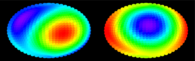
Figure 1: Aithoff-Hammer projections of the front hemisphere $-\pi/2<{\it l}<\pi/2$ of the CMB temperature map in the spin $l=2$ quadrupole (left) and $l=3$ octupole (right) modes. The back side is trivial from the symmetry of the modes.

2.1 A Linear Map

Here we teach ourselves how to factor $l$-pole expansions. The problem of factoring is geometrical and would be much the same for any angular quantity.

If the state $|\psi(l)>$ were an eigenstate of $J_{z}$ with eigenvalue $m^{\prime}$ in the frame where $J_{z}$ is diagonal, we could obtain a relation

$$<m|\,J_{z}|\psi(l)>\,\rightarrow m\,\delta_{mm^{\prime}}.$$

Here $|m>=|l,\,m>$ is a concise notation. Correspondingly, if we rotated the operator $\vec{J}$,

$$\vec{J}\rightarrow\vec{J}(\alpha,\,\beta,\,\gamma)=U_{l}(\alpha,\,\beta,\,\gamma)\vec{J}U_{l}^{\dagger}(\alpha,\,\beta,\,\gamma),$$

then we could determine the same relation for an eigenstate in an arbitrary frame related by Euler angles $\alpha,\,\beta,\,\gamma$. It follows that there is a linear map or “wave function” $\phi_{m}^{k}$ which contains the information on frame-orientation:

$$\phi_{m}^{k}=\frac{1}{\sqrt{l(l+1)}}<m|\,J^{k}|\psi(l)>.$$ (3)

The ranges of indices is $k=1\ldots 3$ and $m=-l\ldots l$. We call this a wave function in analogy with the Bethe-Salpeter wave function, which is the matrix element of the operator creating a quantum state (analogous to $J_{\pm}=J_{x}\pm iJ_{y}$) and a fiducial vacuum state (analogous to $|m=0>$.) We are not doing quantum mechanics and the physical observables exist at the level of this wave function, not the wave function-squared. Most importantly, $\phi_{m}^{k}$ is linear in the data and transforms like a vector in the index $k$ and a rank $l$ tensor in the index $m$.

2.1.1 Completeness

The map to $\phi_{m}^{k}$ is simply a coordinate transformation. Start with $\psi_{m}=<m|\psi>$, of course for fixed $l$. Make

$$\phi_{m}^{k} = \Gamma_{mm^{\prime}}^{k}\psi_{m^{\prime}};$$

$$\Gamma_{mm^{\prime}}^{k} = \frac{1}{\sqrt{l(l+1)}}<m|\,J^{k}\,|m^{\prime}>.$$ (4)

Repeated indices are summed. Since $\phi_{m}^{k}$ has two indices, and $\psi_{m^{\prime}}$ has one index, the transformation is not obviously invertible. But the assignment of indices simply records the division of the space. The inverse of $\Gamma_{mm^{\prime}}^{k}$ exists and is denoted $\Gamma_{k}^{mm^{\prime\prime}}.$ Construct the inverse directly:

$$\Gamma_{k}^{mm^{\prime\prime}}=\frac{1}{\sqrt{l(l+1)}}<m|\,J^{k}\,|m^{\prime\prime}>;$$

$$\Gamma_{k}^{mm^{\prime\prime}}\Gamma_{m^{\prime\prime}m}^{k} = \frac{1}{l(l+1)}<m|\,J^{k}\,|m^{\prime\prime}><m^{\prime\prime}|\,J^{k}\,|m^{\prime}>,$$ (5)

$$= \frac{1}{l(l+1)}<m|\,\vec{J}^{2}\,|m^{\prime}>,$$

$$= \delta_{mm^{\prime}}.$$

Technically $\Gamma_{k}^{mm^{\prime\prime}}$ is a pseudoinverse (Moore-Penrose inverse) for the two indices $m,\,k$ lying on the subspace of fixed $l$. The map to $\phi$ is unitary for each $l$.

2.1.2 Invariantly Preferred Frames

Although $\phi_{m}^{k}$ is neither symmetric nor Hermitian in general, it has an invariantly preferred coordinate frame - in fact, two frames. The frames are found by the singular value decomposition ($svd$)

$$\phi_{m}^{k}=\sum_{\alpha}^{A}\,e_{k}^{\alpha}\Lambda^{\alpha}u_{m}^{{}^{\dagger}\,\alpha}.$$ (6)

The matrix elements $e_{k}^{\alpha}$ and $u_{m}^{\alpha}$ are “unitary” (i.e. orthogonal when real):

$$\sum_{m}\,u_{m}^{\alpha}(u_{m}^{\alpha^{\prime}})^{*}=\delta_{\alpha\alpha^{\prime}};$$ (7)

$$\sum_{k}\,e_{k}^{\alpha}(e_{k}^{\alpha^{\prime}})^{*}=\delta_{\alpha\alpha^{\prime}}.$$ (8)

It follows that in a coordinate system rotated by $e$ on index $k$ and rotated independently by $u^{\dagger}$ on index $m$ the expansion of $\phi_{m}^{k}\rightarrow(\Lambda^{1},\,\Lambda^{2},\ldots\Lambda^{A})$ and diagonal. This is what is meant by “an invariantly preferred coordinate system”. In the preferred coordinates, the frame $e_{k}^{\alpha}\rightarrow\delta_{k\alpha}$, meaning that $e^{1}\rightarrow$ (1, 0, 0 …), and so on. The rest of $\phi_{m}^{\alpha}$ becomes a definition of the particular vector chosen to be a fiducial basis: the case $\phi_{0}^{\alpha}$ is a perfectly adequate “vacuum.” So the meaning of the $svd$ is that we can relate any state by a few invariants and a rotation to an invariantly determined reference frames.

Consistency requires that the number of terms $A$ does not exceed the dimension of the smaller space. For $l=1$ there is a degeneracy and the number of terms $A=2$. In all cases $A\leq 3$. The matrices $u_{m}^{\alpha}$ are not a complete “frame” but have the nature of a coset. The eigenvalues $\Lambda^{\alpha}$ are invariant, real, and by conventions of phase, positive. The $svd$ is the direct generalization to two independent spaces of the usual fact that a Hermitian matrix can be diagonalized with the conjugate coordinate transformations acting on the left and the right. For those with backgrounds only in quark physics, the $svd$ is the procedure to reduce the CKM matrix to its invariant terms and unitarily-related frames.

Degeneracy

If two or more eigenvalues $\Lambda^{\alpha}$ are equal then $\psi$ is invariant under the corresponding orthogonal symmetry. While this is rare, a degeneracy happens to occur in the data at hand, as seen momentarily.

2.1.3 Axial Quantities

Starting from our standard coordinate frame $\{|i>\}$ with names $i$, with $<j|i>=\delta_{ij}$, $<j|3>=(0,\,0,\,1)$, and so on, the three vectors $e_{k}^{1},\,e_{k}^{2},\,e_{k}^{3}$ represent three preferred orthogonal axes in space. Sometimes we will use the notation $\hat{e}^{\alpha}$ for this reason. We assess the importance of these axes by the weights $\Lambda^{\alpha}$. They parametrize the degree of asymmetry. Ordering the eigenvalues from largest to smallest, the first frame element designated by $\alpha=1$ describes a preferred axis. We reiterate that eigenvectors describe an axis, in the meaning of an oriented line in space, not signed-vectors in the sense of having a direction. In detail this comes because the signs of the $e^{a}$ are conventions fixed by the signs of the weights $\Lambda^{\alpha}$. Numerical code can conceal this fact.

2.1.4 The Quadrupole

The quadrupole is very instructive. A quadrupole set of 5 numbers $(q_{-2},\,q_{-1},\,\ldots q_{2})$ is just the relisting in the angular momentum basis of the 5 elements of a traceless symmetric 3$\times$ 3 Cartesian tensor $Q_{ij}$:

$$Q_{ij}=V_{ij}^{m}\psi_{m}(l).$$ (9)

Here $V_{ij}^{m}$ is a unitary set of coefficients to change indices $m$ to indices $ij$.

Such a tensor has an obvious preferred frame in which it is diagonal:

$$Q=\sum_{\alpha}^{3}\,|q^{\alpha}>\Lambda_{Q}^{a}<q^{\alpha}|.$$

How are the obvious frame elements $|q^{\alpha}>$ related to the frame elements $|e^{\alpha}>$ defined by $svd$?

They are the same frame, as evident by symmetry of diagonalizing on the left. The demonstration is awkward and we simply verified the fact with numerical examples.

2.2 Frames Defined by Expectation Value

De Olviera et al (dOZTH)[2] have obtained a special axis for the CMB quadrupole and octupole by the following procedure. Define $\hat{n}=\hat{n}(\theta,\,\phi)$ as a unit vector depending on angular parameters $\theta,\,\phi$. Find the maximum of the quadratic expectation of $(\vec{J}\cdot\hat{n})^{2}$,

$$<\psi(l)|\,(\vec{J}\cdot\hat{n})^{2}\,|\psi(l)>\rightarrow max.$$ (10)

The sign of $\hat{n}$ is, of course, not determined by Eq. 10. dOZTH report finding maximal unit vectors by a numerical search with the 3,145,728 pixel map. Using galactic coordinates and the standard conventions of axes (see Appendix), they find for the quadrupole and octupole:

$$\hat{n}(l=2)=\pm(-0.1145,\,-0.5265,\,0.8424);$$

$$\hat{n}(l=3)=\pm(-0.2578,\,-0.4207,\,0.8698).$$ (11)

We think this is an important result and we will return to it.

Besides one axis of absolute maximum weight, we observe there are always two other $\hat{n}$ per multipole giving local maxima. We see this by writing

$$<\psi(l)|\,(\vec{J}\cdot\hat{n})^{2}\,|\psi(l)>=\hat{n}_{k}K^{kk^{\prime}}\hat{n}_{k};$$

$$K^{kk^{\prime}}=<\psi(l)|\,J^{k}J^{k^{\prime}}\,|\psi(l)>.$$ (12)

Since the commutator of the $J$’s gives no contribution, $K^{kk^{\prime}}$ is symmetric in its indices. By the Rayleigh-Ritz variational theorem $\hat{n}$ will be one of three eigenvectors of $K$ when the expectation is extremized. (There would be $N$ such eigenvectors for $N$ group generators.) That is, the variational problem determines a frame.

Earlier we mentioned that tensor quantities quadratic in the temperature do not have the interpretation of temperature. What is the relation of the quadratically-produced $K^{kk^{\prime}}$ axis and the one from $svd$? It is a matter of suppressing information in $\phi_{m}^{k}$. Consider $\phi_{m}^{k}$ as a matrix $\phi$ with indices $k,\,m.$ Make a Hermitian square matrix that sums over the information in index $m$:

$$\phi\phi^{\dagger} = \sum_{\alpha}\,|e^{\alpha}>(\Lambda^{\alpha})^{2}<e^{\alpha}|;$$

$$<k|\phi\phi^{\dagger}|k^{\prime}> = \sum_{m}<\psi(l)|\,J^{k}|m><m|J^{k^{\prime}}\,|\psi(l)>,$$ (13)

$$= K^{kk^{\prime}}.$$

The $u$-frames disappear in the sum due to unitarity. This is a rather magical version of unitarity, as the coset $u_{m}^{\alpha}$ with $-l<m<l$ indices only just spans the three-dimensional subspace $\alpha=1\ldots 3$ it needs to span. The diagonal frame of $K$ coincides with the diagonal left-frame of $\phi_{m}^{k}$, namely the frame defined by the $e^{\prime}s$. Meanwhile the weights of $K$ are the weights of $\phi$ squared.

We have shown, then, that a potential objection to an axis obtained from one particular method quadratic in the data is not a worry, because it is the same axis inherent linearly in the data. The objection remains true for other methods.

2.3 Our Calculation

We made our calculation (Table 1) for the quadrupole and octupole by making the spin-2 and spin-3 angular momentum matrices and diagonalizing by $svd$. The results are compatible with dOZTH with small differences. We find frame axes with largest eigenvalues:

$$\hat{e}^{(1)}(l=2)=(0.112,\,0.506,\,-0.855);\>\>\>spin-2$$

$$\hat{e}^{(1)}(l=3)=(0.246,\,0.399,\,-0.883).\>\>\>spin-3\$$ (14)

Our sign conventions are fixed by $\Lambda^{\alpha}>0$, which is standard. The eigenvalues and complete frames are listed in Table 1. We checked our result by comparing them to a direct diagonalization of the traceless symmetric Cartesian tensor for spin-2 , and by a third method using Clebsch-Gordan coefficients (see below). We believe the small differences are not significant: $\hat{n}(l=2)\cdot e^{(1)}(l=2)$=0.9996. There will be small differences going from the pixels to the moments, and it is impossible to obtain very high accuracy for an eigenvector by a variational method due to the object function becoming stationary.

What about the eigenvalues? Consulting Table 1, the largest eigenvalue is indeed large, and apparently inconsistent with an uncorrelated isotropic proposal. We will discuss quantifying such features shortly. The octupole’s two “small” eigenvales $\Lambda^{(2)},\,\Lambda^{(3)}$ are nearly degenerate. The frame of the octupole $e_{k}^{\alpha}(l=3)$ is far from isotropic but can be aligned with the other frames with very small changes in the inputs.

spin	$\Lambda^{\alpha}\>\>\>\>\>\>$	$\hat{e}_{1}\>\>\>\>\>\>\>\>\>\>$	$\hat{e}_{2}\>\>\>\>\>\>\>\>\>\>$	$\hat{e}_{3}\>\>\>\>\>\>\>\>\>\>$

l=2	25.95	0.1115	0.5049	-0.8559
	17.70	0.3874	0.771	0.5053
	8.24	0.9151	-0.3880	-0.1095

l=3	47.35	0.2462	0.3992	-0.8831
	21.94	- 0.9383	0.3262	-0.1141
	21.24	0.2425	0.8568	0.4550

Table 1: Cosmic Axial Coincidence of quadrupole and octupole orientation. Top Group: Frame matrix elements from the quadrupole for $e_{k}^{\alpha}(l=2)$ in rows $\alpha=1..3$ and columns $k$=1…3. Bottom Group: Same for the octupole $e_{k}^{\alpha}(l=3)$. The octupole has a nearly perfect degeneracy, allowing the lower two rows to be freely rotated about the $e_{k}^{3}(l=3)$ axis. In that case the two frames nearly coincide.

2.4 Other Methods

We gave thought to the question of uniqueness, because it is tedious to analyze what other axial quantities might be made using higher powers of variables beyond the linear and quadratic constructions discussed so far.

Under the rotation group, the product of two or more representations $|l,\,m>\otimes|l^{\prime},\,m^{\prime}>$ is reduced to a sum of tensors of rank $|J,\,M>$ by the Clebsch-Gordan series or “clebsches”. So if we want a quadrupole in order to make axes, and it must come from from the product of two octupoles (say), then we need the $3\otimes 3\rightarrow 2$ clebsches and it can be worked out. We must distinguish the maps of $|l,\,m>\otimes|l^{\prime},\,m^{\prime}>$ and $|l,\,m>\otimes<^{\prime},\,m^{\prime}|$, of course.

2.4.1 Products of $l\otimes l^{*}$

The clebsches for real symmetric projections $l\otimes l^{*}\rightarrow 1$ vanish, just as the expectation $<\vec{J}>=0$ indicates. In fact $\vec{J}$ is just the operator of clebsches to make spin-1 from such products. We do not seek a vector, but a symmetric rank-2 tensor to make axes. Evidently $C^{kk^{\prime}}(2)=<J^{k}J^{k^{\prime}}-\frac{1}{3}\vec{J}^{2}\delta^{kk^{\prime}}>$ is the appropriate map from $l\otimes l^{*}\rightarrow 2$, as just discussed. The unit operator $\frac{1}{3}\vec{J}^{2}\delta_{kk^{\prime}}$ added to make a traceless irreducible representation does not change the eigenvectors, but does remove one independent eigenvalue. The connection with clebsches makes the procedure of dOZTH less miraculous and shows that the $svd$ frames, then, coincide with a Clebsh-Gordan series of squaring the data, projecting down into spin 2, and finding the preferred frame of the product.

Although the result is trivial we checked our calculation of $\hat{n}_{2},\hat{n}_{3}$ a third way by generating it by the CG series for $l\otimes l^{*}$.

2.4.2 Products of $l\otimes l$

What about the clebsch projections of products without complex conjugation? One finds that $l\otimes l\rightarrow 1$ and $l\otimes l\rightarrow 2$, and so on, are non-zero, and perfectly valid complex quantities. If one’s experience is limited to neutrino physics, these are like “Majorana” masses which take the non-conjugated products of the Lorentz group and make a scalar. From the $svd$ decomposition one can gain insight on what they mean. Form the outer product

$$\phi_{k}^{m}\phi_{k^{\prime}}^{m^{\prime}}=\sum_{\alpha,\beta}\,\,e_{k}^{\alpha}e_{k^{\prime}}^{\beta}\Lambda^{\alpha}\Lambda^{\beta}u_{m}^{{}^{\dagger}\,\alpha}u_{m^{\prime}}^{{}^{\dagger}\,\beta}$$ (15)

Now a clebsch series to get spin-$J$ will project this by contracting with a matrix $C_{mm^{\prime}}^{J}$. The overall form resulting is

$$C_{mm^{\prime}}^{J}\phi_{k}^{m}\phi_{k^{\prime}}^{m^{\prime}}=e_{k}^{\alpha}W_{J}^{\alpha\beta}e_{k^{\prime}}^{\beta}.$$ (16)

This is far from a diagonal form as there is no “dagger” on either symbol $e$. The function of $W_{J}^{\alpha\beta}$ is to mix the information in the $u_{m}^{l}$ not transforming like vectors until spin-J comes out of the mix.

While spin-2 can be made, it is complex, and it is hard to get excited about an $m=1$ (say) term made from the product of $l=97,\,m=93$ and $l=97,\,m=94,\,m=92$ that never existed before the data was squared. We do not pursue this or further products, given the invertibility of $\phi_{m}^{k}$ (Eq. 5) that tells us it is complete.

3 Cosmic Axial Coincidences

We constructed symmetry methods to pursue a higher goal than classification. We turn to several striking coincidences among the CMB[2] and other axial quantities, all obtained from radiation propagating on cosmological distances. The coincidences pose a significant puzzle.

First, the quadrupole and octupole axes coincide closely with each other, and with a well-known third axis $\hat{e}_{dipole}^{1}$ pointed toward Virgo. The relations are:

$$\hat{e}_{dipole}^{1}\cdot\hat{e}_{quad}^{1}=0.980$$

$$\hat{e}_{quad}^{1}\cdot\hat{e}_{octo}^{1}=0.985$$

$$\hat{e}_{octo}^{1}\cdot\hat{e}_{dipole}^{1}=0.939.$$ (17)

Compare these to the default symmetry-based hypothesis that each vector is uncorrelated with the others and distributed isotropically. This happens to be the basic Big Bang ($bBB$) null, and no further assumptions are needed to employ it. The coincidence of three vectors in nearly the same direction is not at all expected.

3.1 Coincidence with Independent Radio Frequency Observables

In Ref. [3] an axis of anisotropy for radiation propagating on cosmological scales was reported: in galactic coordinates the axis is found to be

$$\hat{s}_{JR}=(-0.0927,0.4616,-0.8822).$$

This axis coincides with the direction of Virgo. It is very remarkable that this axis coincides with axial parameters from the CMB.

The result came from a test of propagation isotropy. The paper examined statistics of offset angles of radio galaxy symmetry axes relative to their average polarization angles for 332 sources[3]. The polarization offsets are variables understood to be independent of intervening magnetic field. Faraday rotation measures $RM$ are removed source-by-source in linear fits to wavelength dependence. Further discussion is given in the Section on Mechanisms. Now there are four coincident axes.

3.2 Coincidence with Optical Frequency Observable

In Refs. [4] Hutsemékers observed that optical polarization data from cosmologically distant and widely separated quasars indicate an improbable degree of coherence. The alignment of polarizations on a curved manifold (the sky) is tricky to assess and certain statistics invariant under coordinate changes are needed. In Ref. [5] invariant statistics were constructed using parallel-transport. The facts of unusual coherence were confirmed, and moreover a significant clustering of polarization coherence in large patches in the sky was observed.

The axis of correlation obtained from a fit is

$$\hat{s}_{Hut}=(0.0344,0.4844,-0.8741)\ ,$$

in galactic coordinates. The axis given above has been obtained by imposing the cut on the degree of polarization $p\leq 2$ %. This cut gave the largest optical polarization alignment effect [5]. The axis obtained by the full data agrees within errors. This axis coincides with the direction of Virgo.

Now there are five coincident axes.

3.3 CMB Polarization Observables

COBE led the way in measuring moments of the temperature map beyond the dipole. WMAP [6] observations yield highly detailed information on CMB polarizations for the first time. Among the features not predicted by the $bBB$ is a highly significant cross-correlation of the temperature and degree of polarization (Stoke’s $Q$) across very large angular scales.

WMAP uses an invariant polarization statistic equivalent to parallel transport[5]. The observed correlations are inconsistent with the $bBB$ predictions of uncorrelated isotropy on such scales. A subsequent re-ionizing phase has been proposed [7] to explain them.

We remarked earlier that the conventional $bBB$ has been ruled out. Insertion of a new hypothesis to explain the polarization correlation justifies that remark. Meanwhile we see no reason, even under the burden of the new hypothesis, for the polarization quantities to have any preferred axial character.

For some reason WMAP has not released polarization data, as far as we know. We predict that WMAP may see an increased degree of polarization in the direction of Virgo, ordiametrically opposite. One cannot deduce this from the correlation itself. We simply see a pattern here. Our prediction is empirical and based on the fact that the CMB already points to Virgo in the dipole, quadrupole, and octupole axes. Correlation with Virgo would simply be more of the Virgo Alignment.

3.3.1 Directionality

Given the opportunity to speculate, the pattern of data also indicates to us that CMB-derived polarizations should be aligned towards Virgo, along the plane found by Hutsemékers. Like the others, this deduction does not follow from the correlations published. It follows on the basis of inspecting patterns in data without imposing too many prior assumptions.

3.4 Quantification with Bayesian Priors

Here we consider the statistical significance of some coincidences.

The null is uncorrelated isotropy. The usual test of the null is

$$P(null\,|\,data)=\frac{P(data\,|\,null)P(null)}{P(data)}.$$ (18)

The probability of two axes $\hat{e}_{A},\,\hat{e}_{B}$ coinciding from the null to a degree equal or better than the data is the area of the largest spherical cap touching them divided by $2\pi$:

$$P(e_{A}\cdot\hat{e}_{B}\,|\,null)=1-|e_{A}\cdot\hat{e}_{B}|.$$ (19)

The probability of three coincidences is the product:

$$P(e_{A}\cdot\hat{e}_{B},\,e_{B}\cdot\hat{e}_{C}\,|\,null)=(\,1-|e_{A}\cdot\hat{e}_{B}|\,)(\,1-|e_{B}\cdot\hat{e}_{C}|)\,).$$ (20)

We summarize the numerical value of pairwise probabilities in Table 2.

Figure 2: Updated probabilities disfavoring the conventional big-bang isotropic null hypothesis. The solid curve shows the calculated probability of the hypothesis $log_{10}(\,P(null\,|\,3\,axes)\,)$ after seeing the coincidence of dipole, quadrupole, and octupole axes (only) as a function of prior prejudice $P(null)$. The dashed curve shows $log_{10}(1-P(null))$, an estimator of the probability of the alternate hypothesis.

Continuing, we need $P(null)$, which comes from outside, and is difficult to settle. There may be an impulse to revert to large $l$ correlations and declare $P(null)=1$. But large $l\geq 100$ correlations made in a manifestly isotropic way add no independent information to the problem at hand. The things commonly predicted, namely magnitudes of the low $l$ moments, don’t agree with the standard null. We find there is no good value for $P(null)$.

For argument let $P(null)=0.999$ simply because we can say it is so. We need an alternate hypothesis $P(axes)$ to proceed. This will be the hypothesis that axes are well-correlated. It may appear retrospective, but follows from the non-CMB data (Section 3). Quibbling is pointless because in a two-option contest $P(axes)=1-P(null)=0.001<<1$ is very unlikely anyway. By definition $P(e_{A}\cdot\hat{e}_{B},\,e_{B}\cdot\hat{e}_{C})\sim 1$ if axes tend to be correlated. So long as $P(axes)$ is small enough the details of $P(axes)$ will not change the evaluation of the data. Now calculate by Bayes Theorem: after seeing the coincidence of the dipole, quadrupole, and octupole axes, the updated probability of the null:

$$P(null\,|3\,axes)\sim\frac{P(3\,axes\,|\,null)P(null)}{P(3\,axes\,|\,null)P(null)+P(3\,axes\,|\,cor)P(cor)},$$

$$=\frac{0.02\times 0.015\times 0.999\,}{0.02\times 0.015\times 0.999\,+1\times 0.001}$$

$$=0.23.$$ (21)

The null survives because we used such a strong prejudice favoring the $bBB$. Yet if one had expressed less confidence, say $P(null)=0.990$, the result would have changed, yielding $P(null\,|3\,axes)\rightarrow 0.029,$ and ruling out the null. As a crisp summary, the null is ruled out with $97.1\%$ confidence level, or indeed much more, unless one’s prior prejudice favoring it is $99.0\%$ or higher. For convenience we show parametrically the data-driven confidence level in the null and the alternative hypothesis, as a function of initial prejudice (Fig. 2).

	dipole	quad	octo	JR	Hutsemékers
dipole		0.020	0.061	0.042	0.024
quad			0.015	0.023	0.004
octo				0.059	0.026
JR					0.008

Table 2: Probabilities as P-values $P$, for the axis coincidence listed to equal or exceed that seen in the data under an uncorrelated isotropic distribution. By ordinary convention $1-P$ is the confidence level that the uncorrelated isotropic hypothesis is false.

3.4.1 Other Arguments

It is interesting how a coincidence can be explained away by a Bayesian re-arrangement of logic. Assuming from the boost interpretation that the dipole axis “can be of no cosmological significance” (goes the argument), we remove one vector freedom in the product of three possible probabilities. Then only two things coincide, and the astonishing improbability of the coincidence is reduced to a merely alarming value.

Is this a swindle? It depends. Nobody can argue with a Bayesian argument because the proponent who defines the priors may define their own priors. The simpler and more direct expression of prior prejudice will hold that all the low $l$ moments have no (or little) cosmological significance. In that case, nobody should not have even looked at (let alone paid millions for) the data!

There is a Bayesian response: let $P(junk)$ be the probability that low-$l$ is junk. “Cosmic variance”, in the assertion that the fluctuations of a few degrees of freedom tend to equal their value, is for us on the logical track proportional to $P(junk)$. In that case the comparison of three axes would not be meaningful, except to update prior beliefs in $P(junk)$.

We are not ready to assume that the bulk of the data in a large-scale sense is just extremely expensive junk. Given the cost and the potential importance of the decision we feel it would be highly irresponsible to do so. The logical chain proportional to $1-P(junk)$ is the chain capable of testing the null. The smallness of $1-P(junk)$ is the entrance price for asking challenging questions. One is not supposed to assess the entrance fee a second time when something surprising is actually found.

Under the original hypothesis, and not adding further qualifications, the conditional probability of coincidence $P(\hat{n}_{1},\,\hat{n}_{2},\hat{n}_{3},|\,bBB)$ of three axes is an extremely unlikely occurence.

4 Mechanisms

The optical properties of cosmological propagation are not directly connected to the Big Bang by general principles and need not have significant other consequences.

It is also not necessary to have a mechanism to recognize regularities in data. Proposing mechanisms is helpful toward suggesting interpretations and further tests.

Here we review information on the non-CMB axes and then turn to potential mechanisms.

4.1 Faraday Rotation Data

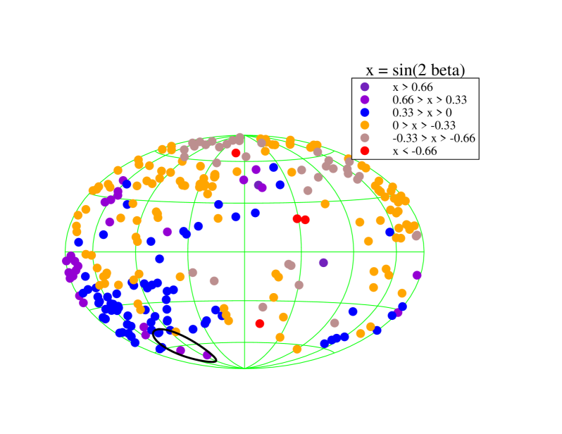
Figure 3: Covariant polarization offset statistics $x=sin(2\beta)$, where $\beta$ is the offset angle between galaxy symmetry axes and polarization planes, for 265 radio galaxy sources mentioned in the text. The prefered axis $(l=101.36^{o}\pm 15^{o},\ b=-61.91^{o}\pm 15^{o})$ is shown as a black cross. Axial clustering is readily visible to the eye.

There is a long history of observation of anisotropy at GHz frequencies. Controversies have been generated by discordant signals in statistics initially supposed to represent the same phenomena. Over a period of years, the discrepancies were traced to different symmetries in the quantities being reported. There is a consistent signal in odd-parity statistics sensitive to a direction of polarization rotation.

Birch[8] observed patterns in data empirically. Kendall and Young[9] confirmed Birch with a likelihood analysis. Bietenholz and Kronberg[10] verified Birch’s results, and confirmed a statistically significant effect in a larger data set. They dismissed the claim by turning to a statistic of even parity symmetry developed by the statisticians Jupp and Mardia[11]. Nodland and Ralston [12] reported a redshift-dependent odd-parity correlation in a set of 160 sources with known redshifts. These data indicated correlations of offsets with an axis oriented toward Virgo. Carrol and Field [13] dismissed the signal using RMS angle measures that are coordinate-dependent[14]. Eisenstein and Bunn re-plotted the data on the basis of even parity and dismissed the signal by eye [15, 16]. Loredo et al[17] found no signal in an invariant statistic of even parity.

A symmetry analysis[14] showed that the Jupp-Mardia ($JM$) statistics come in even and odd-parity classes. Ref. [3] reported axial correlations obtained from a larger set of 332 radio galaxies. Integrating over redshifts made statistics more robust and increased the size of available data. Both coordinate-free odd-parity $JM$ statistics and likelihood analysis showed a strong signal. The case of highest significance, about 3.5 $\sigma$, was found using an $RM$ cut parameter. The cut is $(RM-\overline{RM})\geq 6\ rad/m^{2}$, where $\overline{RM}$ is the mean value of $RM$ in the sample. A related study [18] yield axes consistent with the axis of Eq. 3.1 within errors. In fig. 3 we show the scatter plot of $\sin(2\beta)$ for the 265 source data sample considered in Ref. [3] after imposing the cut $(RM-\overline{RM})\geq 6\ rad/m^{2}$. Here $\beta$ is the angle between the observation polarization angle, after taking out the effect of the Faraday Rotation, and the galaxy orientation angle. The figure shows the averaged value of the variable $x=\sin(2\beta)$ at each position, where the average is taken over the nearest neighbours which satisfy $\hat{r}_{1}\cdot\hat{r}_{2}>0.95$. Here $\hat{r}_{1}$ and $\hat{r}_{2}$ refer to the angular positions of the two sources.

The mechanism for these correlations remains unknown. The population in $RM$ is peculiar, with a tall central spike and long tails. The population and correlations might suggest an artifact of the data-fitting procedure, which used the faulty concept of RMS angle. However re-fitting the original data to obtain $RM$ and offset values by an invariant statistical method [19] did not change the conclusions significantly.

4.1.1 Plasma Explanations?

Perhaps Faraday rotation results could be explained away by the ineluctable peculiarities of plasma electrodynamics. One study of different statistics taken at higher frequencies saw no signal in a selection of polarization and jet axes. [20]

Faraday rotation depends on the longitudinal component $B_{||}$ of the magnetic field, which must certainly fluctuate over cosmological distances. However adiabatic propagation models traditionally used break down at field direction reversals[21] $B_{||}\rightarrow 0$. This conventional physics was not included in the astronomical $RM$ analysis, and flips polarizations. It might be a candidate for explanation. Large angular scale correlations in galactic or cosmological magnetic fields, however, would be required for this mechanism to explain the Faraday rotation data. Galactic fields were always a concern for $RM$ measurements and were thought to be understood. We continue along these lines in the subsection on Foreground Mechanisms below.

Cosmological magnetic fields of dipole, quadrupole or octupole character have always formed a highly virulent threat to Big Bang dynamics. Little reliable information exists about cosmological magnetic fields[22], and data at frequencies dominated by Faraday rotation poses inherent difficulties of interpretation.

The CMB data, with frequency much larger than Faraday rotation measurements, are thought to be comparatively free of such effects. Compensations are made for the effects of the ionosphere and galaxy. Under the standard hypotheses, the CMB measurements form an independent observable which should not be related to Faraday rotation data.

4.2 Optical Data

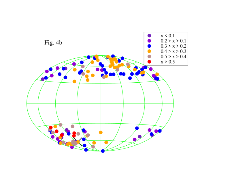
Figure 4: Optical polarization alignment observed by Hutsemékers [4] in (a) equatorial and (b) galactic coordinates. Here $x$ refers to the correlation statistic, defined in text, with the number of nearest neighbours chosen to be 28. The data within the galactic plane was deleted [4] in order to minimize the effect of galactic extinction. Effects of population are taken into account in the construction of the prefered axis, shown as a black cross at $l=85.94^{o},\ b=-60.94^{o}$. Axial clustering is readily visible to the eye.

The interpretation of Hutsemékers result and subsequent verification is complicated by the possible processes affecting optical polarization along the trajectory. The primary model to change the degree of polarization is preferential extinction by dust. However any correlation of dust across vast cosmological distances would be as alarming as a correlation of magnetic fields or the CMB radio spectrum.

Peculiarly, the data fraction of smallest polarizations has the highest significance. In Fig. 4 we show the distribution of correlation statistic $x=S_{D}^{p}$, defined in Ref. [5], for the 146 source data sample after imposing the cut $p\leq 2$ %. The statistic $S_{D}^{p}$ is the mean value of the dispersion over the entire sample. A measure of the dispersion at each point is obtained by maximizing the function,

$$d_{i}(\theta)={1\over n_{v}}\sum_{k=1}^{n_{v}}\cos\left[2\theta-2\left(\theta_{k}+\Delta_{k\rightarrow i}\right)\right]\ ,$$

with respect to the angle $\theta$. Here $(\theta_{k}+\Delta_{k\rightarrow i})$ is the polarization at the position $k$ after parallel transport to position $i$ along the great circle joining these two points. The symbol $n_{v}$ is the number of nearest neighbours. Fig. 4 uses $n_{v}=28$, a value giving the strongest signal of alignment.

Although thought to be under control, we cannot rule out foreground effects here and refer to the subsection on Foreground Mechanisms below.

4.3 Mechanisms

We considered the following mechanisms:

$\bullet$ Foreground Mechanisms: All of the data cited has potential weaknesses in depending on models of the foreground, and in particular, the effects of our Galaxy.

A great deal of ingenious technical effort has gone into taking this into account without inducing biases. It is unlikely that statistical procedural errors exist. Nevertheless there may be systematic physical processes not taken into account in current CMB foreground subtraction, which cause an alignment with features of our Galaxy. In the spirit of current CMB fits, there is reason to believe that free adjustment of many galactic magnetic field and optical extinction parameters might explain not only the CMB data but also the non-CMB correlations.

It is somewhat hard to see how substantial foreground corrections that might make axial alignment correlations go away would not change CMB data and preserve its current interpretation as a pristine record of the early universe.

$\bullet$ Metric Mechanisms: The propagation of polarizations is an old subject in General Relativity [23]. In the freely-falling frame where the metric is trivial, general covariance says that the two polarizations propagate equally in Maxwell’s theory, and will preserve the state and direction of polarization. This is due to a symmetry of duality that the metric theory happens to preserve. Large polarization effects would need large curvature effects that are not observed. Given present information and beliefs about the large-scale flatness of the Universe, we do not know of a way for the large effects in the polarization data cited to be explained.

$\bullet$ Magnetic Fields in the Early Universe: The scaling laws of magnetic fields are such that their imprint on the present Universe can be hard to trace. However large-scale magnetic fields clearly could affect the $CMB$. We cannot review all the work done in this regard: It is simply hard to see how magnetic fields at small redshift could conspire in conventional physics to explain the Faraday offset anisotropies, and it seems impossible to explain the Hutsemékers data.

$\bullet$ Dark Energy: If dark energy is due to a scalar field there is a simple generic mechanism to produce surprising optical effects that do not necessarily disturb the other predictions of $bBB$ models. Since we have not seen this discussed elsewhere, we summarize it in broad terms, referring the reader to a companion paper[24].

During the process of expansion and decoupling, the photon field changes dramatically over a wider range than any other particle. The change occurs in the photon mass. The photon is massless en vacuo due to the local nature of the theory and gauge invariance. The photon is not massless in general, but propagates with a mass $m_{p}^{2}$ given by the “plasma frequency” $\omega_{p}^{2}=m_{p}^{2}c^{4}$. The usual non-relativistic formula for the plasma frequency is

$$\omega_{p}^{2}=\frac{e^{2}n}{4\pi m_{e}},$$

where $-e$ is the electron’s charge, $n$ is the density of light (electron) carriers, and $m_{e}$ is the electron mass. The dispersion relation en plasmo is

$$\omega^{2}-c^{2}\vec{k}^{2}=m_{p}^{2}c^{4}.$$ (22)

Any scalar field $\phi$ coupling to the electromagnetic field strength $F^{\mu\nu}$ will mix resonantly in a background magnetic field when the scalar mass is same as the photon mass. A typical Action is

$$S=\int d^{4}x\sqrt{g}\,\,\left(\frac{-1}{4}F^{\mu\nu}F_{\mu\nu}+g\phi\epsilon_{\mu\nu\alpha\beta}F^{\mu\nu}F^{\alpha\beta}\right),$$ (23)

which suffices to break duality symmetry. Parameter $g$ is a dimensionful coupling constant that can be of exceedingly small size. The physical consequences of the mixing of this scalar field with photons has been studied by several authors [25]. Since the plasma frequency and the scalar mass are independent, and of different scaling characteristics in general, it is hard to avoid scale-crossing. In particular, driving the photon mass to zero crosses every conceivable scale at least once, to say nothing about re-ionization phases. Once duality symmetry is broken, polarization can be spontaneously generated and also rotated under propagation.

No fundamental coupling is required because radiative corrections will generate all couplings allowed by symmetry. The existence of a scalar field –that is, dark energy – is itself sufficient to guarantee that the optical properties of propagation over vast distances and times will not be those of the usual theory. Of course, the organization of dark energy over huge scales is something that cannot be determined in advance. Models such as quintessence hardly encompass the possibilities.

The observation of propagation anomalies is in fact a highly conservative prediction of the current framework of cosmology, without requiring new hypotheses. While constantly cited, the data has ruled out Einstein’s early cosmological constant, the dark action

$$S_{dark}=\int d^{4}x\,\sqrt{g}\,\Lambda.$$

Instead it is necessary to have $\Lambda\rightarrow\Lambda(\vec{x},\,t)$. Now it would violate basic consistency requirements, such as causality, if what is currently meant by $\Lambda(\vec{x},\,t)$ is not associated with the modes of a field. We believe that what is meant by $\Lambda(\vec{x},\,t)$ is at least as dynamical as a field even more than we believe in $\Lambda(\vec{x},\,t)$

Unfortunately the current state of development of theory cannot relate any particular field to any measurement to $\Lambda(\vec{x},\,t)$. One wonders why it is so important. Meanwhile ordinary perturbative methods can relate any field through radiative corrections to an action such as Eq. 23. Thus propagation anomalies may be an effective probe of dark energy, as compared to the rather indirect coupling to gravity via an energy-momentum tensor. We reiterate that light propagation may yield a productive way to look for the effects of dark energy.

$\bullet$ Dark Energy Plus Magnetic Fields

Given that a resonant interaction inevitably occurs between dark energy and electrodynamics, we have to admit ignorance on the potential outcomes in terms of large scale magnetic fields. This is an extremely interesting dynamical problem. The interactions of magnetic fields are not expected to retain isotropy in all features of an expanding Universe. Futher study along these directions seems justified.

5 Concluding Remarks

There is nothing to fault in the beautiful technology bringing moments of the CMB well above $l>100$. Yet the small moments are problematic. The Virgo alignment appears to contradict the standard picture.

We believe that the tests possible in the near future and longer term hinge on polarization quantities. Perhaps the best way to search for dark energy is with light. WMAP may be poised to make a major discovery that goes far beyond the verification of the models of previous generations.

6 Appendix: Conventions

Here we collect details of conventions and procedures.

For spin $l$ we define operators

$$J_{z}=(-l,\,-l+1,\,...l-1,\,l)\>\>(diagonal),$$

and we enter multipole moments as column vectors in the same convention. We define

$$J_{x}=U(0,\,-\pi/2,\,0)J_{z}U^{\dagger}(0,\,-\pi/2,\,0)\ ,$$

where the matrix elements of $U(0,\,\beta,\,0)_{mm^{\prime}}=d_{mm^{\prime}}^{l}(\beta)$ are the Wigner $d$-matrices with the standard phase conventions. Finally,

$$J_{y}=-i\ [J_{z},\,J_{x}\ ].$$

The Hutsemékers axis is obtained as follows. Let $\hat{n}_{i}$ be the unit vector coordinates of the $i$th source on the sky in galactic coordinates. Construct a two point comparison between the $i$ and $j$ polarization, given by

$$C(\hat{n}_{i},\hat{n}_{j})=\cos[\,2\theta_{i}-2(\theta_{j}+\Delta_{j\rightarrow i})]\ ,$$

where $(\theta_{j}+\Delta_{j\rightarrow i})$ is the polarization angle obtained after parallel transport of the polarization plane at position $j$ to the position $i$ along the great circle connecting these two points. Construct the correlation tensor $T^{kk^{\prime}}$,

$$T^{kk^{\prime}}=\sum_{i,j}\hat{n}_{i}^{k}\hat{n}_{j}^{(k^{\prime})}C(\hat{n}_{i},\,\hat{n}_{j})$$

By construction $T\rightarrow 0$ in a population of uncorrelated polarizations and positions. Make the matrix

$$S=M^{-1/2}TM^{-1/2}$$

where $M$ is the matrix of sky locations

$$M^{kk^{\prime}}=\sum_{i}\hat{n}_{i}^{k}\hat{n}_{i}^{k^{\prime}}\ .$$

By construction $S\rightarrow<p>1$ in an isotropic sample with a net polarization parameter $<p>$, so that $S\rightarrow 0$ in the null. The Hutsemékers axis is the eigenvector of $S$ with the largest eigenvalue.

Acknowledgements

Work supported in part under Department of Energy grant number DE-FG02-04ER41308.

References

- [1] G. Efstathiou, MNRAS 346, L26 (2003), astro-ph/0306431; E. Gaztanaga, J. Wagg, T. Multamaki, A. Montana and D. H. Hughes, MNRAS 346, 47 (2003), astro-ph/0304178; C. R. Contaldi, M. Peloso, L. Kofman and A. Linde, JCAP 0307, 002 (2003), astro-ph/0303636; J. M. Cline, P. Crotty and J. Lesgourgues, JCAP 0309, 010 (2003), astro-ph/0304558; M. H. Kesden, M. Kamionkowski and A. Cooray, Phys. Rev. Lett. 91, 221302 (2003), astro-ph/0306597; H. K. Eriksen et al, ApJ 605, 14 (2004), astro-ph/0307507.
- [2] A. de Oliveira-Costa, M. Tegmark, M. Zaldarriaga and A. Hamilton, Phys. Rev. D 69, 063516 (2004), astro-ph/0307282.
- [3] P. Jain and J. P. Ralston, Mod. Phys. Lett. A14, 417 (1999).
- [4] D. Hutsemékers, A & A 332, 41 (1998); D. Hutsemékers and H. Lamy, A & A, 367, 381 (2001).
- [5] P. Jain, G. Narain and S. Sarala, MNRAS 347, 394 (2004), astro-ph/0301530.
- [6] A. Kogut et al, Astrophys. J. Suppl. 148, 161 (2003).
- [7] A. Kogut et al., ApJ Suppl. 148, 161 (2003); astro-ph/0302213.
- [8] P. Birch, Nature, 298, 451 (1982).
- [9] D. G. Kendall and A. G. Young, MNRAS, 207, 637 (1984).
- [10] M. F. Bietenholz and P. P. Kronberg, ApJ, 287, L1-L2 (1984).
- [11] P. E. Jupp and K. V. Mardia, Biometrika 67, 163 (1980).
- [12] B. Nodland and J. P. Ralston, Phys. Rev. Lett. 78 (1997), 3043.
- [13] S. M. Carroll and G. B. Field, Phys. Rev. Lett. 79, (1997), 2934.
- [14] J. P. Ralston and P. Jain, Int. J. Mod. Phys. D 8, 537 (1999), astro-ph/9809282.
- [15] D. J. Eisenstein and E. F. Bunn, Phys. Rev. Lett. 79, 1957 (1997), astro-ph/9704247.
- [16] B. Nodland and J. P. Ralston, Phys. Rev. Lett. 79, 1958 (1997), astro-ph/9705190.
- [17] T. J. Loredo, E. E. Flanagan and I. M. Wasserman, Phys. Rev. D 56, (1997), 7057.
- [18] P. Jain and S. Sarala, astro-ph/0309776.
- [19] S. Sarala and P. Jain , MNRAS 328, 623 (2001), astro-ph/0007251
- [20] J. F. C. Wardle, R. A. Perley and M. H. Cohen, Phys. Rev. Lett. 79, 1801 (1997), astro-ph/9705142.
- [21] J. P. Ralston, P. Jain and B. Nodland, Phys. Rev. Lett. 81, (1998), 26.
- [22] Ya. B. Zeldovich, A. A. Ruzmaikin and D. D. Sokoloff, Magnetic fields in Astrophysics (Gordon and Breach Science Publishers, 1983).
- [23] W.-T. Ni, Phys. Rev. Lett. 38, 301 (1977); M. Sachs, General Relativity and Matter (Reidel, 1982); M. Sachs, Nuovo Cimento 111A, 611 (1997); C. Wolf, Phys. Lett. A 132, 151 (1988); ibid 145, 413 (1990); R. B. Mann, J. W. Moffat, and J. H. Palmer, ibid 62, 2765 (1989); R. B. Mann and J. W. Moffat, Can. J. Phys. 59 1730 (1981); D. V. Ahluwalia and T. Goldman, Mod. Phys. Lett. A 28, 2623 (1993); C. M. Will, Phys. Rev. Lett. 62, 369 (1989); Y. N. Obukhov, ”Colloquium on Cosmic Rotation”, Eds M. Scherfner, T. Chrobok and M. Shefaat (Wissenschaft und Technik Verlag: Berlin, 2000) pp. 23-96; J. P. Ralston, Phys. Rev. D 51, 2018 (1995).
- [24] P. Jain and J. P. Ralston, in preparation.
- [25] D. Harari and P. Sikivie, Phys. Lett. B 289, 67 (1992); G. Raffelt and L. Stodolsky, Phys. Rev. D 37, 1237 (1988); L. Maiani, R. Petronzio and E. Zavattini, Phys. Lett. B 175, 359 (1986); E. D. Carlson and W. D. Garretson, Phys. Lett. B 336,431 (1994); P. Jain, S. Panda and S. Sarala, Phys. Rev. D 66, 085007 (2002).