Does Magnetic Levitation or Suspension Define the Masses of Forming Stars?

Abstract

We investigate whether magnetic tension can define the masses of forming stars by holding up the subcritical envelope of a molecular cloud that suffers gravitational collapse of its supercritical core. We perform an equilibrium analysis of the initial and final states assuming perfect field freezing, no rotation, isothermality, and a completely flattened configuration. The sheet geometry allows us to separate the magnetic tension into a qlevitation associated with the split monopole formed by the trapped flux of the central star and a suspension associated with curved field lines that thread the static pseudodisk and envelope of material external to the star. We find solutions where the eigenvalue for the stellar mass is a fixed multiple of the initial core mass of the cloud. We verify the analytically derived result by an explicit numerical simulation of a closely related 3-D axisymmetric system. However, with field freezing, the implied surface magnetic fields much exceed measured values for young stars. If the pinch by the central split monopole were to be eliminated by magnetic reconnection, then magnetic suspension alone cannot keep the subcritical envelope (i.e., the entire model cloud) from falling onto the star. We argue that this answer has general validity, even if the initial state lacked any kind of symmetry, possessed rotation, and had a substantial level of turbulence. These findings strongly support a picture for the halt of infall that invokes dynamic levitation by YSO winds and jets, but the breakdown of ideal magnetohydrodynamics is required to allow the appearance in the problem of a rapidly rotating, centrifugally supported disk. We use these results to calculate the initial mass function and star formation efficiency for the distributed and clustered modes of star formation.

1 Introduction

Despite the empirical evidence for the formation of stars under a wide variety of physical conditions in the cosmos, and despite more than a half-century of theoretical study, the question of what determines the masses of forming stars from gravitational collapse in large interstellar clouds remains an open one. Ideas range from hierarchical, opacity-limited, thermal fragmentation (Hoyle 1953, Lynden-Bell 1973, Rees 1976, Silk 1977, Bodenheimer 1978, Zinnecker 1984), to magnetically-limited fragmentation (Mestel 1965, 1985), to turbulence-induced fragmentation (Scalo 1985,1990; Larson 1995; Elmegreen & Efremov 1997; Truelove et al. 1998; Elmegreen 2002; Falgarone 2002; Klein et al. 2003), to wind-limited mass infall (Shu & Terebey 1984, Shu et al. 2000).

Shu (1977) pointed out the intrinsic difficulty of defining starlike masses in a large, unmagnetized, isothermal cloud that starts in equilibrium or near-equilibrium and is not bounded by an artificial surface pressure. He commented on the difficulty of fragmentation in such an environment, where the condition of equilibrium of the initial state and the steep velocity gradients of the subsequent inside-out collapse effectively prevent gravitational fragmentation of the type originally contemplated by Hoyle from taking place (see also the debate between Hunter 1967 and Layzer 1964). These comments were subsequently given added force in numerous numerical simulations (see, e.g., Tohline 1980, 1981; Truelove et al. 1998).

Mestel (1965, 1985; see also Nakano & Nakamura 1978) made a crucial distinction between clouds that have dimensionless mass-to-flux ratios greater than unity (supercritical – capable of gravitational collapse), and less than unity (subcritical – incapable of gravitational collapse). He argued that spherical magnetized clouds which are marginally supercritical cannot fragment gravitationally because any spherical subpiece will be subcritical. He speculated, however, that supercritical isothermal clouds that collapse coherently to highly flattened states can fragment into supercritical pieces, each with size comparable to the vertical scale height. These pieces might correspond to stellar masses. Shu & Li (1997) cast doubt on this scenario in the case when field freezing may be assumed and the initial state corresponds again to a state of initial force balance with a significant density and field stratification. Self-similar, inside-out, collapses in such circumstances do indeed show the anticipated flattening, but the dynamically infalling pseudo-disks that result exhibit no tendency to fragment gravitationally. They are prone to other kinds of numerical and perhaps physical instabilities in the presence of non-ideal magnetohydrodynamic (MHD) effects (Allen, Shu, & Li 2003; Allen, Li, & Shu 2003). Indeed, to our knowledge, no reliable numerical simulation of initial non-uniform states of isothermal equilibria, with or without magnetization, has ever been able to demonstrate fragmentation in the subsequent collapse.

Truelove et al. (1998) and Klein et al. (2003) find fragmentation possible in unmagnetized clouds that start with substantial supersonic turbulence. However, the entire self-gravitating cloud cannot resist being turned into stars in the presence of strong shock dissipation (see, e.g., Klessen 2001). This then introduces a problem why such clouds are around today in a universe whose age is many dynamical crossings of molecular clouds (Zuckerman & Evans 1974). Scenarios have been proposed where the star formation occurring in molecular clouds on all scales occupies only one dynamical crossing time before being dispersed (Elmegreen 2000, Hartmann 2003). But given the known overall inefficiency of star formation, these proposals then need to elucidate how the small fraction of cloud matter that came to have star-formation capability arrived at the critical state, and how the vast bulk of the molecular cloud material avoids gravitational collapse and fragmentation.

The problem of rapid turbulent dissipation persists even in the presence of magnetization (Heitsch, MacLow, & Klessen 2001; Ostriker, Stone, & Gammie 2001), unless the magnetization is so strong as to make the clouds subcritical, in which case neither runaway gravitational collapse nor gravitational fragmentation will occur, even if the turbulence dissipates completely. In any case, in prototypical low-mass cores of molecular clouds that form sunlike stars, the level of turbulence is low (Myers 1995, Evans 1999), too subsonic to satisfy the supersonic conditions found necessary by Truelove et al. (1998) and Klein et al. (2003) for turbulent fragmentation.

The theoretical solution for making the vast bulk of molecular cloud material have a low efficiency for star formation is therefore simple, at least in principle: assume that the bulk of molecular clouds,i.e., their envelopes, are subcritical (Shu, Adams, & Lizano 1987). The trick to gravitational collapse (and fragmentation) is then to invent mechanisms to get pieces (the cores) that are supercritical. Lizano & Shu (1989, see also Shu et al. 1999) outlined a bimodal process to accomplish this task: with ambipolar diffusion producing small, quiescent, supercritical cores in the isolated (or distributed) mode of star formation, and cloud-cloud collisions along field lines producing large, turbulent, supercritical cores in the cluster mode of star formation. Molecular-cloud turbulence could also play a role in accelerating the rate of star formation in the distributed mode, both in concentrating matter during the dissipation of turbulence (Myers & Lazarian 1998, Myers 1999) and in enhancing the effective speed of ambipolar diffusion by the effects of fluctuations (Fatuzzo & Adams 2002, Zweibel 2002). We postpone further discussion of such effects until §4.

Mouschovias (1976) made the intriguing suggestion that magnetic tension in a magnetized cloud might be able to hold up the envelope, preventing it from joining the mass of the cloud core that collapses to the center to form the central star. Despite initial enthusiasm for this idea to define stellar masses (e.g., Shu 1977), subsequent collapse calculations of supercritical clouds (or the parts of them that are supercritical) showed that the original proposal based on curvature arguments was not well-founded (Galli & Shu 1993a,b; Li & Shu 1997; Allen et al. 2003a,b). However, a modified form of the question remains open for models where the cloud cores are supercritical but the envelopes are subcritical.

1.1 Goal of this Work

The present paper is motivated by the desire to settle the last issue. We set the discussion in the context of a very specific theoretical model, but we shall argue later that the answers derived are generic and suggestive. Although we start with the picture of a cloud as a well-defined entity, we actually have considerable sympathy for the view of the turbulence camp that such a concept has limited utility above the mass scales of molecular cloud cores (see, e.g., Elmegreen 1995 or Larson 1995). However, the discussion becomes more concrete if we save the debate on the role of interstellar turbulence until the end of the paper.

In our formal calculations, we are interested in initial mass distributions given by the singular isothermal sphere (SIS),

$$\rho(r)={a^{2}\over 2\pi Gr^{2}},$$ (1)

where $a$ is the isothermal speed of sound in cosmic molecular gas, $G$ is the universal gravitational constant, and $r$ is the radial distance from the cloud center. Like Galli & Shu (1993a,b), we thread this cloud with a uniform magnetic field of strength $B_{0}$ in the $z$ direction. Since the field is uniform, it exerts no MHD forces, and the force balance between self-gravity and isothermal pressure represented by the (unstable) equilibrium (1) is undisturbed.

In cylindrical coordinates $(\varpi,\varphi,z)$, the surface density corresponding to a vertical projection of the SIS volume density (1) along field lines to the equatorial plane $z=0$ is given by

$$\Sigma(\varpi)\equiv\int_{-\infty}^{\infty}{a^{2}\,dz\over 2\pi G(\varpi^{2}+z^{2})}={a^{2}\over 2G\varpi}.$$ (2)

The corresponding mass enclosed in an infinite cylinder of radius $\varpi$ is then

$$M(\varpi)=\int_{0}^{\varpi}\Sigma(\varpi)\,2\pi\varpi d\varpi={\pi a^{2}\over G}\varpi.$$ (3)

The magnetic flux contained in the same cylinder is

$$\Phi(\varpi)=B_{0}\pi\varpi^{2}.$$ (4)

Thus, the differential mass-to-flux ratio reads

$${dM\over d\Phi}={a^{2}\over 2GB_{0}\varpi}={\pi a^{4}\over 2G^{2}B_{0}M}.$$ (5)

Notice that the surface density $\Sigma$ (projected mass per unit area) and the magnetic field $B_{0}$ (flux per unit area) have the same ratio as the differential mass to flux, $dM/d\Phi$.

Following Basu & Mouschovias (1994) and Shu & Li (1997), we nondimensionalize using $(2\pi G^{1/2})^{-1}$ as the basic unit of mass-to-flux (see also Nakano & Nakamura 1978). Thus, the dimensionless differential mass-to-flux ratio is given by

$$\lambda(\varpi)\equiv 2\pi G^{1/2}{dM\over d\Phi}={M_{0}\over M},$$ (6)

where

$$M_{0}\equiv{\pi^{2}a^{4}\over G^{3/2}B_{0}},$$ (7)

is the fundamental mass scale in the problem. We denote the cylindrical radius $\varpi$ corresponding to the critical value $\lambda(\varpi)=1$ by $r_{0}$; it is computed from equation (3) when $M=M_{0}$ and $\varpi=r_{0}$:

$$r_{0}={\pi a^{2}\over G^{1/2}B_{0}}.$$ (8)

Because $M(\varpi)$ scales directly as $\varpi$ in our initial state, we may also equivalently write equation (6) as

$$\lambda(\varpi)={r_{0}\over\varpi}.$$ (9)

We heuristically refer to the regions with $\varpi<r_{0}$, where the initial cloud is supercritical, $\lambda>1$, as the “cloud core;” and the regions with $\varpi>r_{0}$, where the cloud is subcritical, $\lambda<1$, as the“cloud envelope.”

For $a=0.2$ km/s and $B_{0}=30\;\mu$G believed to be typical of dense regions in cold molecular clouds, we have $r_{0}=0.05$ pc and $M_{0}=1.5\;M_{\odot}$. These are suggestive values for the cores in the Taurus molecular cloud (Jijina, Myers, & Adams 1999, Evans 1999), as has been noted in other contexts by many authors. Low-mass cores in the most crowded regions of clustered star formation might begin to overlap, unless such highly pressured regions have, as likely, larger ambient values of $B_{0}$. Alternatively, the whole region of embedded cluster formation may be supercritical, and the magnetic difference between core and (common) envelope loses some of its distinction (see §4.5). In any case, the mass scale (7) resembles a kind of magnetic Bonnor-Ebert mass (Ebert 1955, Bonnor 1956), with $B_{0}^{2}/8\pi$ replacing the role of the external pressure to define a critical condition for gravitational collapse (see the discussion of Shu et al. 1999 concerning why such a concept only holds for the supercritical cores). But the analogy is not completely apt, for reasons to be made clear in this paper.

Galli & Shu (1993 a,b) showed that an initial state with frozen-in magnetic fields corresponding to the mass-to-flux distribution $dM/d\Phi$ of the above configuration is unstable to inside-out collapse, with the formation of a point object at the center that grows in mass with time. The corresponding flux trapped at the center fans out as a split monopole eventually to connect at large distances onto the straight and uniform field lines of the initial state. Galli & Shu followed only the initial stages of the inside-out collapse involving the supercritical regions of the cloud, where the mass accumulation rate at the center has its SIS value, $\dot{M}=0.975\,a^{3}/G$ (Shu 1977), even though the infall now takes place through a pseudodisk rather than spherically symmetrically onto the center.

We wish to extend the problem considered by Galli & Shu (1993a,b) by asking the following questions. What is the “final” state of the collapse? How much of the “core” or envelope will eventually end up inside the star? If it is not the entire cloud, what is the multiple $m_{*}$ of the original supercritical core $M_{0}$ that becomes stellar material? By what mechanism would the material beyond the amount $m_{*}M_{0}$ be prevented from falling into the central star? How is the transition from the initial state to final state made in time? How sensitive are our answers to the assumption of perfect field freezing, i.e., to the preservation of the function $dM/d\Phi$ from beginning to end?

1.2 Findings of this Paper

We approach these questions by two kinds of calculations. One is by numerical simulation of the time-dependent evolution. This simulation is presented in §3. The other approach is to attack directly the final-state equilibrium, with the value of $m_{*}$ to be obtained as an eigenvalue of the problem. The mathematical formulation of the resultant problem as an integro-differential equation in a single variable and its numerical solution occupy §2 of this paper. Readers uninterested in this mathematical derivation or its counterpart in numerical simulation (§3) may jump directly to §4 from the end of §1.

The direct attack for the final state is extremely informative and will be discussed first. The full 3-D (axisymmetric) problem of magnetostatic equilibrium with prescribed $dM/d\Phi$ is an involved and difficult calculation (see Mouschovias 1976, Nakano 1979, Lizano & Shu 1989, Tomisaka, Ikeuchi, & Nakamura 1989), even without the complication of an eigenvalue search for a central point mass. We therefore attack a simplified version of the problem posed above. This simplification is motivated by the expectation that the inner regions of the suspended cloud envelope will be highly flattened by the same anisotropic magnetic forces that give rise to the pseudodisks of the dynamical collapse calculations. By adopting a gas pressure that acts only in the horizontal directions rather than isotropically in all three directions, even the initial state flattens completely (see below). The calculation of magnetic forces simplify considerably in a completely flattened geometry (Basu & Mouschovias 1994). In particular, only tension forces remain, and they can be computed from the flattened distribution of currents that act as the source of the magnetic fields as “action at a distance” (Shu & Li 1997).

As an additional bonus, Newtonian gravity has the fortunate coincidence that the radial gravity of a singular isothermal sphere is identical to a completely-flattened singular isothermal disk (SID) if they have the same column density distributions. In other words, the self-gravity of a completely flattened distribution,

$$\rho(\varpi,z)=\Sigma(\varpi)\delta(z),$$ (10)

when $\Sigma(\varpi)$ is given by equation (2), can be exactly offset by the isothermal (2-D axisymmetric), negative gas-pressure gradient, $-a^{2}d\Sigma/d\varpi$, of this SID. Thus, the SID can also be threaded by an initially uniform, vertical magnetic field of strength $B_{0}$ and remain in (unstable) equilibrium. Such a SID is no longer magnetized isopedically in the nomenclature of Li & Shu (1997), and it will undergo inside-out gravitational collapse in a non-self-similar manner. Nevertheless, we shall make good use of the remaining correspondences between the non-self-similar, axisymmetric, 2-D and 3-D problems in what follows. In particular, written in terms of the variables defined previously, the local value of the dimensionless mass-to-flux ratio of the completely flattened configuration,

$${2\pi G^{1/2}\Sigma(\varpi)\over B_{0}}=\left({r_{0}\over\varpi}\right),$$ (11)

recovers our identification that $\varpi=r_{0}$ marks the cylindrical radius where our model SID makes a transition from being supercritical (cloud core) to subcritical (cloud envelope). For $B_{0}=30\;\mu$G, the transition between core and envelope is made at a surface density equal to $B_{0}/2\pi G^{1/2}=1.8\times 10^{-2}$ g cm^-2, which corresponds to about 4 magnitudes of visual extinction, a suggestive value from the points of view of observations (Blitz & Williams 1999) and magnetically limited star formation (McKee 1989).

The gravity and magnetic forces will be different for the intermediate regions in the time-dependent collapse of the axisymmetric 2-D and 3-D problems. Near the origin, the gravity and magnetic forces are dominated by the central object, which is a point mass and a split monopole in both calculations. Because the pseudodisk is very thin in its innermost regions even for the formal 3-D problem, it may not be a surprise to find that the eigenvalue $m_{*}$ for the final state, assuming field freezing, is the same for both problems: $m_{*}=\surd 2$ (see below). We should add the immediate caveat that the answer $m_{*}=\surd 2$ is an exact result of the 2-D axisymmetric calculation, whereas it is less precisely determined in the 3-D calculation. But because the analysis shows that this result depends only on what happens close to the central source, and not at all on what happens in the outer envelope, we have reason to believe that the result holds accurately for both configurations.

The mechanism of holding up the envelope is counter-intuitive, as hinted upon by the description given just now that the eigenvalue $m_{*}$ for the mass of the central object is determined entirely by what happens near the star. Instead of the envelope being suspended by magnetic tension working against the gravity of the cloud core and star, the envelope is being levitated by the split monopole pushing against the background magnetic field in the vacuum regions above and below the pseudodisk.

However, in order to hold off the inflow by this process, the central star would need to trap fields of $\sim 10$ megagauss. This value is a factor of about 5000 times larger than the fields measured in low-mass pre-main-sequence stars (Basri, Marcy, & Valenti 1992; Johns-Krull, Valenti, & Koresko 1999). Evidently, through flux leakage to the surroundings, or through flux destruction via magnetic reconnection or anti-dynamo action, young stars destroy much if not all of the interstellar fields brought in by the mass infall. In §4, we shall comment on the implications for the overall problem by these various possibilities.

The tentative answer to the question posed in the title of this paper is, therefore, an equivocal “no.” The equivocation arises because the time-dependent simulations show, as was intuitively expected before we began the actual calculations, a significant reduction in the rate $\dot{M}$ of mass infall onto the central source as the outwardly propagating wave of infall expands into the subcritical envelope. Although the rate can be reduced all the way to zero only with the help of the magnetic push extended by the central split monopole, the mechanism for the reduction resides partially in the strong fields (relative to gas pressure) in the cloud envelope and not only in the magnetic levitation provided by the central source. The two effects interact in a complex fashion to produce the final result. Indeed, before the paper ends, we will have revised our answer to a qualified “yes!”

In this regard, the reader should not be fooled by the usual expression for magnetic tension, $({\bf B}\cdot\nabla){\bf B}/4\pi$, into thinking that this force has a purely local origin. The local expression is useful only if we have other means to compute the field ${\bf B}$ and its derivative along field lines. Those other means, i.e., the equations of magnetohydrodynamics, include effects that mimic “action at a distance,” particularly in the near-vacuum conditions above and below the pseudodisk and in the outer cloud envelope where Alfvén waves can propagate almost with infinite speed relative to $a$. This “action at a distance” brings magnetic influences from throughout the system, including the origin and the outermost regions. Although we reject magnetic levitation by a trapped split monopole at the center as a viable practical mechanism in the long run, its role in halting infall can be effectively replaced by the magnetized winds and jets seen in actual protostars (Lada 1985, Bachiller 1996, Reipurth & Bally 2001, Shang et al. 2002). These are believed to arise because the realistic problem includes rotation in addition to magnetic fields (Königl & Pudritz 2000, Shu et al. 2000). Even if the winds shoot purely out of the plane of an idealized 2-D axisymmetric calculation, they would still have an effect in blowing away the gas in a thin disk or pseudodisk because of their action on the fields from above and below that thread the flattened distribution of matter. We defer this discussion, however, to the concluding remarks at the end of this paper.

2 Geometrically-Flat Final State

2.1 Derivation of Basic Forces in a Completely Flattened Geometry

We begin our analysis by examining the final state of the 2-D axisymmetric problem posed in §1. In the approximation that we treat the gas pressure-tensor as having no vertical component, the entire matter and current configuration is confined to a sheet in the plane $z=0$. In the notation of equation (2.4) of Shu & Li (1997), then, the tension force per unit area acting on the sheet is

$${B_{z}{\bf B}_{\parallel}^{+}\over 2\pi},$$ (12)

where ${\bf B}_{\parallel}^{+}$ is the horizontal component of the magnetic field at the upper surface of the sheet. Since ${\bf B}_{\parallel}$ reverses directions below the sheet, whereas $B_{z}$ remains continuous in magnitude and direction upon crossing the sheet, the total field ${\bf B}={\bf B}_{\parallel}+B_{z}\hat{\bf e}_{z}$ has a kink at the midplane. Through Ampére’s law this kink is supported by an electric sheet-current ${\bf J}$. The Lorentz force per unit area, given by the cross product of ${\bf J}$ and the magnetic field in the midplane $B_{z}\hat{\bf e}_{z}$ divided by the speed of light, yields the tension force per unit area displayed in equation (12). The dragging of the inner portions of this matter and field configuration into the origin by gravitational collapse produces the point mass and split monopole that play such central roles in our formal analysis of the final state.

To begin in a general way, we shall assume arbitrary variations in space and time for the flattened geometry. Above the sheet exists a vacuum, and the current-free (curl-free) magnetic field is derivable from a scalar potential. Indeed, since a uniform field $B_{0}\hat{\bf e}_{z}$ is also a vacuum field, we may first subtract off such a uniform field from the total ${\bf B}$,

$$\hat{\bf B}\equiv{\bf B}-B_{0}\hat{\bf e}_{z},$$ (13)

and derive $\hat{\bf B}$ from a scalar potential $\Psi$,

$$\hat{\bf B}=\nabla\Psi.$$ (14)

This field also has zero divergence, so $\Psi$ satisfies Laplace’s equation,

$$\nabla^{2}\Psi=0\qquad{\rm for}\qquad z>0.$$ (15)

The boundary condition (2.7) of Shu & Li (1997) is modified to read

$${\partial\Psi\over\partial z}=B_{z}-B_{0}\qquad{\rm on}\qquad z=0^{+};$$ (16)

whereas the boundary condition (2.8) reads as before:

$$\hat{\bf e}_{r}\cdot\nabla\Psi\rightarrow 0\qquad{\rm as}\qquad r=(\varpi^{2}+z^{2})^{1/2}\rightarrow\infty.$$ (17)

Comparison of equations (15)–(17) with the gravitational potential problem of thin disks shows that the solution for $\Psi(\varpi,\varphi,z,t)$ is given by the Poisson integral:

$$\Psi(\varpi,\varphi,z,t)=-{1\over 2\pi}\int_{0}^{\infty}r\,dr\oint{[B_{z}(r,\psi,t)-B_{0}]\,d\psi\over[\varpi^{2}+r^{2}-2\varpi r\cos(\varphi-\psi)+z^{2}]^{1/2}},$$ (18)

with $B_{z}$ evaluated in the plane $z=0$. The tension force acting per unit area of the pseudodisk in the horizontal directions is now given by

$$B_{z}(\varpi,\varphi,t)\int_{0}^{\infty}r\,dr\oint[B_{z}(r,\psi,t)-B_{0}]{\hat{e}_{\varpi}[(\varpi-r\cos(\varphi-\psi)]+\hat{e}_{\varphi}r\sin(\varphi-\psi)\over(2\pi)^{2}[\varpi^{2}+r^{2}-2\varpi r\cos(\varphi-\psi)]^{3/2}}\,d\psi.$$ (19)

Notice that the interaction of the magnetic fields in the vacuum regions above and below the electrically conducting sheet delocalizes the instantaneous tension force felt by the sheet. The strength of the magnetic field relative to its unperturbed value in the sheet, $B_{z}(r,\psi,t)-B_{0}$, at a footpoint location $(r,\psi)$, acts as a source for exerting tension force at the field point $(\varpi,\varphi)$, all at time $t$, by “action at a distance.”

2.2 Force Balance in a Flat Pseudodisk Surrounding a Magnetized Point Mass

Using an analogous expression for the gravitational force acting on the pseudodisk per unit area, and adopting axial symmetry and time-independence, the azimuthal components of magnetic and gravitational force vanish by symmetry, and we may write the condition of radial balance of axisymmetric 2-D gas pressure, magnetic tension, and gravity as (cf. Shu & Li 1997):

$$-{d\Pi\over d\varpi}+{1\over\varpi^{2}}\int_{0}^{\infty}K_{0}\left({r\over\varpi}\right)\left[{B_{z}(\varpi)[B_{z}(r)-B_{0}]\over(2\pi)^{2}}-G\Sigma(\varpi)\Sigma(r)\right]\,2\pi rdr=0,$$ (20)

where $\Pi$ is the usual gas pressure integrated over the disk thickness:

$$\Pi=a^{2}\Sigma,$$ (21)

and $a^{2}=kT/\mu$ where $k$ is Boltzmann’s constant, $\mu$ is the mean molecular mass, and $T$ is the local gas temperature (which can be made a function of $\varpi$ for the final state if we wish to add additional realism).

In equation (20) $K_{0}(r/\varpi)$ is the normalized radial-gravity kernel for axisymmetric thin disks,

$$K_{0}(\eta)\equiv{1\over 2\pi}\oint{(1-\eta\cos\varphi)\,d\varphi\over(1+\eta^{2}-2\eta\cos\varphi)^{3/2}}.$$ (22)

Note that $K_{0}(0)=1$ and $K_{0}(\eta)\rightarrow-(1/2)\eta^{-3}$ for $\eta\rightarrow\infty$. Figure 1 displays $K_{0}(\eta)$ and its associated “potential” function $H(\xi)$ with $\xi=1/\eta$ (see Appendix A).

We suppose that the origin contains a point mass and a split monopole, so that the integrations of $\Sigma(r)$ and $B_{z}(r)$ over $r$ include delta functions at the origin $r=0$. Splitting off these terms explicitly, and making use of the property $K_{0}(0)=1$, we obtain

$$-{\varpi^{2}\over G\Sigma(\varpi)}{d\Pi\over d\varpi}+\left[{1\over\lambda_{*}\lambda(\varpi)}-1\right]M_{*}+\int_{0^{+}}^{\infty}K_{0}\left({r\over\varpi}\right)\left\{{1\over\lambda(\varpi)}\left[{1\over\lambda(r)}-{1\over\lambda_{0}(r)}\right]-1\right\}\Sigma(r)\,2\pi rdr=0,$$ (23)

where we have denoted

$$\lambda(\varpi)\equiv 2\pi G^{1/2}{\Sigma(\varpi)\over B_{z}(\varpi)},$$ (24)

$$\lambda(r)\equiv 2\pi G^{1/2}{\Sigma(r)\over B_{z}(r)},$$ (25)

$$\lambda_{0}(r)\equiv 2\pi G^{1/2}{\Sigma(r)\over B_{0}}={B_{z}\over B_{0}}\lambda(r),$$ (26)

as, respectively, the dimensionless mass-to-flux ratio in the pseudodisk of the field point, the source point, and the correction for the background field. By $\lambda_{*}$ we mean the average value of the mass-to-flux ratio of the central point:

$$\lambda_{*}\equiv 2\pi G^{1/2}{M_{*}\over\Phi_{*}}.$$ (27)

The division of the original integral into two parts requires us to introduce nomenclature to avoid possible confusion. The magnetic tension force at field point $\varpi$ is the integral of all sources from $0$ to $\infty$ in equation (20), which includes the point source at the origin. We call the separate forces arising from the split monopole at the origin and from the integral from $0^{+}$ to $\infty$ as, respectively, “magnetic levitation” and “magnetic suspension.” At the most picturesque level, levitation is an influence that comes from below (near or at the position of the star) whereas suspension comes from above (near or beyond the outer envelope). The basic contention of this paper is that mass infall can be halted by levitation, but not by suspension. An explicit proof follows for a specific example; a more general argument is developed in §4.

2.3 Masses and Fluxes Assuming Field Freezing

So far, our formulation has been quite general, apart from the assumptions of axial symmetry, force balance, and a completely flattened geometry. We now specialize by adding the following assumptions: (a) isothermality, i.e., $a^{2}$ = same constant for initial and final states, and (b) the conservation of the mass-to-flux distribution $dM/d\Phi$ of equation (6). We return in §4 to discuss the relaxation of these additional assumptions. For now, we merely note that (a) the gas pressure in the pseudodisk is never a large term relative to the others except in the outer envelope, where $a$ in the final and initial states can be expected to have similar values, and (b) changing the mass-to-flux distribution for the final state corresponds to relaxing the constraint of field freezing in the transition from initial to final state.

To implement the constraint of field freezing, we find it convenient to use the running cylindrical mass in place of the surface density:

$$dM=\Sigma(r)\,2\pi rdr,$$ (28)

with the convention that $M(r=0^{+})=M_{*}$. The corresponding flux variable is defined by

$$d\Phi=B_{z}(r)\,2\pi rdr=2\pi G^{1/2}{dM\over\lambda(r)},$$ (29)

with the similar convention that $\Phi(r=0^{+})=\Phi_{*}$. If we assume field freezing in the transformation from initial to final state, the differential mass-to-flux ratio is given as the invariant function of equation (5).

The integration of equation (5) leads to the identification,

$$\Phi_{*}=\pi G^{1/2}{M_{*}^{2}\over M_{0}},$$ (30)

which yields from equation (27) the result,

$$\lambda_{*}={2M_{0}\over M_{*}},$$ (31)

where $M_{0}$ is defined by equation (7). Henceforth, we nondimensionalize using $M_{0}$ as the mass scale and $r_{0}$ as defined by equation (8) as the length scale. These choices turn out to best simplify the numerical coefficients in the final governing equation (see the comment following eq. [34]).

2.4 Nondimensionalization

We now introduce the dimensionless radius

$$x\equiv{\varpi\over r_{0}},$$ (32)

and dimensionless masses,

$$m_{*}\equiv{M_{*}\over M_{0}},\qquad m(x)\equiv{M(\varpi)\over M_{0}},$$ (33)

with analogous definitions using $y$ instead of $x$ when the source point $r$ replaces the field point $\varpi$. In these variables, the $\lambda$’s read

$$\lambda_{*}={2\over m_{*}},\;\;\lambda(\varpi)={1\over m(x)},\;\;\lambda_{0}(r)={m^{\prime}(y)\over y},$$ (34)

where we have substituted equation (29) into equation (26) to express $\lambda_{0}(r)$, used equations (8) and (7) to identify a coefficient of $G^{1/2}M_{0}/B_{0}r_{0}^{2}$ as unity, and denoted $dm/dy$ as $m^{\prime}(y)$.

The 2 instead of a 1 in the relationship between $\lambda_{*}$ and $m_{*}$ is physically meaningful. It arises because, in the build up to the final mass, the central point accumulates material with a decreasing mass-to-flux ratio. With a $dM/d\Phi$ that decreases as $M^{-1}$, starting at $M=0$, the average mass-to-flux value is always twice as large as the last piece of matter and trapped flux to enter the star.

Equation (23) now reads

$$-{x^{3}\over m^{\prime}(x)}{d\over dx}\left[{m^{\prime}(x)\over x}\right]+m_{*}\left[{m_{*}\over 2}m(x)-1\right]+\int_{0^{+}}^{\infty}K_{0}\left({y\over x}\right)\left\{m(x)\left[m(y)m^{\prime}(y)-y\right]-m^{\prime}(y)\right\}\,dy=0.$$ (35)

The variation of dimensionless mass with dimensionless radius, $m(x)$ or $m(y)$, is the unknown function that is to be determined from the solution of the integro-differential equation (35), while $m(0^{+})$ = $m_{*}$ = constant is the eigenvalue of the problem.

2.5 Eigenvalue

To find the eigenvalue $m_{*}$, consider the behavior of equation (35) as we approach the origin $x\rightarrow 0^{+}$. In this limit,

$$K_{0}\left({y\over x}\right)\rightarrow-{x^{3}\over 2y^{3}},$$ (36)

for all $y>0$, except for a negligibly small interval in the integration of equation (35) near the origin $y=0^{+}$. The function $m(y)$ is well behaved; it starts with a value $m_{*}$ at $y=0^{+}$, and monotonically increases to $m(y)\rightarrow y$ as $y\rightarrow\infty$. The linear divergence of $m(y)$ at large $y$ is not enough in equation (35) to offset the $y^{-3}$ rate of vanishing of $K_{0}(y/x)$ in the integral, which represents the force contributions of the pseudodisk proper (all forces being multiplied by $x^{2}$). Similarly, the first term in equation (35) representing the negative (specific) pressure gradient is vanishingly small ($\propto x$) if $m^{\prime}(x)$ is a constant as $x\rightarrow 0^{+}$. Thus, the only nonvanishing terms on the left-hand side of equation (35) in the small-radius limit $x\rightarrow 0^{+}$ are, not surprisingly, the magnetic and gravitational influences from the split monopole and point mass at the center:

$$m_{*}\left[{m_{*}^{2}\over 2}-1\right]=0.$$ (37)

The solutions for possible eigenvalues are therefore

$$m_{*}=0,\qquad{\rm or}\qquad m_{*}=\surd 2.$$ (38)

The eigenvalue $m_{*}=0$ has an exact eigenfunction solution. This solution corresponds to a pressure-supported, self-gravitating SID threaded by a force-free uniform magnetic field:

$$m(x)=x\qquad{\rm for}\qquad m_{*}=0.$$ (39)

To verify that equation (39) constitutes an exact solution for equation (35), note that the latter becomes, with $m_{*}=0$ and $m(x)=x$:

$$\int_{0^{+}}^{\infty}K_{0}\left({y\over x}\right)\,dy=x,$$ (40)

which is a mathematical identity, because

$$\int_{0}^{\infty}K_{0}(\eta)\,d\eta=-\int_{0}^{\infty}H^{\prime}(\xi)\,d\xi=H(0)=1,$$ (41)

where $H(\xi)$ is defined by equation (84) of the comments in the Appendix A (see also Fig. 1). We henceforth refer to equation (39) as the initial state of the configuration.

We imagine the sheet of magnetized gas represented by equation (39) to collapse from inside-out, conserving mass-to-flux, to produce the final-state configuration with $m_{*}=\surd 2$. The final state represents not only the exact solution for the idealized problem posed in this paragraph, but it also gives an accurate portrayal of the state of affairs for $x<<1$ in our later 3-D collapse simulations.

The transition from initial state to final state represented by equation (38) has a simple interpretation. A nondimensional central mass $m_{*}=\surd 2$ for the final state yields a dimensionless stellar mass-to-flux ratio,

$$\lambda_{*}={2\over m_{*}}=\surd 2,$$ (42)

that is only moderately supercritical, with supercriticality being a necessary condition for any self-gravitating object which is not bounded by external pressure. On the other hand, the material that last entered the star had a dimensionless mass-to-flux ratio,

$$\lambda(0^{+})={1\over m(0^{+})}={1\over m_{*}}={1\over\surd 2},$$ (43)

that is only moderately subcritical. Indeed the innermost part of the pseudodisk hanging precariously above the star’s equatorial regions has this value of subcriticality, $\lambda=0.707$. It is prevented from dropping onto the star, not because of suspension forces in the pseudodisk, but because the magnetic fields threading through the pseudodisk are severely pushed back by the huge split-monopole fields of the central star. To sustain a mass-to-flux ratio of $\lambda_{*}=\surd 2$, a low-mass protostar would require, in practice, surface fields of $\sim 10^{7}$ gauss. Such values are many thousands of times larger than measured for T Tauri stars. Aside from the observational implausibility of such huge fields having been brought into the star in the first place without slippage or annihilation, or having been retained in the inner parts of the suspended pseudodisk against similar nonideal MHD effects, one can question whether such an extraordinary feat of magnetic levitation is physically stable against non-axisymmetric (magnetic Rayleigh-Taylor) overturn. We return to these physical issues in §4. For now, we continue with the mathematical discussion of the posed idealized problem.

2.6 Eigenfunction

For $m_{*}=\surd 2$, we choose to write equation (35) in the form,

$${x^{2}m^{\prime\prime}(x)\over m^{\prime}(x)}=x+m(x)\left\{1+\int_{0^{+}}^{\infty}K_{0}\left({y\over x}\right)\left[m(y)m^{\prime}(y)-y\right]\,dy\right\}-\left[\surd 2+\int_{0^{+}}^{\infty}K_{0}\left({y\over x}\right)m^{\prime}(y)\,dy\right].$$ (44)

This equation is to be solved for the eigenfunction $m(x)$ subject to the two-point boundary conditions (BCs):

$$m(x\rightarrow 0^{+})=\surd 2;\qquad m(x\rightarrow\infty)=x.$$ (45)

Superficially, equation (44) seems to imply trouble for force balance in the outer envelope, where we expect $m(x)$ to approach its unperturbed value $x$. Substitution of this relation, if it were exact, results in an inconsistency: $0=x+x-\surd 2-x$, where the first $x$ comes from the gas pressure, the second $x$ comes from the split monopole, the $-\surd 2$ comes from the point mass, and the $-x$ comes from the pseudodisk self-gravity (all terms are to be divided by $x^{2}$ to obtain the dimensionless accelerations). Clearly, the self-gravity of a disk with surface density $\propto 1/x$ is able to balance only one of the positive terms, gas pressure or split-monopole, and the negative pull of the point mass, $-\surd 2$, is unable to compete with the left-over $x$ at large $x$. We shall see, however, that a relatively small adjustment from the unperturbed state, $m(x)=x+\epsilon(x)$, of the outer envelope is able to resolve this apparent contradiction. Only small adjustments are needed because the background magnetic field in the very subcritical parts of the cloud envelope for $x\gg 1$ is very strong relative to the gas pressure, and only a slight bending by this field is sufficient to produce suspension forces that offset the imbalanced parts of the gas pressure or split monopole. Notice, however, that these latter quantities contribute a net force that is outwards. Thus, the cloud envelope needs to make an adjustment that produces an offsetting inwards force. How the suspension contribution can be negative will be elucidated below.

From $m(x)$, we can recover the surface density in the pseudodisk:

$$\Sigma(\varpi)={B_{0}\over 2\pi G^{1/2}}{m^{\prime}(x)\over x}.$$ (46)

The behavior at large $x$, $m(x)\rightarrow x$, represents the surface density implied of the initial SID, which has in turn the value given by vertical projection (i.e., along straight field lines) of the SIS onto the equatorial plane. Near the star (values of $x\sim 10^{-5}$ for practical applications), however, we expect the surface density of the final-state pseudodisk to drop below the value given by the simple inward extrapolation of the power law, $\Sigma\propto x^{-1}\propto\varpi^{-1}$. After all, some of the inner material has vanished into the central star.

2.7 Numerics

Let us transform the dependent variable:

$$m(x)\equiv x+\epsilon(x).$$ (47)

Without any approximation, equation (44) now becomes

$${x^{2}\epsilon^{\prime\prime}(x)\over 1+\epsilon^{\prime}(x)}=[x+\epsilon(x)][1+{\cal J}(x)]-[\surd 2+{\cal I}(x)],$$ (48)

where

$${\cal I}(x)=\int_{0^{+}}^{\infty}K_{0}\left({y\over x}\right)\epsilon^{\prime}(y)\,dy,$$ (49)

and

$${\cal J}(x)=\int_{0^{+}}^{\infty}K_{0}\left({y\over x}\right)\left[\epsilon(y)+y\epsilon^{\prime}(y)+\epsilon(y)\epsilon^{\prime}(y)\right]\,dy.$$ (50)

Equation (48) has the following physical interpretation. The analytical subtraction of the balanced pressure and self-gravitational forces of the unperturbed initial state, using equation (40), makes equation (48) an exact requirement for the balance of the nonlinear perturbations associated with the collapse to a final state of equilibrium. The left-hand side represents the acceleration associated with perturbational pressure; the first term on the right-hand side, $\propto 1+{\cal J}(x)$, represents the acceleration associated with the perturbational magnetic tension (including both the split monopole and the background field); and the second term on the right-hand side $\propto-[\surd 2+{\cal I}(x)]$, represents the acceleration associated with the perturbational gravity (including both the mass point and the self-gravity of the pseudodisk).

The mathematical advantage of defining the two functions, ${\cal I}(x)$ and ${\cal J}(x)$ will become obvious shortly. We expect the new dependent variable $\epsilon(x)$ to be a bounded function. It equals $\surd 2$ at $x=0^{+}$ and monotonically approaches zero as a positive value for large $x$. Thus, it should be more amenable to accurate numerical solution than its counterpart $m(x)$.

We solve equation (48) by iteration as if it were a second-order ODE,

$$x^{2}{d^{2}\epsilon\over dx^{2}}-{\cal R}(x){d\epsilon\over dx}={\cal R}(x),$$ (51)

where ${\cal R}(x)$ is given by the right-hand side of equation (48). Equation (51) is to be solved subject to the two-point BCs:

$$\epsilon(x)=\surd 2\;\;{\rm for}\;\;x\rightarrow 0^{+},\qquad\epsilon(x)\rightarrow A_{2}x^{-2}\;\;{\rm for}\;\;x\rightarrow\infty,$$ (52)

with $A_{2}$ to be determined as part of the numerical solution.

The requirement that $\epsilon(x)=A_{2}x^{-2}$ at large $x$ provides a good fit for the behavior of the numerical solution and can be justified by an asymptotic analysis (see Fig. 2 below and Appendix B). Appendix B demonstrates that the functions ${\cal I}(x)$ and ${\cal J}(x)$ have the asymptotic properties:

$${\cal I}(x)\rightarrow-\surd 2\qquad{\rm as}\qquad x\rightarrow\infty,$$ (53)

$${\cal J}(x)\rightarrow-1\qquad{\rm as}\qquad x\rightarrow\infty.$$ (54)

These properties guarantee the good behavior of the right-hand side of equation (48) in the limit of large $x$. They also imply the physically interesting, individual rather than summed, balance asymptotically of the perturbation self-gravity of the pseudo-disk against the pull of the central mass point, and of the perturbation suspension of the pseudodisk against the push of the central split monopole. The mediation of the perturbation gas pressure in taking care of small residual forces not balanced by these two large effects is compatible with the declining power law of the excess enclosed mass $\epsilon(x)\propto x^{-2}$ resulting from the enhanced gravitational pull of the collapsed final state described in equation (52).

The two-point BCs (52) suggest that we attack the governing ODE by the Henyey technique. We introduce a mesh, $k=0,1,\dots,N,N+1$ such that $x_{k}=kh$, with $h\ll 1$ and $N\gg 1$ in such a manner that $Nh$ is a moderately large number. We then discretize the governing ODE,

$${x_{i}^{2}\over h^{2}}(\epsilon_{i+1}-2\epsilon_{i}+\epsilon_{i-1})-{\cal R}_{i}{1\over 2h}(\epsilon_{i+1}-\epsilon_{i-1})={\cal R}_{i},\qquad i=1,\dots,N,$$ (55)

where

$${\cal R}_{i}=(x_{i}+\epsilon_{i})(1+{\cal J}_{i})-(\surd 2+{\cal I}_{i}),\qquad i=1,\dots,N.$$ (56)

To evaluate ${\cal I}_{i}$ and ${\cal J}_{i}$, we note the total derivative nature of the factors $\epsilon^{\prime}(y)$ and $\epsilon(y)+y\epsilon^{\prime}(y)+\epsilon(y)\epsilon^{\prime}(y)=d[y\epsilon(y)+\epsilon^{2}(y)/2]/dy$ that are the source terms in the integrands for ${\cal I}(x)$ and ${\cal J}(x)$. As a result, we can put the entire integrand halfway between grid points and not have any integration weights (to second-order accuracy) when we replace integrals by sums:

$${\cal I}_{i}={\cal C}_{i}+\sum_{k=0}^{N}K_{0}\left({y_{k+1/2}\over x_{i}}\right)(\epsilon_{k+1}-\epsilon_{k}),$$ (57)

and

$${\cal J}_{i}={\cal D}_{i}+\sum_{k=0}^{N}K_{0}\left({y_{k+1/2}\over x_{i}}\right)\left[(y_{k+1}\epsilon_{k+1}-y_{k}\epsilon_{k})+{\epsilon_{k+1}^{2}-\epsilon_{k}^{2}\over 2}\right].$$ (58)

The terms ${\cal C}_{i}$ and ${\cal D}_{i}$ are needed to correct for the part of the integrations from $y_{N+1}=x_{N+1}$ to $\infty$, which we perform under the assumption that $\epsilon(y)=\epsilon_{N+1}(y/y_{N+1})^{-2}$ in these regions:

$${\cal C}_{i}=-2\epsilon_{N+1}h\sum_{k=N+1}^{\infty}K_{0}\left({y_{k+1/2}\over x_{i}}\right){y_{N+1}^{2}\over y_{k+1/2}^{3}},$$ (59)

$${\cal D}_{i}=-h\sum_{k=N+1}^{\infty}K_{0}\left({y_{k+1/2}\over x_{i}}\right)\left({\epsilon_{N+1}y_{N+1}^{2}\over y_{k+1/2}^{2}}+{2\epsilon_{N+1}^{2}y_{N+1}^{4}\over y_{k+1/2}^{5}}\right).$$ (60)

The summations (59) and (60) can be performed in advance for all enclosed grid points $i=1,\dots,N$ without introducing significant errors if we choose a sufficiently large number of extra terms beyond $N+1$.

The important part of the procedure comes from placing the source point $y_{k+1/2}=(k+1/2)h$ mid-way between any two field points $x_{i}$ so that $K_{0}(y_{k+1/2}/x_{i})$ is never evaluated at the singularity of $K_{0}(y/x)$ at $y=x$. For this reason, no extra “softening” of the kernel is needed. One can in principle choose a source point that is not exactly mid-way between two field points. In such a case, the replacement of the (principal-value) integrals, $\cal I$ and $\cal J$, by the sums (57) and (58) would be only first-order accurate, and they would not take proper advantage of the cancellations resulting from the change of sign of $K(y/x)$ as the integration over $y$ occurs across the field point $x$. To equation (55), we wish to add the two BCs:

$$\epsilon_{0}=\surd 2,\qquad\epsilon_{N+1}=\epsilon_{N}\left(1+{h\over N}\right)^{-2}.$$ (61)

The trick to obtaining a good numerical solution is now to compute ${\cal R}_{i}$ from equation (56) as a known quantity from previous iterates for $\epsilon_{k}$. New iterates are obtained then by solving the linear set of simultaneous equations (55) and (61) for the $N+2$ variables: $\epsilon_{i}$ for $i=0,1,\dots,N,N+1$. The number of interior grid points $N$ needed for an accurate solution depends on the value of the outer radius $x_{N+1}$ chosen. We find that as long as the values of the grid size $h$ are less than about 0.1, the converged solutions are practically indistinguishable for one another.

2.8 Tridiagonal Matrix Inversion, Relaxation Technique, and Initial Iterate

Equation (55) and the boundary conditions (61) can be cast into a tridiagonal matrix equation. We solved this equation with the subroutine TRIDAG from “Numerical Recipes” by Press et al. (1986). Because we do not use a full linearization Henyey-technique, we add a relaxation step to ensure convergence. If $O_{k}$ represents the old iterate for $\epsilon_{k}$ with which we calculate ${\cal R}_{i}$, and $N_{k}$ represents the new solution for $\epsilon_{k}$ that we get by solving the matrix equation, we define the new iterate as

$$\epsilon_{k}=\alpha N_{k}+(1-\alpha)O_{k}\qquad{\rm for}\qquad k=0,1,\dots,N,N+1$$ (62)

where $\alpha$ is a relaxation parameter. Notice that equation (62) maintains $\epsilon_{0}$ at the inner-boundary value $\surd 2$, but $\epsilon_{N+1}$ will vary as the interior variables are updated. A choice of $\alpha$ between 0 and 1 corresponds to under-relaxation; a choice greater than 1 corresponds to over-relaxation; and a choice less than 0 corresponds to liking old iterates better than new ones. For the converged numerical solution to be shown, we find that a small value of $\alpha=0.001$ is needed to avoid instabilities in the iteration.

The only remaining chore is to make a reasonable initial guess for $\epsilon(x)$. We choose the function:

$$\epsilon(x)={2\over\surd 2+x+2x^{2}},$$ (63)

which has the desirable properties of being everywhere positive, with $\epsilon(0)=\surd 2$, $\epsilon^{\prime}(0)=-1$, and $\epsilon(x)\rightarrow 1/x^{2}$ at large $x$. (The coefficient 1 is chosen with some knowledge of the numerical solution).

By systematically increasing the value of the last computational point $x_{N+1}$, we may check that the power-law decay, $\epsilon(x)=A_{2}x^{-2}$, is indeed the correct asymptotic behavior for the residual enclosed mass $\epsilon(x)$.

2.9 Numerical Solution

We carried out a numerical determination of the eigenfunction $\epsilon(x)$ corresponding to the collapsed final state with $m_{*}=\surd{2}$ in a region between the origin and a large outer radius of $x=100$. The result is plotted in the top two panels of Figure 2. Recall that $\epsilon$ denotes the difference in cylindrically enclosed mass between the final and initial state. The first panel of Fig. 2 from the top shows that the final mass distribution differs substantially from that of the initial state only in the region $x\raise 1.29167pt\hbox{$<$}\kern-7.5pt{\lower 2.79857pt\hbox{$\sim$}}2\surd 2$ (i.e., $\varpi\raise 1.29167pt\hbox{$<$}\kern-7.5pt{\lower 2.79857pt\hbox{$\sim$}}2^{3/2}r_{0}$). The part $x\leq\surd 2$ is strongly affected because this originally supercritical to moderately subcritical part of the initial cloud fell into the origin to make the star. The resulting hole has to be filled in by a comparable amount of matter, which extends the region of influence to $x\sim 2\surd 2$, given that enclosed mass scales with radius in the original configuration. Beyond $x\raise 1.29167pt\hbox{$>$}\kern-7.5pt{\lower 2.79857pt\hbox{$\sim$}}2\surd 2$, the background field lines are too rigid to allow much horizontal motion. The second panel of Figure 2 shows that in the strongly subcritical envelope, the excess enclosed mass $\epsilon(x)$ approaches zero, roughly as a power-law $A_{2}/x^{2}$ for large $x$ ($\varpi\gg r_{0}$). The coefficient $A_{2}$ has a numerically-determined value of $1.1$.

The third panel of Figure 2 shows the total enclosed mass $m(x)$ plotted against $x$. Notice that $m(x)$ has a flat basin for a range of $x\raise 1.29167pt\hbox{$<$}\kern-7.5pt{\lower 2.79857pt\hbox{$\sim$}}1$ outside the origin before $m(x)$ smoothly joins the linear relationship $m(x)=x$ characteristic of the unperturbed state. The flat basin indicates that the region where the repulsive force associated with the split monopole and the attractive gravitation of the central mass point are in approximate balance extends over a healthy range of $x$. Thus, equation (37) is more than a requirement valid only just outside the stellar surface (roughly $x\sim 10^{-5}$ for practical applications). This is fortunate as we would otherwise not be able to resolve the criterion (37) via numerical simulation. The precarious act of extended levitation is accomplished by stretching out the material with a mass-to-flux ratio nearly given by $\lambda\approx 1/\surd 2$. For $x\raise 1.29167pt\hbox{$>$}\kern-7.5pt{\lower 2.79857pt\hbox{$\sim$}}1$, the gravity of the point mass has dropped sufficiently (as $2^{1/2}x^{-2}$) that a negative magnetic suspension must help the gravity of the point mass oppose the outward expansive forces of magnetic levitation. In the outer envelope, $x\gg 1$, the balance is almost entirely between positive levitation and negative suspension. This is shown quantitatively in the fourth panel of Figure 2, where the combination ${\cal J}(x)+1$, proportional to the combination of levitation and suspension (i.e., the total magnetic tension force) rapidly approaches zero as the field lines become straight and uniform at large $x$. The other forces of gas pressure and self-gravity in the envelope as $x\rightarrow\infty$ are basically left to find their own balance, as was true in the initial state.

To see these balances in another way, we plot in Figure 3 the distributions of the mass column-density $\Sigma$ in units of $B_{0}/2\pi G^{1/2}$ and the vertical component of the magnetic field $B_{z}$ in units of $B_{0}$ at dimensionless radius $x=\varpi/r_{0}$. The former is computed from equation (46) and the latter from equation (24). For $x\raise 1.29167pt\hbox{$<$}\kern-7.5pt{\lower 2.79857pt\hbox{$\sim$}}2\surd 2$, $\Sigma$ lies significantly below its initial value (dashed curve depicting $1/x$), because – after all – half of the material that used to be here has fallen into the central star, and the other half must be redistributed over the “hole” that’s been left behind. The redistributed mass shows a much shallower rise toward the origin than we might have naively expected for a gravitationally collapsed region, with an inner drop inside $x\approx 1$ that seems totally mysterious at first sight. For $B_{0}$ = 30 microgauss, the shallow rise and fall toward the center produces dimensional column densities $\raise 1.29167pt\hbox{$<$}\kern-7.5pt{\lower 2.79857pt\hbox{$\sim$}}9\times 10^{-3}$ g cm^-2 that cosmic rays, or even stellar X-rays, would have no problems penetrating to produce sufficient ionization for good magnetic coupling throughout the region of interest (cf. Nishi et al. 1991, Glassgold et al. 2000). Indeed, the column density approaches the level where the general ultraviolet radiation field of the interstellar medium provides significant ionization (McKee 1989).

The gentle mound of matter piled up toward the center arises because material with subcriticality $\lambda\approx 1/\surd 2$ is being pulled by a star of dimensionless mass $m_{*}=\surd 2$ and pushed by a split monopole of comparable strength. This stretching produces the flat basin of $m(x)$ mentioned in the previous paragraph. The pull dominates in the interior and the push dominates in the exterior, which explains why the mound has a central depression. In turn, this stretching of the matter distribution pulls and pushes the footpoints of the magnetic field threading through the sheet in such a way that the magnetic field $B_{z}$ has everywhere (except for the central star) magnitude less than the background value $B_{0}$ (horizontal dashed line in dimensionless units). This produces a contradiction with maser measurements of magnetic field strengths of collapsed star-formation regions (Fish & Reid 2003) that we return to resolve in §4. In any case, the negative value of $B_{z}-B_{0}$ is what produces the negative suspension force of the cloud envelope needed to counteract the positive levitation of the split monopole (see eq. [20]).

In summary, the numerical solution shows that the split monopole of the star more than just holds up the pseudodisk in the immediate vicinity of the origin. It also pushes up against the background magnetic field off the midplane that threads through the pseudodisk (strongly perturbed part of the gas distribution outside the star) and cloud envelope (weakly perturbed parts of the initial state) and is distorted by such fields. In back-reaction, the background magnetic field is distorted in such a manner that suspension forces help to hold the gas envelope, not out, but in (see Appendix B).

3 Time-Dependent Evolution of Initial State to Final State

We now discuss the time-dependent, axisymmetric, numerical simulations that we performed for a singular isothermal sphere (SIS) threaded initially for a uniform magnetic field in the $z$ direction. The calculations were done with a modified version of Zeus2D (Stone & Norman 1992a,b). The modifications are described in Allen et al. (2003a).

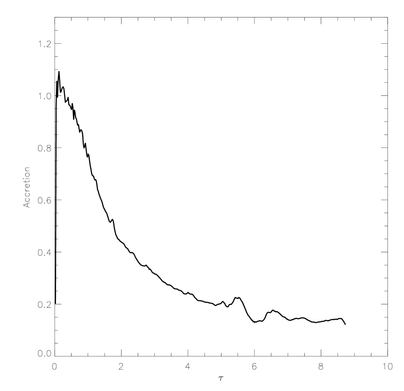
Figure 4: The dimensionless mass-accretion rate $\dot{m}\equiv G{\dot{M}}/a^{3}$ into the central cell as a function of dimensionless time $\tau\equiv at/r_{0}$. The spike at small times is an artifact of the starting conditions; $\dot{m}$ quickly drops to the value 0.975 expected from the unmagnetized SIS analysis (Shu 1977). Because of the non-isopedic magnetization of the present calculation, however, $\dot{m}$ continues to decline with $\tau$ as the infall encompasses ever more subcritical envelope. At $\tau=5.4$, when the central mass $m\equiv M/M_{0}$ is 56% of the expected final value of $\surd 2$, growing oscillations of the pseudodisk caused by numerical difficulties akin to those described in Allen et al. (2003a,b) lead to increasingly inaccurate representations of the regions closest to the central star (see Fig. 6).

At time $t=0$, we initiate the inside-out collapse by adding a small seed mass in the central cell of the calculation. The resulting (non-dimensional) mass-infall rate $\dot{m}\equiv G{\dot{M}}/a^{3}$ is shown in Figure 4 as a function of dimensionless time $\tau\equiv at/r_{0}$. The values of $\dot{m}$ at small $\tau$ are close to the unmagnetized SIS value of 0.975. For $\tau\raise 1.29167pt\hbox{$>$}\kern-7.5pt{\lower 2.79857pt\hbox{$\sim$}}1$, as the wave of expanding infall engulfs ever more subcritical envelope material, the infall rate declines steadily from 0.975. By $\tau=5.4$, the dimensionless mass $m_{*}\equiv M_{*}/M_{0}$ in the central cell has accumulated 56% of its final value of $\surd 2$ anticipated from the 2-D axisymmetric analysis of §3. At this time, when the flow is trying to establish a delicate balance between magnetic levitation by the split monopole and the gravitation of the point mass at the center, numerical diffusion associated with the artificial viscosity in the code introduced to mediate accretion shocks (and other truncation errors) sets off growing oscillations that resemble those which plagued the late-time simulations of Allen et al. (2003a,b). The manifestation of these oscillations in the instantaneous mass accretion rate for $\tau>5.4$ can be seen in Figure 4. An extrapolation of the time-averaged behavior of $\dot{m}$ suggests that the final accumulated mass $m_{*}$ would be consistent with the theoretical value of $\surd 2$. Indeed, much of the infall into the center originates at late times from material high off the midplane flowing down field lines that have been pulled into the central cell by the gravitational collapse, and the total amount of such material is finite.

Figure 5 depicts the flow in the meridional plane at $\tau=0.1,1.0,2.5,$ and $5.4$ before serious numerical oscillations commence. The solid curves of each snapshot show the configuration of magnetic field lines; arrows depict the local flow direction; and isodensity contours are given by heavy dashed curves, with the densest portions highlighted by shading. For each frame, a split monopole emerges from the central cell, which pushes out the field lines threading an inflowing pseudodisk before the split monopole fields straighten to attach to the imposed background fields. The fields threading the midplane of the configuration, in turn, progressively push on their neighbors radially farther out to give the magnetic tension forces that suspend the outer envelope against the part of the gravity of the central mass point and the pseudodisk that is not resisted by the gas-pressure gradient. The field strengths throughout the regions of interest (apart from those that go through the central zone) are everywhere equal to or below background values. Except for the vertical flare of the flattened pseudodisk into a toroid-like configuration at large $x\equiv\varpi/r_{0}$, the pictures in Figure 5 for late times are much as we would have anticipated on the basis of the axisymmetric 2-D final-state analysis of this paper.

Figure 6 lends additional weight to the correspondence between the 2-D and 3-D axisymmetric calculations. Plotted here against the dimensionless radius $x\equiv\varpi/r_{0}$ at the midplane of the calculation are the projected mass density $\Sigma$ and vertical magnetic field $B_{z}$ (the only nonzero component at $z=0$) at a time $\tau=8.5$, when the accumulated central mass is within 66% of its expected final value of $\surd 2$ times $M_{0}$. The units for $\Sigma$ and $B_{z}$ are $B_{0}/2\pi G^{1/2}$ and $B_{0}$, respectively, the same as used to make the graphs in Figure 3 for the final state in the 2-D axisymmetric calculations. Allowing for the distortion of the central regions because of the numerical oscillations, we see that the 3-D axisymmetric theory at late times holds no surprises that could not be anticipated by the 2-D axisymmetric analysis.

4 Discussion and Summary

4.1 A Powerful Conjecture

Equations (38)–(43) give the most salient features of the formal solution for the “initial” and “final” states of the posed collapse problem in axisymmetric 2-D if we insist on strict field freezing. It is interesting that the central masses that result from the dimensional formula,

$$M_{*}=\surd 2M_{0}=\pi^{2}\surd 2{a^{4}\over G^{3/2}B_{0}},$$ (64)

can be made to correspond to stellar masses only if we choose values of $a=(kT/\mu)^{1/2}$ and $B_{0}$ that correspond to interstellar values, yet the physical determination of the mass eigenvalue occurs close to the star, where the local temperature $T$ and $B_{z}$ in the realistic situation are likely to differ considerably from their interstellar counterparts. How sensitive, therefore, are our numerical conclusions to the exact details of the model adopted to do the actual calculations, in particular, to the assumptions of isothermality (same temperature in initial and final state) and field freezing (same $dM/d\Phi$) in initial and final states?

Apart from numerical factors of order unity, we believe that our conclusions are generic. The following is a “proof” that does not quite live up to the standards of rigorous mathematics, but is powerful by astronomical standards. If there is to be a final equilibrium involving a highly flattened, nonrotating, configuration of matter immediately outside the star, the final state of equilibrium still has to satisfy equation (23). For realistic temperatures in the pseudodisk (i.e., not approaching values comparable to that at the center of the star), the pressure gradient term in equation (23) is negligible in comparison the stellar gravity term $-M_{*}$ throughout the inner pseudodisk. Similarly, as long as the mass contained in the pseudodisk from the stellar surface out to radius $\varpi$ is less than the stellar mass $M_{*}$ multiplied by $\lambda(\varpi)$ times $\bar{\lambda}$ where $\bar{\lambda}$ is some appropriate average value in the pseudodisk, the contribution from the integral is negligible in comparison with the stellar gravity term. (This is always true for $\varpi$ near the inner edge $R_{*}^{+}$.) Thus, the only way to satisfy equation (23) is to have the split-monopole levitate the inner pseudodisk against the stellar gravity, i.e., the mass-to-flux ratio in the inner pseudodisk must have an inverse relationship to the stellar mass-to-flux ratio:

$$\lambda_{*}\lambda(R_{*}^{+})=1.$$ (65)

This elegant equation is the generalization of our eigenvalue determination for the final-state problem.

Suppose now that the initial cloud that gave rise to the collapsed final state has a flux-to-mass distribution given by

$${d\Phi\over dM}=2\pi G^{1/2}f^{\prime}\left({M\over M_{0}}\right),$$ (66)

where $M_{0}$ is no longer necessarily given by equation (7) but is equal, say, to the observed value where the cloud turns from being supercritical (core) to subcritical (envelope). We suppose therefore that the function $f^{\prime}(m)$ in equation (66) is a monotonically increasing function of its argument with the properties $f(0)=0$ and $f^{\prime}(1)=1$. Assuming strict field freezing in the transition from the initial to final state, and carrying out an integration of equation (66), we find that the flux to mass ratio of the final star is given by

$${\Phi_{*}\over M_{*}}=2\pi G^{1/2}f\left({M_{*}\over M_{0}}\right){M_{0}\over M_{*}}.$$ (67)

Denoting $m_{*}\equiv M_{*}/M_{0}$, and identifying $\lambda(R_{*}^{+})=[f^{\prime}(m_{*})]^{-1}$ and $\lambda_{*}=m_{*}/f(m_{*})$, equation (65) obtains the general solution for the multiple $m_{*}$ of $M_{0}$ that will fall into the star as the positive root of the equation:

$$f(m_{*})f^{\prime}(m_{*})-m_{*}=0.$$ (68)

For the special case, $f(m)=m^{2}/2$, we recover the eigenvalue solution $m_{*}=\surd 2$ of §2.

Equation (68) is a remarkable result. It claims the following. Start with a magnetized cloud of arbitrary shape and size (much bigger than a star) that has a dimensionless flux-to-mass distribution $f(m)$, where $m$ is the mass $M$ in units of the core mass $M_{0}$ (the supercritical part of the cloud) within magnetic flux $f$, which is $\Phi$ in units of $2\pi G^{1/2}M_{0}$. Then, without doing any calculations other than finding the root to equation (68), we are able to predict accurately the final mass of a star from the ideal MHD collapse of this cloud.

The initial conditions could contain an arbitrary amount of initial rotation, whose elimination by magnetic braking when field freezing holds – see Allen et al. (2003b) – will ensure the assumption of a single rotating star as the final state. The initial state also needs not be a configuration of equilibrium or near-equilibrium. It could contain sizable turbulent fluctuations in the density and velocity fields – particularly in the magnetically subcritical envelope – these will dissipate without having any effect on the final state. Sufficiently large turbulent fluctuations in the supercritical core (which are not seen in the cores that give rise to low-mass star formation) could give rise to temporary fragments, but in the presence of trapped stellar or pseudodisk flux which will stir the surrounding cloud envelope, the fragments are likely to lose all their orbital angular momentum and merge into a single final object. Finally, the thermal history can be arbitrarily complex. This will also have no effect on the final state, provided that radiation pressure on dust grains does not come into play (true for low-mass stars) and the temperature in the inner pseudodisk does not approach virial values.

4.2 Speculations

For realistic astronomical application, the weakest link in the above argument is, of course, the assumption of field freezing. Indeed, nearly fifty years ago, Mestel & Spitzer (1956) recognized that field freezing would predict stars at birth with surface magnetic fields of many megaguass, contrary to the observational evidence. They also pointed out (Mestel 1965, 1985; Spitzer 1968) that conservation of angular momentum in the gravitational collapse of stars from interstellar clouds would lead to absurd rotational velocities of the final objects, again contrary to the observational evidence. They proposed that a solution be found to link these two problems via magnetic braking and field slippage. We now propose to link the two classical problems of magnetic flux loss and angular momentum redistribution to the third great problem of star formation: What processes define the masses of forming stars? We even believe that the breakdown of field freezing plays a fundamental role in the fourth great problem of star formation: What determines whether gravitational collapse produces binary (or multiple) stars versus single stars surrounded by planetary systems? (See, e.g., the discussion of Galli et al. 2000 and the simulations of Nakamura & Li 2003.)

The formal answer given by equation (68) to what determines stellar masses is magnetic levitation. But levitation by a stellar split monopole leads to numerically unacceptable surface magnetic fields for the central star, as well as to the wrong prediction that magnetic fields should be weaker in the regions adjacent to newly formed stars than the surrounding molecular cloud (see Figs. 3 and 6 as well as Fish & Reid 2003). Is it possible that magnetic reconnection of the type contemplated by Galli & Shu (1993b, see also Mestel & Strittmatter 1967) completely eliminates the stellar monopole (except for some small seed fields needed to start stellar dynamo action)? After all, the strong sheet current corresponding to the reversal of field lines across the midplane of a split monopole will dissipate in the presence of finite resistivity. The dissipation of the sheet current corresponds to the annihilation of field lines just above and below the midplane. The magnetic pressure of remaining field lines presses toward the midplane to replace the lines that have been annihilated. They are annihilated in turn. The result is an ever weaker split monopole, which continues to lose strength by sheet current dissipation until the sheet current and the split monopole are both gone. (In practice, this dissipation would occur throughout the process of central mass and flux accumulation and not just in the final state.)

A vanishingly small split monopole, $\lambda_{*}\rightarrow\infty$ in equation (65), requires $\lambda(R_{*}^{+})\rightarrow 0$ if magnetic levitation is still to do its work. The only material so heavily magnetized outside the star (if magnetic flux were preserved even approximately in the rest of the system where the fields are not so severely pinched) comes from far out in the original model cloud. In other words, with no split monopole at the center to help it, magnetic suspension of the cloud envelope alone cannot withstand the very large gravity just above the surface of the star, and the infall would continue until the star has accumulated the entire molecular cloud (or stellar evolution intervenes).

But this possibility also contradicts the observational evidence. Therefore, imagine next that there is no electrical resistivity, but there is ambipolar diffusion. Unlike electrical resistivity, ambipolar diffusion cannot destroy magnetic flux, but it can redistribute it. Can ambipolar diffusion (or C shocks, see Li & McKee 1996) transfer the flux from material before it became incorporated into the star and redistribute it over a much wider area of a static pseudodisk, so that the resultant fields are not such an embarrassment relative to observations? On a larger scale the levitation provided by such fields could serve to prevent the infall of the cloud envelope. The difficulty of such a scheme is that there is only suspension to keep the static pseudodisk from falling into the star, and we proved in this paper that suspension without levitation cannot do such a job.

Keplerian rotation provides an excellent barrier to infall, so can the conversion of magnetized pseudodisk into a magnetized Keplerian disk provide the needed buttress to prevent the inward advance of the cloud envelope? The question is especially cogent now that Allen et al. (2003b) have demonstrated that centrifugally supported disks cannot arise in realistically magnetized models of rotating gravitational collapse unless the assumption of field freezing is abandoned in the pseudodisks and disks of star formation (see, also, Krasnopolsky & Königl 2002 for examples of formation of centrifugally supported disks in cases of low, prescribed, efficiency of magnetic braking in the presence of ambipolar diffusion). But strongly magnetized, rapidly rotating disks will develop magnetocentrifugally driven disk winds (Blandford & Payne 1982, Königl & Pudritz 2000), which will provide dynamic rather than static levitation. Thus, ultimately, the realistic solution to the problem of obtaining stellar masses from the gravitational collapse of large interstellar clouds will end up invoking wind-limited mass infall (Shu & Terebey 1984). Moreover, numerical simulations of Keplerian disks threaded by such a network of open field lines show them to quickly fall into the innermost regions of the disk (Gammie & Balbus 1994, Miller & Stone 1997), concentrating all the trapped flux into a narrow annulus that makes the subsequent outflow indistinguishable from an X-wind.

X-winds will also arise in the alternative extreme scenario of all electrical resistivity and no ambipolar diffusion, if Keplerian disks appear outside accreting protostars (Shu et al. 1988, 1994, 2000). In this case, although the stellar split monopole will eventually disappear because of field annihilation (eliminating the magnetic braking by long lever arms that prevents the formation of Keplerian disks in the simulations of Allen, Li, & Shu 2003), the operation of a stellar dynamo can replace such fields with those that have a dipole or higher multipole structure at the stellar surface (Mohanty & Shu 2003). The interaction of these dynamo-driven fields with the surrounding accretion disk, and the subsequent opening of the stellar field lines (or the simple pressing of the remnant interstellar field lines against the magnetopause) can then create an X-wind. The attractiveness of either proposal relative to that of static levitation is one of efficiency. Newly formed stars do not need 10 megaguass fields to halt the inflow of gravitational collapse. Surface fields of a few kilogauss, when combined with the rapid rotation from an adjoining accretion disk, suffice to provide dynamic levitation (a physical blowing away) of cloud envelopes.

In the real situation, electrical resistivity and ambipolar diffusion are probably equally important in the disks and pseudodisks around young stars. Since we have argued for X-winds as a likely outcome for the two extreme assumptions, we believe it is also the likely outcome in all intermediate cases.

4.3 From Isolated Star Formation to Distributed Star Formation

Imagine a large magnetized cloud which is overall subcritical, and therefore probably fairly flattened, but which contains many dense pockets (cloud cores) that are supercritical. (We are supposing that the discussion of §4.1 can be generalized to more than a single core.) Each of the cores can undergo inside-out collapse. If they later generate a magnetocentrifugally driven wind, they can each dynamically levitate their neighboring subcritical envelopes and prevent star formation from being anywhere near 100% efficient. A general inefficiency for forming stars is consistent with the observational evidence, except possibly for situations involving the bound-cluster mode of star formation. The supersonic turbulence and other complex factors in the subcritical common envelope play no dynamical role once the cores go into collapse and generate their winds, but the winds may play a crucial role in sustaining the observed turbulence and overall filamentary morphology of the cloud (Allen & Shu 2000). In turn, as discussed below, the turbulence in the general envelope may ultimately help set the mass distribution of molecular cloud cores before the onset of gravitational collapse, and therefore the initial-mass-function of forming stars.

How did the cloud get so many supercritical cores in a general environment that is subcritical? One answer proposed by Shu et al. (1987, see also Lizano & Shu 1989) is ambipolar diffusion acting as a background process in all molecular clouds. Their name for this process was “the isolated mode of star formation,” but in the present generalization, we refer to it as “the distributed mode of star formation.”

If ambipolar diffusion is the mechanism that condenses many cores from large cloud envelopes, it represents a kind of magnetic fragmentation. Whether this fragmentation occurs slowly or not relative to dynamical timescales may depend on the contractive and diffusive enhancements one ascribes to turbulence dissipation and fluctuations (Myers & Lazarian 1998, Myers 1999, Adams & Fatuzzo 2002, Zweibel 2002). In any case, the first supercritical core to appear from the gravitational contraction of any dense pocket of gas and dust has, by definition, a vanishingly small mass $M_{0}$, since the transition from subcritical to supercritical is made gradually. Unless dynamically compressed, such a core is not immediately unstable to inside-out gravitational collapse; it has to evolve by further ambipolar diffusion (and perhaps turbulent decay) to reach a state of sufficient central concentration. In the numerical simulations performed to date of this process, the exact state of runaway collapse depends on the outer boundary conditions that are imposed (see, e.g., Nakano 1979; Lizano & Shu 1989; Tomisaka, Ikeuchi, & Nakamura 1990; Basu & Mouschovias 1994; Li 1998). When those boundary conditions are applied at infinity, and the evolution is approximated as quasi-static, our group has argued for pivotal states that resemble singular isothermal toroids (Li & Shu 1996, Allen et al. 2003a), which are close relatives in their density distributions (but not flux distributions) to the magnetized SISs studied in this paper.

The details for cloud core structure are not important for the present application. Recently, Motte, André & Neri (1998), Testi & Sargent (1998), and Motte et al. (2001) have found that the mass distributions of cloud cores as mapped by dust emission in turbulent molecular clouds resemble the empirical initial mass function (IMF) of newly formed stars (Salpeter 1955, Scalo 1986). The weighting of cloud cores toward small (typically solarlike) masses instead of toward large masses (typically thousands of $M_{\odot}$) as in cloud clumps (sometimes called dense cores) is particularly striking. Lada & Lada (2003; see also Lefloch et al. 1998, and Sandell & Knee 2001) make the interesting suggestion that outflows may transform the mass-spectrum of cloud clumps, which resembles the mass distribution of embedded clusters, to the mass-spectrum of cloud cores, which resembles the mass distribution of stars. In what follows, we suggest a mechanistic process for performing such a task in a statistically invariant way, both in the distributed and the clustered modes of star formation, if outflows ultimately provide a major source of the turbulence present in star-forming clouds.

4.4 Initial Mass Function

As an example of how the processes described in this paper can determine the stellar IMF (see also Silk 1995 and Adams & Fatuzzo 1996), we consider the contribution lent by turbulent velocities $v$ to the support of molecular clouds. At a heuristic level, we imagine that $v$ can be added in quadrature to the isothermal sound speed $a$ in formulae that involve the gravitational constant $G$ (e.g., Stahler, Shu, & Taam 1980; Shu et al. 1987; McKee 2003; Pudritz 2003). For even greater simplicity, we use $v$ below to mean the turbulent velocity when the turbulence is supersonic, and we substitute $a$ for $v$ when that turbulence is subsonic.

From IRAM and CSO observations of molecular clouds, Falgarone & Phillips (1996) find that CO line-profiles have high-velocity wings indicative of supersonic turbulence. This interpretation is supported by the study of Falgarone (2002) who argues that the structure of molecular clouds is characterized by a unique power-law in mass, except possibly for a lower scale defined by cloud cores (Blitz & Williams 1999). We adopt such a description and assume that the mass of magnetized molecular-cloud material with turbulent velocity between $v$ and $v+dv$ in 1-D is given by the power-law distribution,

$${\cal M}(v)\,dv\propto v^{-s}\,dv,$$ (69)

where $s$ is a positive number. To avoid divergence of the integrated mass at very small $v$, we cut off the distribution (69) when $v$ becomes smaller than the thermal line-width $a$, noting that the important applications occur at $v\raise 1.29167pt\hbox{$<$}\kern-7.5pt{\lower 2.79857pt\hbox{$\sim$}}1$ km s^-1.

To ensure that there is no confusion over what we mean by ${\cal M}(v)\,dv$, we emphasize that we have in mind a statistical sampling of a whole giant molecular cloud (GMC), or even of an ensemble of GMCs in an entire galaxy. As a practical way to measure ${\cal M}(v)\,dv$, at least at relatively large $v$’s (a few km s^-1), imagine getting the integrated spectrum of a GMC in the line wings of some optically thin species, after we remove the effects of a systematic velocity field, and determining the mass with random velocity between $v$ and $v+dv$ along the line of sight. Then our derivation below holds assuming that the same functional form ${\cal M}(v)$ extrapolates to $v\raise 1.29167pt\hbox{$<$}\kern-7.5pt{\lower 2.79857pt\hbox{$\sim$}}1$ km s^-1 and to the material in molecular cloud cores.

With this understanding, we further suppose that the core mass $M_{0}$ can be approximated as (see eq. [7]):

$$M_{0}=m_{0}{v^{4}\over G^{3/2}B_{0}},$$ (70)

where the coefficient $m_{0}$ has a probabilistic distribution centered about $\pi^{2}$ with a variance of a factor of a few (see §4.6). Values of $m_{0}$ smaller than the typical $\pi^{2}$ arise because turbulence, if compressive rather than expansive, can act to decrease as well as to increase the stability of some fiducial statistical equilibrium. Suppose now that the final stellar mass is some fixed fraction of $M_{0}$ (say, 1/3; see §4.6):

$$M_{*}\sim{1\over 3}M_{0}\sim{m_{0}v^{4}\over 3G^{3/2}B_{0}}.$$ (71)

With a stellar mass-accumulation rate behaving as (2/3 times the infall rate) $\dot{M}_{*}\sim 2v^{3}/3G$ (cf. Shu et al. 1987), we get a characteristic formation time,

$$t_{\rm sf}\equiv{M_{*}\over\dot{M}_{*}}\sim{m_{0}v\over 2G^{1/2}B_{0}}={m_{0}^{1/2}r_{0}\over 2v},$$ (72)

where we have adopted equation (8) with $a$ and $\pi$ replaced, respectively by $v$ and $\surd m_{0}$ to estimate the core radius $r_{0}$. The infall rate could exceed $v^{3}/G$ by a factor of a few if static magnetic fields contribute to core support before collapse, and if pivotal states contain nonzero contraction velocities (Allen et al. 2003a, b). The characteristic time $t_{\rm sf}$ would then typically measure $\sim 10^{5}$ yr, rather than a few times this value.

We further suppose that $B_{0}$ scales with $v$ as

$$B_{0}\propto v^{p},$$ (73)

where $p$ is again a positive number. The mass of stars formed during any fixed interval of time $t_{\rm sf}$ with stellar masses between $M_{*}$ and $M_{*}+dM_{*}$ is now given by

$$M_{*}{\cal N}(M_{*})\,dM_{*}=\varepsilon{\cal M}(v)\,dv\propto M_{*}^{-(s+3-p)/(4-p)}\,dM_{*}.$$ (74)

In equation (74), $\varepsilon$ is an overall efficiency of turning molecular clouds into stars and is given by

$$\varepsilon={F\over 3},$$ (75)

where $F$ is the cumulative fraction of molecular cloud mass in the region that has existed as star-forming cores. Of the currently observable cores, a fraction $t_{\rm sf}/(t_{\rm sf}+t_{\rm AD})$ exists as cores with actively accreting embedded protostars, and a complementary fraction $t_{\rm AD}/(t_{\rm sf}+t_{\rm AD})$ exists as starless cores. In the latter expressions, $t_{\rm AD}$ is the time required for ambipolar diffusion and the decay of turbulence to transform a core with a critical level of magnetization to one in a pivotal state at the onset of protostar formation.

Except for the normalization factor $\varepsilon$, where we have adopted the observer’s definition of star formation efficiency as the mass of formed stars divided by the mass of total starting material in the region, equation (74) corresponds to Salpeter’s (1955) IMF for low- and intermediate-mass stars if

$${s+3-p\over 4-p}=4/3,\qquad i.e.,\;{\rm if}\qquad s={7-p\over 3}.$$ (76)

In the above, we have taken the liberty of approximating Salpeter’s 1.35 by $4/3$. One attractive combination satisfying the 4/3 rule is $p=1$ and $s=2$. This case corresponds to equal $t_{\rm sf}$ for stars of all masses (eq. [72]) and Lorentzian line wings (eq. [69]).

From observation (Masson & Chernin 1992) and theory (Li & Shu 1996), it is known that bipolar outflows produce swept-up mass distributions that satisfy equation (69), with $s$ close to, but perhaps slightly smaller than 2, except at the highest velocities, where $s$ can be significantly larger than 2 (Lada & Fich 1996). It is not known, however, whether the same distribution applies after the gas has decelerated from velocities of order 10 km s^-1 to those of order 1 km s^-1. The assumption that $B_{0}$ scales linearly with $v$ ($p=1$) agrees with the estimate by Myers & Fuller (1993) that stars of all masses take $\sim$ (a few times) $10^{5}$ yr to form once gravitational collapse starts. A positive correlation will exist between $B_{0}$ and $v$ if regions with larger turbulent velocities require supercritical cores to reach higher mean densities before they become self-gravitating, resulting in a greater compression of the mean magnetic field threading the core. The Salpeter slope in equation (74) does not depend sensitively on the exact choice for $p$ if $s=2$.

In this paper, to match the properties of Taurus cores, we have adopted a normalization of $B_{0}=30\;\mu$G when $v=a=0.2$ km s^-1. With this normalization, the minimum stellar mass to result from equation (71) is nominally 0.5 $M_{\odot}$ if we take $m_{0}$ to have a typical value of $\pi^{2}$. In actual practice, 0.5 $M_{\odot}$ is close to the flattening of the observed Galactic IMF for $M_{*}{\cal N}(M_{*})$ (Scalo 1986), but significant numbers of stars form in the Orion Trapezium region down to and below the hydrogen-burning limit $0.08$ $M_{\odot}$ (cf. Fig 10 of Lada & Lada 2003). In the current physical picture, stars can form with masses smaller than 0.5 $M_{\odot}$, because there is a distribution in the value of $m_{0}a^{4}/B_{0}$ for different regions. In this context, it may be meaningful that Taurus appears to be deficient in brown dwarfs in comparison with the Orion Trapezium (Luhman 2000), consistent with our earlier suggestion that the effective value of $B_{0}$ may be statistically lower in the former region. But it could be that a significant number of brown dwarfs are initially formed as companions to normal stars and that there are larger numbers of “free-floating” brown dwarfs in Orion than in Taurus because of the greater role of binary disruption in the cluster environment (Kroupa 1995). It could also be that a limited form of Hoyle’s (1955) fragmentation picture can still apply to turbulent, magnetized, cores if the eventual decoupling of magnetic fields occur sufficiently rapidly in realistic non-ideal MHD (Galli et al. 2000, Nakamura & Li 2003).

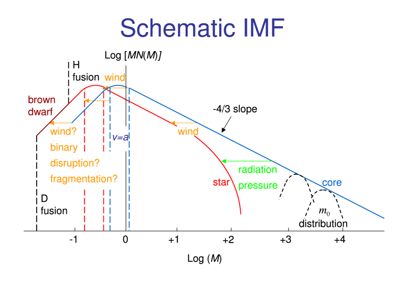
Figure 7: The distribution $M{\cal N}(M)$ plotted schematically for cloud cores and young stars against mass $M$ in a log-log format. The unit of mass is solar masses, and the vertical scale is arbitrary. Cloud cores of given $v^{4}/G^{3/2}B_{0}$ have a statistical distribution of masses as indicated by the two bell-functions at large core masses, because of the variation of the coefficient $m_{0}$. The convolution of a bell distribution with a $-4/3$ power-law distribution of $v^{4}/G^{3/2}B_{0}$ produces the solid curve labeled by “core.” This distribution reaches a natural peak when $v$ equals the thermal sound speed $a$, which itself has a range of values indicated schematically by the two vertical dashed lines. A further extension toward “subthermal values” (beyond that expected from the distribution of $m_{0}$) may result if fragmentation of thermal cores can occur during the subsequent collapse, or if binary disruption occurs to unbind substellar companions from normal stars. Without fragmentation or binary disruption, the core mass is reduced to the star mass by the arrows depicting the effects of YSO winds and radiation pressure acting on dust grains during the gravitational collapse of any core. The hydrogen- and deuterium-burning limits that separate stars from brown dwarfs and brown dwarfs from (free-floating) planets are indicated. No discontinuity at the H-burning limit occurs, because pre-main-sequence stars are observed to lie in the Hertzsprung-Russell diagram above the line (Zero-age-main sequence) where they would start burning hydrogen; thus hydrogen-burning could not have played a role in the determination of their initial masses. On the other hand, T Tauri stars do exhibit a “birthline” (Stahler 1983), which has been associated with deuterium burning, and deuterium burning could play a role in the shape of the lower-mass end of the stellar IMF (Shu & Terebey 1984).

Apart from the different behaviors at low stellar masses, departures from a $-4/3$ power law in the observed IMF appear also at the highest stellar masses. We believe that an exponent for $M_{*}{\cal N}(M_{*})$ steeper than $-4/3$ can arise at large stellar masses because radiation pressure acting on dust grains aids YSO winds to reduce $M_{*}$ as a fraction of the initial core mass $M_{0}$ (Wolfire & Cassinelli 1987, Jijina & Adams 1996). If this interpretation is correct, the non-power-law features in the stellar IMF contain clues on how stars help to limit their own masses by blowing away cloud material that might have otherwise fallen gravitationally into the stars (cf. Adams & Fatuzzo 1996). Figure 7 depicts pictorially the ideas of this subsection.

4.5 Embedded Cluster Formation

Our derivation of the IMF formally seems to hold only for the distributed mode of starbirth, where competitive accretion does not occur. But apart from the deficit of brown dwarfs, the IMF of YSOs does not appear to be different in Taurus compared to clusters or the general field (Kenyon & Hartmann 1995). Moreover, the sometimes evoked picture of protostars growing by Bondi-Hoyle accretion as they move freely in a background of more-or-less smooth clump gas may be flawed. After all, stars do not appear half formed from nowhere; they probably have to grow by gravitational collapse and infall of small dense cores that are themselves self-gravitating substructures in the cloud clump. The gravitational potential associated with the cores forms local minima that are sharper, although perhaps less deep in absolute terms, than the large bowl that represents the smoothed gravitational potential of the clump and associated embedded cluster. The tidal forces of the latter will not rip asunder the small cores if their mean densities are appreciably larger than the mean density of the background clump/cluster gas (which is the so-called Roche criterion).

In this regard, it is informative to note that the mean density inside a sphere of radius $r_{0}$ of a uniformly magnetized SIS is given by

$$\bar{\rho}_{\rm core}={2a^{2}r_{0}/G\over 4\pi r_{0}^{3}/3}={3B_{0}^{2}\over 2\pi^{3}a^{2}}.$$ (77)

For $a=0.2$ km s^-1 and $B_{0}=30\;\mu$G, $\bar{\rho}_{\rm core}$ has a numerical value $1.1\times 10^{-19}$ g cm^-3 $\approx$ $1.6\times 10^{3}$ $M_{\odot}$ pc^-3. This core density is larger than the average density of any observed clump forming an embedded cluster in the local GMCs of our Galaxy, except perhaps for the central regions of the very densest clumps (Lada & Lada 2003, Table 1). In the central regions of the densest clumps, individual small cores may merge, yielding the large cores that give rise to massive stars. (We presume that such merger processes and large cores are part of the “turbulent” spectrum in eq. [69].) However, the actual part of the core that forms a star is on average 9 times denser yet than the value ${\bar{\rho}}_{\rm core}$, so forming low-mass stars can survive the neighboring appearance of luminous high-mass stars, although the remnant envelopes, pseudodisks, and disks not truncated by the tides of the central cluster/clump, may be photoevaporated away by the ultraviolet radiation field of the H II regions in which they are embedded (Johnstone, Hollenbach, & Bally 1998). In contrast, the low-mass stars being born at the centers of the small cores at the peripheries of the clump, are in no greater danger of wandering away from those centers than we risk falling off the Earth because it orbits the Sun with a far deeper gravitational potential.

We do need to worry about the disruption of the cores from hydrodynamic effects as they orbit inside the clump/cluster. However, such orbital effects are probably mitigated by the magnetization of the clump and cores. This magnetization dilutes the effect of gravitation (if both clump and core are supercritical); and the net forces can actually turn repulsive if the clump (common envelope of the cores) is subcritical. Thus, the orbital motions of cores are likely to be sub-virial with orbital times to cross the clump in excess of the time $t_{\rm sf}$ required to form individual stars. The individual cores may hold together better as entities than envisaged in the standard picture of a highly turbulent and chaotic clump.

As long as the growing protostar (which feels only gravitational forces if it completely destroys its accreted interstellar flux by magnetic reconnection) is trapped by the local potential minimum of its parent core, the situation will resemble, to zeroth order, the case of isolated star formation. Sooner or later, such a protostar will develop an X-wind and begin to blow away its placental core. The fact that the common envelope in a cluster environment may be mildly supercritical, instead of subcritical, may not make too big a difference on our (admittedly crude) estimate that only 1/3 of the initial supercritical core will end up falling onto the star (see below). Indeed, in the present context, the 1/3 figure takes on added significance. As an extreme, we may think of a turbulent clump which is supercritical everywhere as completely packed with cores, with no surrounding “common envelope” (packed like “kernels” [of corn on the cob] in the nomenclature of P. C. Myers). In that case, the efficiency of wind-limited star formation for the clump is the same as the average efficiency for a typical core, which we have taken to be 1/3 (see eq. [71]). The same result, $\varepsilon=1/3$, can be obtained from equation ( 75) by setting $F=1$. It is then interesting to note that the maximum star-formation efficiency $\varepsilon$ deduced by Lada & Lada (2003, Table 2) for embedded star clusters is indeed 33%.

To zeroth order, therefore, the clustered mode of star formation under present-day levels of magnetization may be considered as an extreme form of the distributed mode of star formation, which is itself a generalization of the isolated mode of star formation. Otherwise, it becomes a total coincidence that the IMFs found in many different environs of star formation, crowded or dispersed, are similar, with departures, if any, only at the lower end of the mass spectrum (Lada & Lada 2003).

4.6 Conclusion

For the mass scale $M_{0}$ of cloud cores to play its part in setting stellar masses, cloud envelopes need to be not highly supercritical. Indeed, for highly supercritical (e.g., unmagnetized) and turbulent clouds it is difficult even to define exactly what one means by a “core” or “clump” except by Roche-lobe or “sphere of influence” arguments. Moreover, without outflows to halt infall, artificial numerical means to pump in local turbulence (Klessen 2000) in combination, perhaps, with the “Jeans swindle” (Gammie 2003) is needed to keep the star-formation efficiency of supercritical regions that are overall gravitationally bound from approaching unity, contrary to the observational evidence. To understand the overall low efficiency of star formation, it would be best if the bulk of molecular clouds, except for their cores, were subcritical or only marginally critical. Unfortunately, observers have found no regions of molecular clouds that are definitely subcritical (Crutcher & Troland 2000). This may be because they are biased to looking at regions where star formation has already taken place, and such regions are necessarily supercritical. Allowing for various projection corrections, Shu et al. (1999) argued that most Zeeman measurements to date are consistent with the presence of a near-critical level of magnetization in molecular clouds. This leaves us optimistic about the fundamental correctness of the basic program begun by Mestel and Spitzer (1956) nearly fifty years ago.

Simple numerical estimates suffice to make our case here. On average, the envelopes of GMCs possess 4 magnitudes of visual extinction (e.g., Blitz & Williams 1999). With the usual caliberation that a number-column density of hydrogen $N_{\rm H}=1.9\times 10^{21}$ cm^-2 yields 1 mag of visual extinction and that a helium atom accompanies each 10 hydrogen atoms, the observed extinction through envelopes corresponds to a mass-column density equal to

$$N_{\rm H}(1.4)m_{\rm H}=0.018{\rm g}\;{\rm cm}^{-2}.$$ (78)

Zeeman measurements yield the component of the magnetic field along a typical line of sight through a GMC as $B_{\rm los}$ = 10 $\mu$G (Crutcher & Troland 1999). This combination gives an apparent dimensionless ratio of magnetic field to mass-column density along the line of sight equal to

$${B_{\rm los}\over 2\pi G^{1/2}N_{\rm H}(1.4m_{\rm H})}=0.34$$ (79)

in the envelopes of GMCs. For a flat sheet of surface density $\Sigma$ threaded perpendicularly by a magnetic field $B_{z}$, viewed at an angle $\theta$ with respect to the normal to the sheet, $B_{\rm los}=B_{z}\cos\theta$ systematically underestimates the true field strength $B_{z}$, and $1.4m_{\rm H}N_{\rm H}=\Sigma/\cos\theta$ sytematically overestimates the true surface density $\Sigma$. Since $\cos^{2}\theta$ averaged over a hemisphere equals 1/3, we see that equation (79) is close to the expectation value for a sheet which is exactly critically magnetized:

$${B_{z}\over 2\pi G^{1/2}\Sigma}=1.$$ (80)

Without bothering to argue about whether better numerical values or better corrections might make the right-hand side of equation (80) greater or less than unity, we will merely reiterate Shu et al.’s (1999) observation that it is probably no coincidence that modern-day GMCs have near-critical levels of magnetization. Highly subcritical clouds are too non-self-gravitating to become molecular clouds; they are present in galaxies as H I clouds (Heiles 2003). On the other hand, highly supercritical clouds are too vulnerable to gravitational collapse; they have long since disappeared to become the interiors of stars. McKee’s important point that the ultraviolet photons associated with the interstellar radiation field suffice to keep regions with less than 4 mag of visual extinction too highly ionized to permit appreciable ambipolar diffusion then leads naturally to the idea of magnetically regulated star-formation (McKee 1989).

As a consequence, ambipolar diffusion can act to produce distinctly supercritical regions only in the cores of molecular clouds. Many simulations (e.g., Lizano & Shu 1989, Basu & Mouschovias 1994) show that such cores of mass $M_{0}$, equatorial radius $r_{0}$, and mean magnetic field $\bar{B}$ become susceptible to gravitational collapse once the dimensionless mass-to-flux ratio acquires a value of about 2:

$$\bar{\lambda}\equiv{2\pi G^{1/2}M_{0}\over\pi r_{0}^{2}\bar{B}}\approx 2.$$ (81)

The dilution of gravity $(1-\bar{\lambda}^{-2})=3/4$ (Shu & Li 1997) associated with this mean level of magnetization is not severe, and if the same core is supported against gravity largely by turbulent velocity $v$ (as measured in any single dimension), then virial equilibrium requires

$$2\cdot{3\over 2}M_{0}v^{2}\approx{GM_{0}^{2}\over r_{0}}.$$ (82)

Solution of equations (81) and (82) yields

$$M_{0}\approx{9v^{4}\over G^{3/2}\bar{B}},\qquad r_{0}\approx{3v^{2}\over G^{1/2}\bar{B}}.$$ (83)

When we identify $\bar{B}$ with $B_{0}$, equation (83) for $M_{0}$ and $r_{0}$ differ from our expressions (7) and (8) for the same quantities only in the replacement of $\pi$ by 3.

If turbulent cores are barely bound rather than fully virialized – as implied by some suggestions that star-forming cores are produced as dynamical objects rather than as ”equilibrium” states – then the factor of 2 should be removed from the left-hand side of equation (82). In fact, since fluctuations can exist on either side of virial equilibrium, we estimate that $M_{0}$ given by an expression for star-forming, bound cores such as equation (70) can have a coefficient $m_{0}$ that might vary by a factor as much as 4 about a central value of 3 or $\pi$. This crude estimate is depicted schematically in Figure 7 showing the typical distribution of $m_{0}$.

The following reasoning underlies the central idea behind our rough estimate that the final mass for the formed star is typically one-third of the core mass, $M_{*}=M_{0}/3$. As long as the infall encompasses only supercritical regions, the inflow of matter through the envelope and pseudodisk may be too strong for an incipient X-wind to reverse the infall completely (see Fig. 4). However, when the outwardly expanding wave of infall begins to encompass the subcritical envelope (which happens at a dimensionless time $\tau=1$ in Fig. 5) and the mass infall rate declines significantly below its standard value $\sim(1+H_{0})a^{3}/G$, with $H_{0}$ a measure of the static magnetic contribution to cloud-core support (Li & Shu 1996; Allen et al. 2003a,b), the X-wind may begin to blast its way to ever wider opening angles and push on the cloud magnetic fields that thread through the infalling pseudodisk to reduce the accretion rate further. The interaction may be quite complex, as the wind outflow rate itself may be a fraction ($\sim$ 1/3) of the mass inflow rate (Shu et al. 1988, 1994, 2000). Nevertheless, once outward motions are imparted to a significant portion of the surrounding cloud envelope, inertia and the “action at a distance” that is part of the effect of magnetic tension, may succeed in blowing away the infalling pseudodisk, even when the instantaneous wind rate from the central star drops to negligible values. Although detailed calculations are needed to quantify the estimates, which we are in the process of performing, comparison with the shape of the base of the outflow cavities in Class I sources suggests that the configuration at $\tau=2.5$ in Figure 5 may be amenable to complete reversal of the inflow. As an approximate guess, therefore, we suppose that 1/2 of the core mass $M_{0}$ will have dropped into the central regions before an X-wind can effectively halt the infall. Of this 1/2, only 2/3 has ended up on the star (1/3 has come out as an X-wind); thus, $M_{*}=(2/3)(1/2)M_{0}=M_{0}/3$. The entire description would then lend physical content to the observational definition that the transition from Class 0 to Class I marks the end of the phase of major infall in protostellar evolution (André, Ward-Thompson, & Barsony 1993).

In summary, the answer to the question posed by the title of our paper is a qualified “yes” – yes, magnetic levitation and suspension may help to define the masses of forming stars – but only in a dynamical context that involves rapid rotation and protostellar outflows. Knowing the relationship between stellar mass to core mass for any single region then reduces the problem of the stellar IMF to an explanation for the mass distribution of the cores of molecular clouds.

Appendix A: Comments on the Calculation of $K_{0}(\eta)$

The (force) integral-function $K_{0}(\eta)$ is related to a simpler (potential) integral-function:

$$H(\xi)\equiv{1\over 2\pi}\oint{d\varphi\over\sqrt{1+\xi^{2}-2\xi\cos\varphi}}.$$ (84)

It is trivial to show that $-\xi^{2}H^{\prime}(\xi)$ is equal to $K_{0}(\eta)$ if we set $\xi=1/\eta$. On the other hand, by making use of the even properties of the integrand and transforming $\psi\equiv\varphi/2$, we may write $H(\xi)$ itself in terms of the first elliptic integral $(\pi/2)E(\kappa)$:

$$H(\xi)={1\over 1+\xi}E(\kappa),$$ (85)

where

$$E(\kappa)\equiv{2\over\pi}\int_{0}^{\pi/2}{d\psi\over\sqrt{1-\kappa\cos^{2}\psi}},\qquad\kappa\equiv{4\xi\over(1+\xi)^{2}}.$$ (86)

Unlike the semi-infinite ranges of $\xi$ or $\eta$, $\kappa$ is bounded to lie within 0 and 1. This makes $E(\kappa)$ easy to tabulate and/or to approximate by empirical fitting formulae with high numerical accuracy (See Chapter 17 of Abramowitz and Stegun 1972). Note that $E(\kappa)$ has a logarithmic singularity at $\kappa=1$, i.e., the potential associated with a unit ring of matter at dimensionless radius $r$ is weakly singular at the position of the ring $\varpi=r$. The associated radial acceleration $K_{0}$ is large, but changes sign, as one crosses the ring.

Appendix B: Asymptotics of Flat Final State

We wish to solve the governing equation (48) for $x\gg 1$ where $\epsilon\ll 1$. For large $x$, the two most dangerous terms are $x$ times 1 and $-\surd 2$ that appear on the right-hand side of equation (48). We expect $\epsilon(x)$ to be very small at large $x$, in such a way that the left-hand side of equation (48) cannot be expected to balance either of these terms [otherwise, $\epsilon(x)$ would behave either as $-\ln x$ or as $-1/(x\surd 2)$ at large $x$, both of which violate the expectation that $\epsilon$ is everywhere positive when matter moves inward in gravitational collapse]. The only way that the two troublesome terms can be eliminated is if

$${\cal J}(x)\rightarrow-1\qquad{\rm and}\qquad{\cal I}(x)\rightarrow-\surd 2\qquad{\rm as}\qquad x\rightarrow\infty.$$ (87)

These properties are indeed fulfilled by the numerical solution.

The mathematical reason that the two constraints (87) are fulfilled individually, rather than in sum, is simple. Consider a value of $x$ so large that all of the contributions to the integrals defining ${\cal I}(x)$ and ${\cal J}(x)$ come from values of $y\ll x$ [because $\epsilon(y)$ becomes negligible for $y$ comparable to or much larger than $x$]. For $y\ll x$, $K_{0}(y/x)$ is well approximated by unity, and equation (49) and (50) become

$${\cal I}(\infty)=\int_{0^{+}}^{\infty}\epsilon^{\prime}(y)\,dy=-\epsilon(0^{+})=-\surd 2,$$ (88)

$${\cal J}(\infty)=\int_{0^{+}}^{\infty}{d\over dy}\left[y\epsilon(y)+{1\over 2}\epsilon^{2}(y)\right]\,dy=-{1\over 2}\epsilon^{2}(0^{+})=-1.$$ (89)

Thus, both constraints of equation (87) are automatically fulfilled if our solution satisfies the inner BC, $\epsilon(0^{+})=\surd 2$, and $\epsilon(y)$ goes to zero at large $y$ faster than $y^{-1}$. Since we anticipate that $\epsilon(y)$ is an analytic function of $y$ at infinity, we suppose it to have a Laurent series expansion,

$$\epsilon(y)={A_{2}\over y^{2}}+{A_{3}\over y^{3}}+\dots.$$ (90)

By numerical solution of the integro-differential equation (48), we determine the coefficient $A_{2}$ to be close to 1.

Figure 1: The normalized gravity kernel $K_{0}(\eta)$ and its associated “potential” function $H(\xi)$ defined in Appendix A, with $\xi=1/\eta$. Notice that both functions approach 1 at the origin and zero at the infinity.

Figure 2: Properties of the flat, final state. Shown in panels are (a) linear-linear plot of the numerically-determined eigenfunction $\epsilon(x)$, which denotes the difference in the mass enclosed within a given radius $x$ between the final and initial state; (b) log-log plot of $\epsilon(x)$, showing the power-law decay of the eigenfunction at large radii (the coefficient of the power-law plotted in dashed line is $A_{2}=1.1$); (c) distribution of the enclosed mass $m(x)$ in the final state (solid line) compared with that in the initial state (dashed line); and (d) the combination $1+{\cal J}(x)$, which is proportional to the total magnetic force due to levitation and suspension.

Figure 3: Distributions of the (dimensionless) column density and the strength of the vertical magnetic field on the flat pseudodisk in the final state (solid lines). Notice the reduction in both the column density and field strength at small radii compared with the initial distributions (dashed lines).

Figure 5: The infall flow direction (unit arrows) and magnetic field lines (solid curves) in the meridional plane at a dimensionless times $\tau=0.1,1.0.2.5,5.4$. Distances (axes), isodensity contours (heavy dashed curves), and isovelociy contours (light dotted curves) are plotted with $r_{0}$, $M_{0}/r_{0}^{3}$, and $a$ as the units of time, density, and speed. We have not plotted iso-field-strength contours because, except for the protostar, the entire region has magnetic field strength between the $0.3\,B_{0}$ and $B_{0}$ values that might have been used for contouring. At $\tau=0.1$, the flow is only slightly perturbed from what we may expect for the collapse of the unmagnetized SIS. At $\tau=1$, an infalling pseudodisk is apparent at small radii along the midplane. At large distances from the origin, a motion occurs primarily toward the magnetic axis, which carries field lines almost cylindrically to replace those that have been pinched inward by the point source at the center. At $\tau=2.5$, the inward bunching of field lines has grown sufficiently to prevent much further cylindrical concentration of field lines, and the gas flow becomes more nearly along field lines. As a consequence, a near-vacuum region forms close to the magnetic axis as most of the material above the midplane drains onto the pseudodisk. At $\tau=5.4$, the pseudodisk is very flat in the central regions, $x\equiv\varpi/r_{0}\raise 1.29167pt\hbox{$<$}\kern-7.5pt{\lower 2.79857pt\hbox{$\sim$}}0.5$, but it flares into an expected toroid-like structure farther out where the gravity of the central mass point no longer dominates the self-gravity and pressure forces of the envelope. Within the pseudodisk, there is still some radial flow into the central mass point (see Fig. [4]), which is still only 56% of the value $\surd 2$ times $M_{0}$ expected from the axisymmetric 2-D eigenvalue analysis.

Figure 6: Distributions of the (dimensionless) column density and the strength of the vertical magnetic field at the midplane for the 3-D time-dependent (axisymmetric) calculations at a dimensionless time $\tau=8.5$ (solid lines) in the same run as Figures 4 and 5. Notice the reduction in both the column density and field strength at small radii compared with the initial distributions (dashed lines). Close to the protostar, numerical difficulties are being encountered with field freezing because the curves for (normalized) $B_{z}$ and $\Sigma$ should not cross for the subcritical material outside of the stellar core. Apart from the numerical diffusion associated with the mediation of accretion shocks, this figure compares well with the 2-D (axisymmetric) final-state results of Figure 3.

References

- (1) Abramowitz, M. & Stegun, I. 1972, A Handbook of Mathematical Functions (New York: Dover)
- (2) Adams, F. C., & Fatuzzo, M. 1996, ApJ, 464, 256
- (3) Allen, A., & Shu, F. H. 2000, ApJ, 536, 368
- (4) Allen, A., Shu, F. H. & Li, Z.-Y. 2003a ApJ, submitted
- (5) Allen, A., Li, Z.-Y. & Shu, F. H. 2003b ApJ, submitted
- (6) André, P., Ward-Thompson, D., & Barsony, M. 1993, ApJ, 406, 122
- (7) Bachiller, R. 1996, ARAA, 34, 111
- (8) Basri, G., Marcy, G. W., & Valenti, J. A. 1992, ApJ, 390, 622
- (9) Basu, S. & Mouschovias, T. 1994, ApJ, 432, 720
- (10) Blandford, R. D. & Payne, D. G. 1982, MNRAS, 199, 883
- (11) Blitz, L., & Williams, J. P. 1999, in The Origin of Stars and Planetary Systems, ed. C. J. Lada & N. D. Kylafis (Kluwer), 3
- (12) Bodenheimer, P. 1978, ApJ, 224, 488
- (13) Bodenheimer, P., Burkert, A., Klein, R. I., & Boss, A. P. 2000, in Protostars and Planets IV, ed. V. Mannings, A. P. Boss, & S. S. Russell (Tucson: University of Arizona Press), p. 675
- (14) Bonnor, W. B. 1956, MNRAS, 116, 351
- Crutcher & Troland (2000) Crutcher, R. M. & Troland, T. H. 2000, ApJ, 537, L139
- (16) Ebert, R. 1955, Zeitschrift fur Astrophysics, 37, 217
- (17) Elmegreen, B. G. 2000, ApJ, 530, 227
- (18) Elmegreen, B. G. 2002, ApJ, 564, 773
- (19) Elmegreen, B. G. & Efrmov, Yu N. 1997, ApJ, 480, 235
- (20) Evans, N. J. 1999, ARAA, 37, 311
- (21) Falgarone, E. 2002, in Infrared and Submillimeter Space Astronomy, ed. M. Giard, J. P. Bernanrd, A. Klotz, & I Ristorcelli (EDP Sciences), 87
- (22) Falgarone, E., & Phillips, T. 1996, ApJ, 472, 191
- (23) Fatuzzo, M., & Adams, F. C. 2002, ApJ, 570, 210
- (24) Fish, V. L. & Reid, M. J. 2003, ApJ, submitted
- (25) Galli, D., Lizano, S., Li, Z. Y., Adams, F. C., & Shu, F. H. 1999, ApJ, 521, 630
- (26) Galli, D., & Shu, F. H. 1993a, ApJ, 417, 220
- (27) Galli, D., & Shu, F. H. 1993b, ApJ, 417, 243
- (28) Gammie, C. F., & Balbus, S. A. 1994, MNRAS, 270, 138
- (29) Gammie, C. F., Lin, Y. T., Stone, J. M., & Ostriker, E. C. 2003, ApJ, 592, 203
- (30) Glassgold, A. E., Najita, J., & Igea, J. 1997, ApJ, 480, 344
- (31) Hartmann, L. 2003, ApJ, 585, 398
- (32) Heitsch, F., MacLow, M., & Klessen, R. S. 2001, ApJ, 547, 280
- (33) Heiles, C. 2003, in preparation
- (34) Hoyle, F. 1953, ApJ, 118, 513
- (35) Hunter, C. 1967, in Relativity Theory and Astrophysics. Vol.2. ed. J. Ehlers (Providence, Rhode Island: American Mathematical Society), p. 169
- (36) Jijina, J, & Adams, F. C. 1996, ApJ, 462, 874
- (37) Jijina, J., Myers, P.C., & Adams, F. C. 1999, ApJS, 125, 161
- (38) Johns-Krull, C. M., Valenti, J. A., & Koresko, C. 1999, ApJ, 516, 900
- (39) Johnstone, D., Hollenbach, D., & Bally, J. 1998, ApJ, 499, 758
- (40) Kenyon, S. J., & Hartmann, L. 1995, ApJS, 101, 117
- (41) Klein, R. I., Fisher, R. T., Krumholz, M. R., McKee, C. F. 2003, Rev. Mex. de Astron., 15, 92
- (42) Klessen, R. S. 2000, ApJ, 535, 869
- (43) Königl, A., & Pudritz, R. E. 2000, in Protostars and Planets IV, ed. V. Mannings, A. Boss, and S. Russell (Arizona: University of Arizona Press), p759.
- (44) Krasnopolsky, R. & Königl, A. 2002, ApJ, 580, 987
- (45) Kroupa, P. 1995, MNRAS, 277, 1507
- (46) Lada, C. J. 1985, ARAA, 23, 267
- (47) Lada, C. J. & Fich, M. 1996, ApJ, 459, 638
- (48) Lada, C. J., & Lada, E. A. 2003, ARAA, 41, in press
- (49) Larson, R. B. 1995, MNRAS, 272, 213
- (50) Layzer, D. 1964, ARAA, 2, 341
- (51) Lefloch, B., Castets, A., Cernicharo, J., Langer, W. D., & Zykla, R. 1998, A & A, 334, 269
- (52) Li, Z. Y. 1998, ApJ, 493, 230
- (53) Li, Z. Y., & McKee, C. F. 1996, ApJ, 464, 373
- Li and Shu (1996) Li, Z. Y., & Shu, F. H. 1996, ApJ 472, 211
- (55) Li, Z. Y., & Shu, F. H. 1997, ApJ, 475, 237
- (56) Lizano, S., & Shu, F. H. 1989, ApJ, 342, 834
- (57) Luhman, K. L. 2000, ApJ, 544, 1044.
- (58) Lynden-Bell. D. 1973, in Dynamical Structure and Evolution of Stellar Systems, ed. G. Contopoulos, M. Henon, & D. Lynden-Bell (Geneva: Geneva Observatory), p. 131
- (59) Masson, C. R., & Chernin, L. M. 1992, ApJ, 387, L47
- (60) Matsumoto, T., & Hanawa, T. 2003, ApJ, in press (astro-ph/0306121)
- (61) McKee, C. F. 1989, ApJ, 345, 782
- (62) McKee, C. F., 2003, in preparation
- (63) Mestel, L. 1965, QJRAS, 6, 161
- (64) Mestel, L. 1985, in Protostars and Planets II, eds. D. C. Black & M. S. Matthews (Tucson: University of Arizona Press), p. 320
- (65) Mestel, L., & Spitzer, L. 1956, MNRAS, 116, 503
- (66) Mestel, L., & Strittmatter, P. A. 1967, MNRAS, 137, 95
- (67) Miller, K. A., & Stone, J. M. 1997, BAAS, 191.0507
- (68) Mohanty, S., & Shu, F. H. 2003, ApJ, in preparation
- (69) Motte, F, André, P., & Neri 1998, A & A, 336, 150
- (70) Motte, F., André, P., Ward-Thompson, D., & Bontemps, S. 2001, A & A, 372, 41
- (71) Mouschovias, T. Ch. 1976, ApJ, 207, 141
- (72) Myers, P. C. 1995, in Molecular Clouds and Star Formation, ed. C. Yuan and J. H. You (Singapore: World Scientific), 47
- Myers (1999) Myers, P. C. 1999, NATO ASIC Proc. 540: The Origin of Stars and Planetary Systems, 67
- (74) Myers, P. C., & Fuller, G. A. 1993, ApJ, 402, 635
- (75) Myers, P. C., & Lazarian, A. 1998, ApJ, 507, L157
- (76) Nakamura, F. & Li, Z.-Y. 2003, ApJ, in press
- (77) Nakano, T. 1979, PASJ, 31, 697
- (78) Nakano, T., & Nakamura, T. 1978, PASJ, 30, 671
- Nishi, Nakano, & Umebayashi (1991) Nishi, R., Nakano, T., & Umebayashi, T. 1991, ApJ, 368, 181
- (80) Ostriker, E. C., Stone, J. M., & Gammie, C. F. 2001, ApJ, 546, 980
- (81) Press, W. H., Flannery, B. P., & Teukolsky, S. A. 1986, Numerical Recipes, the Art of Scientific Computing (Cambridge University Press)
- (82) Pudritz, R. 2003, in preparation
- (83) Rees, M. J. 1976, MNRAS, 176, 483
- (84) Reipurth, B., & Bally, J. 2001, ARAA, 403
- (85) Salpeter, E. E. 1955, ApJ, 121, 161
- (86) Sandell, G., & Knee, L. 2001, ApJ, 546, L49
- (87) Scalo, J. M. 1986, in Fund. Cosmic Phys., 11, 1
- (88) Scalo, J. M. 1985, in Protostars & Planets II, ed. D. C. Black & M. S. Matthews (Tucson: University of Arizona Press), p. 201
- (89) Scalo, J. M. 1990, in Physical Processes in Fragmentation and Star Formation, ed. R. Capuzzo-Dolcetta, C. Chiosi, & A. Di Fazio (Dordrecht: Kluwer), p. 151
- (90) Shang, H., Glassgold, A. E., Shu, F. H., & Lizano. S. 2002, ApJ, 564, 853
- (91) Shu, F. H. 1977, ApJ, 214, 488
- (92) Shu, F. H., Adams, F. C., & Lizano, S. 1987, ARAA, 25, 23
- (93) Shu, F. H., Allen, A., Shang, H., Ostriker, E. C., & Li, Z. Y. 1999, in The Origin of Stars and Planetary Systems, ed. C. Lada & N. Kylafis (Dordrecht: Kluwer), 193-226
- (94) Shu, F. H., & Li, Z. Y. 1997, ApJ, 475, 251
- (95) Shu, F., Najita, J., Ostriker, E., Ruden, S., Lizano, S., & Wilkin, F. 1994, ApJ, 429, 781
- (96) Shu, F. H., Najita, J. R., Shang, H., & Li, Z. Y. 2000, in Protostars & Planets IV, ed. Mannings, V., Boss, A. P., & Russell, S. S. (Tucson: University of Arizona Press). p. 789
- (97) Shu, F. H., Ruden, S. P., Lizano, S., & Najita, J. R. 1988, ApJ, 328, L19
- (98) Shu, F. H., & Terebey, S. 1984, in Cool Stars, Stellar Systems, and the Sun, ed. S. Baliunas & L. Hartmann (Berlin: Springer-Verlag), p. 78
- (99) Silk, J. 1977, ApJ, 214, 152
- (100) Silk, J. 1995, ApJ, 438, L41
- (101) Spitzer, L. 1968, in Nebulae and Interstellar Matter, Stars and Stellar Systems, vol. 6, ed. B. M. Middlehurst & L. H. Aller (Chicago: University of Chicago Press), p. 1
- (102) Stahler, S. W. 1983, ApJ, 274, 822
- (103) Stahler, S. W., Shu, F. H., & Taam, R. E. 1980, ApJ, 241, 637
- (104) Stone, J. M., & Norman, M. L. 1992a, ApJ Suppl, 80, 753
- (105) Stone, J. M., & Norman, M. L. 1992b, ApJ Suppl, 80, 791
- (106) Testi, L., & Sargent, A. I. 1998, ApJ, 508, L91
- (107) Tomisaka, K., Ikeuchi, N., & Nakamura, T. 1989, ApJ, 346, 1061
- (108) Tomisaka, K., Ikeuchi, N., & Nakamura, T. 1990, 362, 202
- (109) Tohline, J. E. 1980, ApJ, 239, 417
- (110) Tohline, J. E. 1981, Fund. Cosmic Phys., vol. 8, no. 1, 1
- (111) Truelove, J. K., Klein, R. I., McKee, C. F., Holliman, J. H., Howell, L. H., Greenough, J. A., Woods, D. T. 1998, ApJ, 495, 821
- (112) Wolfire, M. G., & Cassinelli, J. P. 1987, ApJ, 319, 850
- (113) Zinnecker, H. 1984, MNRAS, 210, 43
- (114) Zuckerman, B., & Evans, N. J. 1974, ApJ, 192, L149
- (115) Zweibel, E. G. 2002, ApJ, 567, 962