Constraints on the Very High Energy Emission from BL Lacertae Objects

D. Horan,¹¹affiliation: Fred Lawrence Whipple Observatory, Harvard-Smithsonian CfA, P.O. Box 97, Amado, AZ 85645-0097 H. M. Badran, ²²affiliation: Physics Department, Tanta University, Tanta, Egypt I. H. Bond,³³affiliation: Department of Physics, University of Leeds, Leeds, LS2 9JT, Yorkshire, England, UK P. J. Boyle,⁴⁴affiliation: Enrico Fermi Institute, University of Chicago, Chicago, IL 60637, USA S. M. Bradbury,³³affiliation: Department of Physics, University of Leeds, Leeds, LS2 9JT, Yorkshire, England, UK J. H. Buckley,⁵⁵affiliation: Department of Physics, Washington University, St. Louis, MO 63130, USA D. A. Carter-Lewis,⁶⁶affiliation: Department of Physics and Astronomy, Iowa State University, Ames, IA 50011-3160, USA M. Catanese,¹¹affiliation: Fred Lawrence Whipple Observatory, Harvard-Smithsonian CfA, P.O. Box 97, Amado, AZ 85645-0097 O. Celik,⁷⁷affiliation: Department of Physics, University of California, Los Angeles, CA 90095-1562, USA W. Cui,⁸⁸affiliation: Department of Physics, Purdue University, West Lafayette, IN 47907, USA M. Daniel,⁸⁸affiliation: Department of Physics, Purdue University, West Lafayette, IN 47907, USA M. D’Vali,³³affiliation: Department of Physics, University of Leeds, Leeds, LS2 9JT, Yorkshire, England, UK I. de la Calle Perez,³³affiliation: Department of Physics, University of Leeds, Leeds, LS2 9JT, Yorkshire, England, UK C. Duke,⁹⁹affiliation: Department of Physics, Grinnell College, Grinnell, IA 50112-1690, USA A. Falcone,⁸⁸affiliation: Department of Physics, Purdue University, West Lafayette, IN 47907, USA D. J. Fegan,¹⁰¹⁰affiliation: Experimental Physics Department, National University of Ireland, Belfield, Dublin 4, Ireland S. J. Fegan,¹¹affiliation: Fred Lawrence Whipple Observatory, Harvard-Smithsonian CfA, P.O. Box 97, Amado, AZ 85645-0097 J. P. Finley,⁸⁸affiliation: Department of Physics, Purdue University, West Lafayette, IN 47907, USA L. F. Fortson,⁴⁴affiliation: Enrico Fermi Institute, University of Chicago, Chicago, IL 60637, USA J. A. Gaidos,⁸⁸affiliation: Department of Physics, Purdue University, West Lafayette, IN 47907, USA S. Gammell,¹⁰¹⁰affiliation: Experimental Physics Department, National University of Ireland, Belfield, Dublin 4, Ireland K. Gibbs,¹¹affiliation: Fred Lawrence Whipple Observatory, Harvard-Smithsonian CfA, P.O. Box 97, Amado, AZ 85645-0097 G. H. Gillanders,¹¹¹¹affiliation: Department of Physics, National University of Ireland, Galway, Ireland J. Grube,³³affiliation: Department of Physics, University of Leeds, Leeds, LS2 9JT, Yorkshire, England, UK J. Hall,¹²¹²affiliation: High Energy Astrophysics Institute, University of Utah, Salt Lake City, UT 84112, USA T. A. Hall,¹³¹³affiliation: Department of Physics and Astronomy, University of Arkansas at Little Rock, Little Rock, AR 72204-1099, USA D. Hanna,¹⁴¹⁴affiliation: Physics Department, McGill University, Montre

\acute{a}

l, QC H3A 2T8, Canada A. M. Hillas,³³affiliation: Department of Physics, University of Leeds, Leeds, LS2 9JT, Yorkshire, England, UK J. Holder,³³affiliation: Department of Physics, University of Leeds, Leeds, LS2 9JT, Yorkshire, England, UK A. Jarvis,⁷⁷affiliation: Department of Physics, University of California, Los Angeles, CA 90095-1562, USA M. Jordan,⁵⁵affiliation: Department of Physics, Washington University, St. Louis, MO 63130, USA G. E. Kenny,¹¹¹¹affiliation: Department of Physics, National University of Ireland, Galway, Ireland M. Kertzman,¹⁵¹⁵affiliation: Department of Physics and Astronomy, DePauw University, Greencastle, IN 46135-0037, USA D. Kieda,¹²¹²affiliation: High Energy Astrophysics Institute, University of Utah, Salt Lake City, UT 84112, USA J. Kildea,¹⁵¹⁵affiliation: Department of Physics and Astronomy, DePauw University, Greencastle, IN 46135-0037, USA J. Knapp,³³affiliation: Department of Physics, University of Leeds, Leeds, LS2 9JT, Yorkshire, England, UK K. Kosack,⁵⁵affiliation: Department of Physics, Washington University, St. Louis, MO 63130, USA H. Krawczynski,⁵⁵affiliation: Department of Physics, Washington University, St. Louis, MO 63130, USA F. Krennrich,⁶⁶affiliation: Department of Physics and Astronomy, Iowa State University, Ames, IA 50011-3160, USA M. J. Lang,¹¹¹¹affiliation: Department of Physics, National University of Ireland, Galway, Ireland S. Le Bohec,⁶⁶affiliation: Department of Physics and Astronomy, Iowa State University, Ames, IA 50011-3160, USA E. Linton,⁴⁴affiliation: Enrico Fermi Institute, University of Chicago, Chicago, IL 60637, USA J. Lloyd-Evans,³³affiliation: Department of Physics, University of Leeds, Leeds, LS2 9JT, Yorkshire, England, UK A. Milovanovic,³³affiliation: Department of Physics, University of Leeds, Leeds, LS2 9JT, Yorkshire, England, UK P. Moriarty,¹⁶¹⁶affiliation: School of Science, Galway-Mayo Institute of Technology, Galway, Ireland D. Muller,⁴⁴affiliation: Enrico Fermi Institute, University of Chicago, Chicago, IL 60637, USA T. Nagai,¹²¹²affiliation: High Energy Astrophysics Institute, University of Utah, Salt Lake City, UT 84112, USA S. Nolan,⁸⁸affiliation: Department of Physics, Purdue University, West Lafayette, IN 47907, USA R. A. Ong,⁷⁷affiliation: Department of Physics, University of California, Los Angeles, CA 90095-1562, USA R. Pallassini,³³affiliation: Department of Physics, University of Leeds, Leeds, LS2 9JT, Yorkshire, England, UK D. Petry,¹⁷¹⁷affiliation: University of Maryland, Baltimore County and NASA/GSFC, USA B. Power-Mooney,¹⁰¹⁰affiliation: Experimental Physics Department, National University of Ireland, Belfield, Dublin 4, Ireland J. Quinn,¹⁰¹⁰affiliation: Experimental Physics Department, National University of Ireland, Belfield, Dublin 4, Ireland M. Quinn,¹⁶¹⁶affiliation: School of Science, Galway-Mayo Institute of Technology, Galway, Ireland K. Ragan,¹⁴¹⁴affiliation: Physics Department, McGill University, Montre

\acute{a}

l, QC H3A 2T8, Canada P. Rebillot,⁵⁵affiliation: Department of Physics, Washington University, St. Louis, MO 63130, USA P. T. Reynolds,¹⁸¹⁸affiliation: Department of Applied Physics and Instrumentation, Cork Institute of Technology, Cork, Ireland H. J. Rose,³³affiliation: Department of Physics, University of Leeds, Leeds, LS2 9JT, Yorkshire, England, UK M. Schroedter,¹¹affiliation: Fred Lawrence Whipple Observatory, Harvard-Smithsonian CfA, P.O. Box 97, Amado, AZ 85645-0097 G. H. Sembroski,⁸⁸affiliation: Department of Physics, Purdue University, West Lafayette, IN 47907, USA S. P. Swordy,⁴⁴affiliation: Enrico Fermi Institute, University of Chicago, Chicago, IL 60637, USA A. Syson,³³affiliation: Department of Physics, University of Leeds, Leeds, LS2 9JT, Yorkshire, England, UK V. V. Vassiliev,¹²¹²affiliation: High Energy Astrophysics Institute, University of Utah, Salt Lake City, UT 84112, USA S. P. Wakely,⁴⁴affiliation: Enrico Fermi Institute, University of Chicago, Chicago, IL 60637, USA G. Walker,¹²¹²affiliation: High Energy Astrophysics Institute, University of Utah, Salt Lake City, UT 84112, USA T. C. Weekes,¹¹affiliation: Fred Lawrence Whipple Observatory, Harvard-Smithsonian CfA, P.O. Box 97, Amado, AZ 85645-0097 J. Zweerink,⁷⁷affiliation: Department of Physics, University of California, Los Angeles, CA 90095-1562, USA dhoran@cfa.harvard.edu

Abstract

We present results from observations of 29 BL Lacertae objects, taken with the Whipple Observatory 10 m Gamma-Ray Telescope between 1995 and 2000. The observed objects are mostly at low redshift ( $z<0.2$ ) but observations of objects of $z$ up to 0.444 are also reported. Five of the objects are EGRET sources and two are unconfirmed TeV sources. Three of the confirmed sources of extragalactic TeV gamma rays were originally observed as part of this survey and have been reported elsewhere. No significant excesses are detected from any of the other objects observed, on time scales of days, months or years. We report 99.9% confidence level flux upper limits for the objects for each observing season. The flux upper limits are typically 20% of the Crab flux although, for some sources, limits as sensitive as 6% of the Crab flux were derived. The results are consistent with the synchrotron-self-Compton (SSC) model predictions considered in this work.

BL Lacertae objects: general — gamma rays: observations – galaxies: jets

1 Introduction

BL Lacertae objects (BL Lacs) are members of the blazar class of active galactic nuclei (AGN). Like all blazars, they exhibit rapid, large amplitude variability at all wavelengths, high optical and radio polarization, and in some cases, apparent superluminal motion and/or gamma-ray emission. All of these observational properties lead to the widely held belief that blazars are AGN with jets oriented nearly along our line of sight (Urry & Padovani, 1995). The broadband spectral energy distribution (SED) of blazars, when plotted as $\nu$ F_ν versus frequency, shows a double peaked shape, with a smooth extension from radio to between IR and X-ray frequencies (depending on the specific blazar type), followed by a distribution that typically starts in the X-ray band and can peak in the gamma-ray band, at energies as high as several hundred GeV. EGRET has detected more than 65 blazars (Hartman et al., 1999), 14 of which have been identified as BL Lacs (Dermer & Davis, 2000).

The low energy part of the blazar SED is believed to be incoherent synchrotron radiation from a relativistic electron-positron plasma in the blazar jet. The origin of the high energy emission is still a matter of considerable debate (e.g., Buckley, 1998; Mannheim, 1998). Leptonic models are the most popular models used to explain the observed gamma-ray emission from blazars. In synchrotron-self-Compton (SSC) models, the gamma rays are produced through inverse Compton scattering of low energy photons by the same electrons that produce the synchrotron emission at lower energies (Königl, 1981; Maraschi, Ghisellini & Celotti, 1992; Dermer, Schlickeiser & Mastichiadis, 1992; Sikora et al., 1994; Bloom & Marscher, 1996; Sikora & Madejski, 2001). In external Compton models, the dominant source of seed photons for upscattering in the inverse Compton process are ambient photons from the central accretion flow, the accretion disk, the broad line region, the torus, the local infra-red background, or some combination of these (Sikora et al., 1994; Dermer & Schlickeiser, 1993; Blandford & Levinson, 1995; Ghisellini & Madau, 1996; Wagner et al., 1995). Another set of models proposes that the gamma rays are the result of ultra-high energy (E $\gtrsim 10^{19}$ eV) protons producing TeV gamma rays as proton synchrotron radiation (Aharonian et al., 2000), in proton induced electromagnetic cascades (Mannheim, 1998), or by a combination of both processes (Mucke et al., 2003).

Among blazars, BL Lacs are believed to be the best candidates for TeV emission. They have weak or absent optical emission lines, indicating that they may have less TeV-absorbing material near the emission region (Dermer & Schlickeiser, 1994). Although they show relatively low luminosities compared to Flat Spectrum Radio Quasars (FSRQs) and Optically Violent Variables (OVVs), their SEDs peak at higher energies (Fossati et al., 1998). In blazar unification models in which electrons are assumed to be the progenitors of the gamma rays (e.g. Ghisellini et al., 1998), the lower luminosity of the BL Lacs, relative to the FSRQs implies that in BL Lacs, electrons are cooled less efficiently. This means that the electrons reach higher energies and that the emitted gamma rays will therefore also be of higher energy.

Consistent with these expectations, BL Lacs are the only type of blazars detected at very high energies (VHE, E $\gtrsim$ 250 GeV). Currently, six BL Lacs are confirmed sources of VHE gamma rays, Mrk 421 (Punch et al., 1992), Mrk 501 (Quinn et al., 1996), H 1426+428 (Horan et al., 2002) and 1ES 1959+650 (Nishiyama et al., 2000); the original detection of the nearby BL Lac, 1ES 2344+514 (Catanese et al., 1998) was confirmed by the HEGRA group (Tluczykont et al., 2003) while that of the Southern Hemisphere BL Lac, PKS 2155-304 (Chadwick et al., 1999) was confirmed recently by H.E.S.S. (Djannati-Atai et al., 2003). Unconfirmed detections have been reported for the BL Lac objects 3C 66A (Neshpor et al., 1998) and BL Lacertae (Neshpor et al., 2001). The TeV blazars, 1ES 2344+514, H 1426+428 and 1ES 1959+650 were originally observed at Whipple as part of the BL Lac survey described here. Since they were detected during these observations, the results were described in detail elsewhere (Catanese et al., 1998; Horan et al., 2002; Holder et al., 2003) and are summarized here.

Padovani & Giommi (1995a) introduced the terminology “Low-frequency peak BL Lacs” (LBLs) to describe those BL Lacs in which the lower energy SED peak occurs in the radio band and “High-frequency peaked BL Lacs” (HBLs) for those whose lower energy peak occurs in the X-ray band. Recently, deeper BL Lacs surveys (e.g. Perlman et al., 1998; Laurent-Muehleisen et al., 1999; Caccianiga et al., 1999) have revealed evidence for the existence of BL Lacs with properties intermediate to those in the LBL and HBL classes. Indeed, W Comae has recently been classified as an intermediate BL Lac (Tagliaferri et al., 2000). This suggests that, rather than being separate subclasses, LBLs and HBLs represent the edges of a sequence of progressively different BL Lacs. The term “extreme blazars” was introduced by Ghisellini (1999) to describe those BL Lacs whose first peak extends into the hard X-ray band. Such objects, which lie at the end of the “blazar sequence” proposed by Fossati et al. (1997), are good candidates for TeV emission since the second peak in their SEDs also lies at higher energies meaning that they can be powerful at TeV energies.

With the exception of 3C 66A and BL Lacertae, all of the claimed and confirmed TeV gamma-ray emitting BL Lacs are HBLs. H 1426+428, Mrk 501, 1ES 2344+514 and, to a lesser extent, 1ES 1959+650, all have very hard X-ray energy spectra and fall into the class of extreme blazars. All of the TeV blazars but these four were listed as detections in the Third EGRET catalog (Hartman et al., 1999). The second peak in the SED of these and other extreme objects can only be studied in detail at TeV energies as it lies above 100 GeV, where EGRET and GLAST are less sensitive. Ground-based gamma-ray telescopes therefore offer a unique opportunity to study this class of higher-peaked blazars. Indeed, the majority of blazars detected by EGRET were FSRQs whose second SED peak falls in the MeV to GeV band.

In order to improve our understanding of the gamma-ray emission from BL Lacs, we need to detect more of these objects at very high energies. Several groups have published upper limits on VHE emission from BL Lacs in the last several years (Roberts et al., 1998, 1999; Chadwick et al., 1999; Aharonian et al., 2000), including the VERITAS collaboration (Kerrick et al., 1995), but these efforts have been on smaller groups of objects, or not directed specifically at BL Lacs. In this paper we present the results of our BL Lac observing program from January 1995 to July 2000. The database comprises observations of 29 objects totaling 143 hours. We present the results of searches for emission spanning time-scales of 30 minutes to six years. No statistically significant excess emission above the background is found and we discuss the implications of the non-detections.

These results supersede preliminary analyses presented in conference proceedings (Catanese et al., 1997a; Horan et al., 2000, 2003). Five of the objects presented here were later observed more intensively as part of a HBL observation program carried out by de la Calle Perez et al. (2003). In that survey, eight HBLs, selected from a list of TeV candidate objects derived by Costamante & Ghisellini (2002), were subjected to intensive Whipple observations during 2001 and 2002. These objects were all predicted to be VHE emitters based upon the location of their synchrotron peak and on their high density seed photons for the inverse Compton process. No evidence for TeV emission from these objects was found during this intensive monitoring campaign (de la Calle Perez et al., 2003).

2 Source List

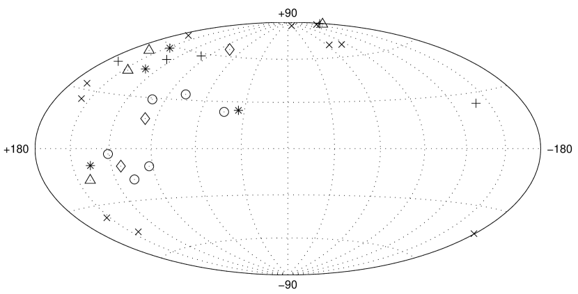
Table 1 lists the objects whose observations are reported here. In the table, we provide the object name (or names), its equatorial coordinates, its redshift and classification. The locations of these BL Lacs, along with those of 1ES 2344+514, H 1426+428 and 1ES 1959+650, are plotted in Galactic co-ordinates in Figure 1.

The majority of the objects in Table 1 were selected for observations as part of three BL Lac campaigns. The first was a survey of all known (circa 1995) BL Lac objects with redshift of $\lesssim 0.1$ . The goal was to investigate the intrinsic characteristics of BL Lac objects that led to the production of TeV gamma rays. We selected low redshift objects to minimize the effect of the attenuation of the VHE gamma-ray signal by pair production with extragalactic background light (Stecker, 1999; Primack et al., 1999; Vassiliev, 2000) so that the intrinsic features could be compared. The second campaign was to search for TeV emission from HBLs in the redshift range from 0.1 to 0.2. We believed that because the HBLs have SEDs similar to the confirmed TeV emitters that they would be stronger TeV candidates than the LBLs. Because of the potential attenuation by the EBL and the larger pool of objects in the z=0.1-0.2 range, we needed to be more selective in our surveys. The third campaign was a “snapshot survey” (D’Vali et al., 1999) in which many BL Lacs which were considered likely candidates for TeV emission based on the same criteria as the second survey were observed. When in a flaring state, a 10 minute observation of Mrk 421 or Mrk 501 was enough to achieve a significant detection. The selected snapshot survey targets were therefore observed for 10 minutes each on a regular basis in the hope of catching one of them in such a flaring state. The objects were grouped based upon their proximity to each other on the celestial sphere. Objects in each group were then observed consecutively so as to minimize telescope slewing time. The remaining objects with known redshift were chosen because they were EGRET sources (W Comae, PKS 0829+046, S4 0954+65, 3C 66A) or because they were a superluminal source (OQ 530). RGB J1725+118 (4U 1722+11) was observed because one measurement (Veron-Cetty & Veron, 1993) derived a redshift of $z=0.018$ , which would make it the closest known BL Lac object. The estimate was however, derived from one absorption line and many papers list its redshift as unknown (e.g., Padovani & Giommi, 1995b).

3 Analysis Methods

3.1 Telescope Configurations

The VHE observations reported in this paper were made with the atmospheric Cherenkov imaging technique (Cawley & Weekes, 1995; Reynolds et al., 1993) using the 10-m optical reflector located at the Whipple Observatory on Mt. Hopkins in Arizona (elevation 2.3 km) (Cawley et al., 1990). A camera, consisting of an array of photomultiplier tubes (PMTs) mounted in the focal plane of the reflector, records images of atmospheric Cherenkov radiation from air showers produced by gamma rays and cosmic rays. The observations reported here span five years and the camera of the Whipple gamma-ray telescope changed several times during that period. Table 2 outlines the configurations of the camera. Light concentrators are reflective cones that are mounted in front of the PMTs to improve light collection efficiency and reduce albedo. During 1999, an intelligent trigger “the Pattern Selection Trigger” (PST) (Bradbury et al., 1999) was installed that required three adjacent tubes to record a signal above a certain level within a preset window. Prior to this, a trigger was declared if any two PMTs in the camera recorded a signal above a certain level within a preset window. The PST reduces the number of triggers caused by fluctuations of the night-sky background and thus allows the telescope to operate at lower energies. The mirror reflectivity and trigger settings also changed over time. Each observing season runs approximately from September through June. Observations are not usually carried out in July and August because the monsoon season, during which lightning storms strike frequently, occurs at this time.

3.2 Gamma-ray Selection

We characterize each Cherenkov image using a moment analysis (Reynolds et al., 1993). The roughly elliptical shape of the image is described by the length and the width parameters, and its location and orientation within the telescope field of view are given by the distance and $\alpha$ parameters, respectively. We also determine the two highest signals recorded by the PMTs (max1, max2) and the amount of light in the image size. In addition, we can apply a cut on the third moment parameter asymmetry to select gamma-ray candidates since the narrower tail of the image should point back toward the source location within the FOV. The $\alpha$ parameter tests whether the major axis of the image is aligned with the putative source location; it does not eliminate events whose major axes are parallel with the source location but whose image points away from it. The asymmetry parameter is not an efficient cut for cameras with small fields of view because the images are often truncated.

Because of the changes in the camera discussed above in Section 3.1, the optimum cuts for selecting gamma rays change with time. The cuts for different camera configurations are listed in Table 3. They result in different sensitivities, energy ranges, and effective areas for each camera. This limits our ability to combine data from different observing periods into single upper limits. Given the variable nature of BL Lac objects however, deriving single upper limits for several years of observation is of dubious benefit. Instead we quote upper limits for each observing period.

3.3 Tracking Analysis

The observations presented here were all taken in the Tracking data collection mode wherein only the on-source position is tracked, in runs of 28 minute duration. To estimate the expected background, we use those events that pass all of the gamma-ray selection criteria except orientation (characterized by the $\alpha$ parameter). We use events with values of $\alpha$ between 20^∘ and 65^∘ as the background region and convert the counts to an estimated background within the on-source region ( $\alpha<10^{\circ}$ or $15^{\circ}$ ; see Table 3) by multiplying the number of counts by a ratio determined from observations of non-source regions taken at other times during the observing season. This method has been described in detail by Catanese et al. (1998). The value of the factor that converts the off-source counts to an on-source background estimate varies with season due to changes in the camera sensitivity and field of view. The estimated values for each of the observing periods are listed in Table 4.

In the case of tracking analysis, to establish the significance (S) of an excess or of a deficit, we use simple error propagation:

S={{N_{\rm on}-r*N_{\rm bkd}}\over{\sqrt{N_{\rm on}+r^{2}*N_{\rm bkd}+N_{\rm bkd}^{2}*(\Delta r)^{2}}}}

(1)

where $N_{\rm on}$ is the number of events in the on-source region (designated by the $\alpha$ cut in Table 3), $N_{\rm bkd}$ is the number of events in the background region ( $\alpha=20^{\circ}-65^{\circ}$ ), and $r\pm\Delta r$ is the tracking ratio and its statistical uncertainty.

3.4 Flux Upper Limit Estimation

After we select gamma-ray candidate events, we determine the significance of any excess or deficit in the observations. If the excess or the deficit is not statistically significant, as is the case for all observations reported here, we calculate a 99.9% confidence level (C.L.) upper limit on the count rate by using the method of Helene (1983). To convert these flux upper limits to absolute fluxes, we first express them as a fraction of the Crab Nebula count rate by using observations from the same observing period. Although this method assumes a Crab-like spectrum for the BL Lacs, it corrects for season to season variations in factors like PMT gain and mirror reflectivity which affect the telescope response, and therefore its gamma-ray count rate. The count rates observed for the Crab Nebula for the observing periods reported here are given in Table 4. Analysis of the Crab Nebula data shows that for runs taken under good weather conditions, the gamma-ray count rate does not change significantly within a season (Quinn, 1998). We can therefore assume that the gamma-ray count rate for a source can be reliably expressed in terms of the Crab Nebula flux over the course of the season.

Once we have the flux limit expressed as a fraction of the Crab Nebula count rate, we multiply it by the integral Crab Nebula flux (in units of photons cm^-2 s^-1) above the peak response energy of the observations (E_p). We define E_p as the energy at which the collection area folded with an E^-2.5 spectrum, that of the Crab Nebula (Hillas et al., 1998), reaches a maximum. The integral fluxes from the Crab Nebula above E_p for the different observations periods reported here are given in Table 4. Upper limits are an estimate of the flux that could be present in the data set but not produce a significant excess. This is most accurately derived from the count rate because that is what determines the statistical significance of the excess. The Crab Nebula count rate and flux uncertainties affect only the normalization, so the flux upper limits quoted in terms of photons cm^-2 s^-1 have an uncertainty of $\sim$ 25%, mainly from the uncertainty in the Crab Nebula photon flux.

4 Results and Discussion

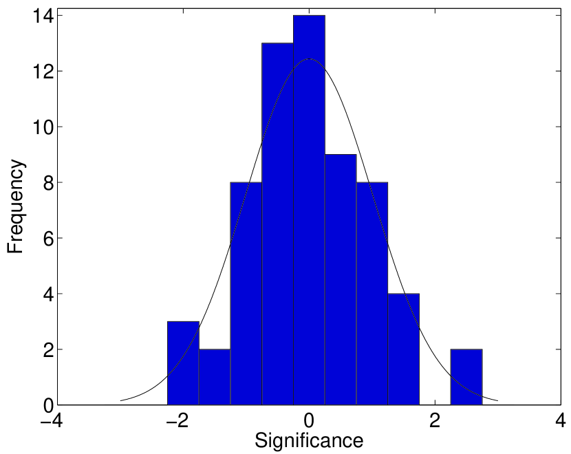
Table 5 summarizes the results of the observations of the BL Lacs observed but not detected between January 1995 and July 2000 while Table 6 summarizes the results of the observations taken on H1426+428, 1ES1959+650 and 1ES2344+514, the three BL Lacs that were detected during this survey. For each target object, we list the observation exposure during each season, the significance of the excess or deficit of these observations, the maximum significances for a night or month of observations and the flux upper limits expressed as fractions of the Crab count rate and in integral flux units (assuming a Crab-like spectrum). Many of the objects were observed over a number of different observing seasons resulting in a range of upper limits above different values of E_p. No evidence for a statistically significant excess or deficit was seen in the detected count rate from any of the objects for any of the time periods examined. The distribution of the significances for each object for each observing season is shown in Figure 2. This distribution has a mean of 0.005 with a standard deviation of 0.976. The black curve shows the expected shape if the significances were drawn from a Gaussian distribution. The Kolmogorov-Smirnov test returns a 95% probability that the data are normally distributed.

Table 8 summarizes the detections of H1426+428, 1ES1959+650 and 1ES2344+514, the three target BL Lacs that have been subsequently confirmed as TeV emitters.

In order to investigate how much the flux upper limits change if the spectral index is not the same as that of the Crab Nebula, estimates of the flux upper limits for the BL Lacs were made assuming source spectral indices of -2.2 and -2.8. The integral flux from the Crab Nebula above 300 GeV was used to scale the previously calculated upper limits. This integral flux was assumed to remain constant when the spectral index was changed. E_p was not adjusted to account for the response of the telescope to the different input spectra but this effect should be very small. Table 7 lists the flux upper limits for each BL Lac for each observing season when these different source spectral indices were assumed.

Costamante & Ghisellini (2002) have made predictions for the TeV flux from fourteen of the BL Lacs included in this paper using two different methods. In the first, an SSC model was used to fit the multiwavelength data gathered on each of the objects while in the second approach, a phenomenological description of the average SED of the blazars was derived based upon their observed bolometric luminosity (Fossati et al., 1998). The resulting flux predictions from each of the two methods were given above 300 GeV and above 1 TeV. In order to compare the upper limits presented here with these predictions, our upper limits that were not already derived above 300 GeV, were extrapolated to this energy. This was done by first expressing the flux upper limit as a fraction of the Crab flux at that energy, F_BLLac( $>E_{p}$ ). This was then scaled to 300 GeV assuming a Crab-like spectrum. Thus, an upper limit on the integral flux for each BL Lac above 300 GeV for each observing season, F_BLLac( $>$ 300GeV), was calculated:

F_{BLLac}(>300GeV)=F_{BLLac}(>E_{p})\,F_{Crab}(>E_{p})\left({\displaystyle\frac{300}{E_{p}}}\right)^{-1.5}

(2)

F_Crab( $>$ E_p) is the integral flux from the Crab Nebula above E_p in units of photons cm^-2 s^-1, assuming an integral spectral index of -1.5. F_BLLac( $>E_{p}$ ) is the upper limit on the flux from the BL Lac above E_p expressed as a fraction of the Crab Nebula integral flux at this energy.

When deriving their flux predictions, Costamante & Ghisellini (2002) did not take into account absorption of the gamma rays by the infra-red background. The predictions above 300 GeV could therefore change by factors on the order of 5 for objects at redshifts above 0.2. The upper limits presented here were compared with these predictions and, those of four BL Lacs, shown in Table 9, were found, during all seasons in which they were observed, to be lower than the predicted fluxes according to the Fossati approach (Fossati et al., 1998) adapted in (Costamante & Ghisellini, 2002). Those of two more BL Lacs, also listed in Table 9, were found to be lower during some of the observing periods. All of the upper limits calculated were higher than the fluxes predicted using the one-zone, SSC model (Costamante & Ghisellini, 2002). It should be noted however, that the upper limits quoted here pertain only to the specific period during which the observations were made. As demonstrated by Bottcher et al. (2002), spectral fitting of blazars is subject to very large uncertainties when non-simultaneous multiwavelength data are used. Indeed, it is also shown that, even with the best currently available simultaneous optical - X-ray data, there is a very wide range in the predicted fluxes above 40 GeV. Given an observed X-ray flux, the predicted gamma-ray flux depends very sensitively on the model parameters and, even for simultaneous data, can vary by large factors due to the uncertainty in these parameters.

In the absence of dedicated simultaneous multiwavelength data, it is difficult to use these data to constrain emission models. However, many of the objects surveyed here are monitored by the All Sky Monitor (ASM) on board the Rossi X-ray Timing Explorer. For many other TeV blazars, the soft X-ray flux has been seen to rise during periods when the gamma-ray flux was also high. For example, Mrk 501 was observed to have a higher than average flux in the ASM during 1997, the same year during which the greatest TeV flaring activity detected to date was observed (Catanese et al., 1997b; Quinn et al., 1999). In order to see if any of the BL Lacs surveyed here were particularly active in the X-ray band during these observations, the X-ray curves for the objects presented here that are monitored by ASM were analyzed. If heightened X-ray activity was detected in the absence of corresponding gamma-ray activity, this could have interesting consequences for emission models. Out of the 29 objects presented here, 25 of them are monitored on a regular basis by the ASM. The nightly average light curves for each of these were generated. The flux from each object was found to be, on average, very low ( $\lesssim$ 0.01 Crab units ) with no evidence for dramatic flaring or for any sustained period of X-ray activity.

Current and future observing campaigns at the Whipple Observatory make use of BL Lac monitoring at X-ray wavelengths to try to predict when an object might be in a higher flux state and thus detectable in the VHE band. Elevated gamma-ray fluxes are often accompanied by a corresponding increase in the X-ray flux (e.g. Maraschi et al., 1999; Jordan et al., 2001). Thus, by monitoring the X-ray activity from blazars, we can identify periods of increased activity during which the VHE flux may also be stronger. However, the relationship between the X-ray and gamma-ray flux has been shown to be complicated with gamma-ray flares being detected in the absence of X-ray flares (Holder et al., 2003; Krawczynski et al., 2003), and vice-versa (Rebillot et al., 2003).

Finally, it should be noted that, although none of the objects presented here were found to have a statistically significant TeV flux during these observations, three of the confirmed TeV blazars were detected during this survey. When 1ES2344+514, H1426+428 and 1ES1959+650 were initially observed at Whipple, it was as part of this BL Lac campaign and, like the objects listed here, they were not detected. In subsequent years however, continued monitoring with deeper exposures revealed these objects to be TeV emitters when in more active states, although not always detectable when in their quiescent state. Continued VHE observations of the BL Lacs presented here, in particular those shown to have extreme properties (de la Calle Perez et al., 2003), accompanied by monitoring of their X-ray flux level, may reveal many more of them to be TeV emitters. Indeed, since extreme BL Lacs, the best blazar candidates for TeV emission, have lower luminosity at all wavelengths than their lower energy peaked counterparts, their flux level often lies below the detection threshold of the current generation of imaging atmospheric Cherenkov telescopes when they are in quiescent state. As the next generation of ground-based gamma-ray telescopes comes online with their increased flux sensitivity, they will offer a unique opportunity to study this low luminosity class of blazar and should detect many more of these objects.

Future, X-ray all-sky monitor experiments like LOBSTER (Black et al., 2003) and EXIST (Grindlay et al., 2002), with their improved flux sensitivity and increased bandwidth, will allow for more detailed monitoring of the X-ray emission from blazars thus providing valuable information which can be used to trigger observations at gamma-ray energies. These X-ray missions, coupled with the next generation of higher sensitivity VHE observatories such as VERITAS, HESS, MAGIC and CANGAROO, should allow both lower power extreme BL Lacs and lower frequency peaked blazars (LBLs and FSRQs) to be detected.

We acknowledge the technical assistance of E. Roache and J. Melnick. We also thank the anonymous referee for his/her comments which enabled us to improve this paper. This research is supported by grants from the U. S. Department of Energy, the National Science Foundation, by Enterprise Ireland and by PPARC in the UK. This research has made use of the NASA/IPAC Extragalactic Database (NED) which is operated by the Jet Propulsion Laboratory, California Institute of Technology, under contract with the National Aeronautics and Space Administration. This research made use of the quick-look results provided by the ASM/RXTE team.

References

Aharonian et al. (2000) Aharonian, F. A., et al. 2000, A&A, 353, 847
Black et al. (2003) Black, J. K., Brunton, A. N., Bannister, N. P., Deines-Jones, P. & Jahoda K. 2003, to be published in NIM A (astro-ph/0305025)
Blandford & Levinson (1995) Blandford, R. D. & Levinson, A. 1995, ApJ, 441, 79
Bloom & Marscher (1996) Bloom, S. D., & Marscher, A. P. 1996, ApJ, 461, 657
Bottcher et al. (2002) B $\ddot{o}$ ttcher, M., Muckherjee, R. & Reimer, A. 2002, ApJ, 581, 143
Bradbury et al. (1999) Bradbury, S. M., Burdett, A. M., D’Vali, M., Ogden, P. A., & Rose, H. J. 1999, AIP Conf. Proc. 516, Proceedings of the 26th International Cosmic Ray Conference, ed. B. L. Dingus, D. B. Kieda & M. H. Salamon (Salt Lake City, Utah:AIP), 5, 263
Buckley (1998) Buckley, J. H. 1998, Science, 279, 676
Caccianiga et al. (1999) Caccianiga, A., Maccacaro, T., Wolter, A., della Ceca, R., & Gioia, I. M. 1999, ApJ, 513, 51
Catanese et al. (1997a) Catanese, M., et al. 1997, in Proceedings of the Fourth Compton Symposium, ed. C. D. Dermer, M. S. Strickman, & J. D. Kurfess (New York: AIP), AIP Conf. Proc., 410, 1376
Catanese et al. (1997b) Catanese, M., et al. 1997b, ApJ, 487, L143
Catanese et al. (1998) Catanese, M., et al. 1998, ApJ, 501, 616
Cawley et al. (1990) Cawley, M. F., et al. 1990, Exp. Astron., 1, 173
Cawley & Weekes (1995) Cawley, M. F., & Weekes, T. C. 1995, Exp. Astron., 6, 7
Chadwick et al. (1999) Chadwick, P. M., et al. 1999, ApJ, 521, 547
Costamante & Ghisellini (2002) Costamante, L. & Ghisellini, G. 2002, A&A, 384, 56
de la Calle Perez et al. (2003) de la Calle Perez, I., et al. 2003, preprint (astro-ph/0309063)
Dermer, Schlickeiser & Mastichiadis (1992) Dermer, C. D., Schlickeiser, R., & Mastichiadis, A. 1992, A&A, 256, L27
Dermer & Schlickeiser (1993) Dermer, C. D. & Schlickeiser, R. 1993, ApJ, 416, 458
Dermer & Schlickeiser (1994) Dermer, C. D., & Schlickeiser, R. 1994, ApJs, 90, 945
Dermer & Davis (2000) Dermer, C. D. & Davis, S. P. 2000, AIP Conf. Proc. 520, 1, 425
Djannati-Atai et al. (2003) Djannati-Atai, A., et al. 2003, Proc. 28th International Cosmic Ray Conference, Tsukuba, Japan
D’Vali et al. (1999) D’Vali, M., et al. 1999, Proceedings.of the 26th International Cosmic Ray Conference, ed. B. L. Dingus, D. B. Kieda & M. H. Salamon, (Salt Lake City, U. S. A.), 26, 422
Fossati et al. (1997) Fossati, G., Celotti, A., Ghisellini, G. & Maraschi, L., 1997, MNRAS, 289, 136
Fossati et al. (1998) Fossati, G., Maraschi, L., Celotti, A., Comastri, A. & Ghisellini, G. 1998, MNRAS, 299, 433
Ghisellini & Madau (1996) Ghisellini, G. & Madau, P. 1996, MNRAS, 280, 67
Ghisellini et al. (1998) Ghisellini, G., Celotti, A., Fossati, G., Maraschi, L., & Comastri, A. 1998, MNRAS, 301, 451
Ghisellini (1999) Ghisellini, G. 1999, Astropart. Phys., 11, 11
Grindlay et al. (2002) Grindlay, J. E., Craig, W. W., Geherls, N., Harrison, F. A. & Hong, J. 2002, to appear in Proc. SPIE, vol. 4851
Hartman et al. (1999) Hartman, R. C., et al. 1999, ApJs, 123, 79
Helene (1983) Helene, O. 1983, Nucl. Instrum. Methods Phys. Res., 212, 319
Hillas et al. (1998) Hillas, A. M., et al. 1998, ApJ, 503, 744
Holder et al. (2003) Holder, J., et al.. 2003, ApJ, 583, L9
Horan et al. (2000) Horan D., et al. 2000, HEAD Meeting, (Honolulu, Hawaii), No. 32, 05.03
Horan et al. (2002) Horan, D., et al. 2002, ApJ, 571, 753
Horan et al. (2003) Horan, D., et al. 2003, to be published in the Proceedings of the 2nd VERITAS Symposium on TeV Astrophysics of Extragalactic Sources” (Chicago)
Jordan et al. (2001) Jordan, M., et al. 2001, Proceedings of the 27th International Cosmic Ray Conference, (Hamburg, Germany), 7, 2691
Kerrick et al. (1995) Kerrick, A. D., et al. 1995, ApJ, 452, 588
Königl (1981) Königl, A. 1981, ApJ, 243, 700
Krawczynski et al. (2003) Krawczynski H., et al. 2003, in press
Laurent-Muehleisen et al. (1999) Laurent-Muehleisen, S. A., Kollgaard, R. I., Feigelson, E. D., Brinkmann, W., Siebert, J. 1999, ApJ, 525, 127
Mannheim (1998) Mannheim, K. 1998, Science, 279, 684
Maraschi, Ghisellini & Celotti (1992) Maraschi, L., Ghisellini, G., & Celotti, A. 1992, ApJ, 397, L5
Maraschi et al. (1999) Maraschi, L., et al. 1999, Astropart. Phys., 11, 189
Mucke et al. (2003) M $\ddot{u}$ cke, A., et al. 2003, Astropart. Phys., 18, 593
Neshpor et al. (1998) Neshpor, Y. I., et al. 1998, Astron. Letts., 24, 134
Neshpor et al. (2001) Neshpor, Y. I, Chalenko, N. N, Stepanian, A. A., Kalekin, O. R, Jogolev, N. A, Fomin, V. P., & Shitov, V. G. 2001, Astronomy Reports, 45, 249
Nishiyama et al. (2000) Nishiyama, T., et al. 2000, AIP Conf. Proc. 516, Proceedings of the 26th International Cosmic Ray Conference, ed. B. L. Dingus, D. B. Kieda & M. H. Salamon (Salt Lake City, Utah:AIP), 3, 370
Padovani & Giommi (1995a) Padovani, P. & Giommi, P. 1995, ApJ, 444, 567
Padovani & Giommi (1995b) Padovani, P., & Giommi, P. 1995b, MNRAS, 277, 1477
Perlman et al. (1998) Perlman, E. S., Padovani, P., Giommi, P., Sambruna, R., Jones, L. R., Tzioumis, A., & Reynolds, J. 1998, AJ, 115, 1253
Primack et al. (1999) Primack, J. R., Bullock, J. S., Somerville, R. S., MacMinn, D. 1999, Astropart. Phys., 11, 93
Punch et al. (1992) Punch, M., et al. 1992, Nature, 358, 477
Quinn et al. (1996) Quinn, J. et al. 1996, ApJ, 456, L83
Quinn (1998) Quinn, J. 1998, Ph.D. Thesis, National University of Ireland
Quinn et al. (1999) Quinn, J., et al. 2000, ApJ, 518, 693
Rebillot et al. (2003) Rebillot, P., et al. 2003, Proc. 28th International Cosmic Ray Conference, Tsukuba, Japan, 2599
Reynolds et al. (1993) Reynolds, P. T., et al. 1993, ApJ, 404, 206
Roberts et al. (1998) Roberts, M. D., et al. 1998, A&A, 337, 25
Roberts et al. (1999) Roberts, M. D., et al. 1999, A&A, 343, 691
Sikora et al. (1994) Sikora, M., Begelman, M. C. & Rees, M. J. 1994, ApJ, 421, 153
Sikora & Madejski (2001) Sikora, M. & Madejski, G. 2001, AIP Proc. 558, 275
Stecker (1999) Stecker, F. W. 1999, Astropart. Phys., 11, 83
Tagliaferri et al. (2000) Tagliaferri, G., et al. 2000, A&A, 354, 431
Tluczykont et al. (2003) Tluczykont, M., et al. 2003, Proc. 28th International Cosmic Ray Conference, Tsukuba, Japan, 2547
Urry & Padovani (1995) Urry, C. M. & Padovani, P. 1995, Publications of the Astronomical Society of the Pacific, 107, 803
Vassiliev (2000) Vassiliev, V. V. 2000, Astropart. Phys., 12, 217
Veron-Cetty & Veron (1993) Veron-Cetty, M. P., & Veron, P. 1993, A&AS, 100, 521
Wagner et al. (1995) Wagner, S. J., et al. 1995, A&A, 298, 688

Table 1: Observed BL Lac Objects

Name	(J2000)	(J2000)	$z$	Class^a^aHBL = high-frequency-peaked BL Lac object; LBL = low-frequency-peaked BL Lac object.
	R.A.	Dec.
1ES 0033+595	00 35 52.6	+59 50 05	0.086	HBL
1ES 0145+138	01 48 29.7	+14 02 18	0.125	HBL
RGB J0214+517	02 14 17.9	+51 44 52	0.049	HBL
3C 66A, 1ES 0219+428^c,d^c,dfootnotemark:	02 22 39.6	+43 02 08	0.444	LBL
1ES 0229+200	02 32 48.4	+20 17 16	0.140	HBL
1H 0323+022, 1ES 0323+022	03 26 14.0	+02 25 15	0.147	HBL
EXO 0706.1+5913, RGB J0710+591	07 10 30.0	+59 08 20	0.125	HBL
1ES 0806+524	08 09 49.1	+52 18 59	0.138	HBL
PKS 0829+046, RGB J0831+044^d^dEGRET source of $>$ 100 MeV gamma rays.	08 31 48.9	+04 29 39	0.180	LBL
1ES 0927+500	09 30 37.6	+49 50 26	0.188	HBL
S4 0954+65, RGB J0958+655^d^dEGRET source of $>$ 100 MeV gamma rays.	09 58 47.2	+65 33 55	0.368	LBL
1ES 1028+511	10 31 18.4	+50 53 36	0.361	HBL
1ES 1118+424	11 20 48.0	+42 12 12	0.124	HBL
Markarian 40	11 25 36.2	+54 22 57	0.021	HBL
Markarian 180, 1ES 1133+704	11 36 26.4	+70 09 27	0.045	HBL
1ES 1212+078	12 15 10.9	+07 32 04	0.130	HBL
ON 325, 1ES 1215+303	12 17 52.1	+30 07 01	0.130	LBL
1H 1219+301, 1ES 1218+304	12 21 21.9	+30 10 37	0.182	HBL
W Comae, 1ES 1218+285^d^dEGRET source of $>$ 100 MeV gamma rays.	12 21 31.7	+28 13 59	0.102	LBL
MS 1229.2+6430, RGB J1231+642	12 31 31.4	+64 14 18	0.170	HBL
1ES 1239+069	12 41 48.3	+06 36 01	0.150	HBL
1ES 1255+244	12 57 31.9	+24 12 40	0.141	HBL
OQ 530, RGB J1419+543	14 19 46.6	+54 23 15	0.151	LBL
4U 1722+11, RGB J1725+118^b^bThis object is sometimes quoted as having a redshift of 0.018. However, this is based on one absorption line (Veron-Cetty & Veron, 1993) and is more commonly listed as having an unknown redshift.	17 25 04.3	+11 52 15	0.018	HBL
I Zw 187, 1ES 1727+502	17 28 18.6	+50 13 10	0.055	HBL
1ES 1741+196	17 43 57.8	+19 35 09	0.084	HBL
3C 371, 1ES 1807+698	18 06 50.6	+69 49 28	0.051	LBL
BL Lacertae, 1ES 2200+420^d^dEGRET source of $>$ 100 MeV gamma rays.	22 02 43.3	+42 16 40	0.069	LBL
1ES 2321+419	23 23 52.1	+42 10 59	0.059	HBL

^c^cfootnotetext: Unconfirmed source of TeV gamma rays.

Table 2: Whipple Camera Configurations

	1995/01-	1997/01-	1997/09-	1998/12-	1999/10-
Period	1996/12	1997/06	1998/12	1999/03	2000/07
Number of PMTs	109	151	331	331	379^a^aThe camera consists of 379 inner tubes of FOV 0 $\fdg$ 12 diameter surrounded by three circular rings of PMTs (111 in all) of FOV 0 $\fdg$ 26 diameter. The outer rings of tubes were not used in this analysis and so, the parameters presented here pertain only to the inner 379 tubes.
PMT spacing	0 $\fdg$ 259	0 $\fdg$ 259	0 $\fdg$ 24	0 $\fdg$ 24	0 $\fdg$ 12
Field of View	3^∘	3 $\fdg$ 3	4 $\fdg$ 8	4 $\fdg$ 8	2 $\fdg$ 6
Light concentrators	yes	yes	no	yes	yes
Pattern trigger	no	no	no	no	yes

Table 3: Analysis Cuts

	1995/01-	1997/01-	1997/09-	1998/12-	1999/10-
Period	1996/12	1997/06	1998/12	1999/03	2000/07
max1^a^aQuantities are in units of digital counts (d.c.): 1 d.c. $\approx$ 1 photoelectron.	$>$ 100	$>$ 95	$>$ 60	$>$ 60	$>$ 30
max2^a^aQuantities are in units of digital counts (d.c.): 1 d.c. $\approx$ 1 photoelectron.	$>$ 80	$>$ 45	$>$ 40	$>$ 40	$>$ 30
size^a^aQuantities are in units of digital counts (d.c.): 1 d.c. $\approx$ 1 photoelectron.	$>$ 400	N.A.^b^bN.A. means the cut was not applied.	N.A.	N.A.	N.A.
length	$>0\fdg 16$	$>0\fdg 16$	$>0\fdg 16$	$>0\fdg 16$	$>0\fdg 13$
	$<0\fdg 30$	$<0\fdg 33$	$<0\fdg 50$	$<0\fdg 50$	$<0\fdg 25$
width	$>0\fdg 073$	$>0\fdg 073$	$>0\fdg 073$	$>0\fdg 073$	$>0\fdg 05$
	$<0\fdg 15$	$<0\fdg 16$	$<0\fdg 16$	$<0\fdg 16$	$<0\fdg 12$
distance	$>0\fdg 51$	$>0\fdg 51$	$>0\fdg 51$	$>0\fdg 51$	$>0\fdg 40$
	$<1\fdg 10$	$<1\fdg 17$	$<1\fdg 55$	$<1\fdg 55$	$<1\fdg 00$
alpha	$<15^{\circ}$	$<15^{\circ}$	$<15^{\circ}$	$<15^{\circ}$	$<15^{\circ}$
asymmetry	N.A.	$>0^{\circ}$	$>0^{\circ}$	$>0^{\circ}$	$>0^{\circ}$
length over size	N.A.	N.A.	N.A.	N.A.	$<0.0004$

Table 4: Analysis Parameters

	Tracking	Crab rate	Peak Response	Integral
Period	Ratio	( $\gamma$ /min)	Energy	Crab flux^a^aFluxes are quoted in units of 10^-10 photons cm^-2 s^-1 above the corresponding peak response energy.
1995/01 - 1995/08	0.292 $\pm$ 0.005	2.08 $\pm$ 0.15	300 GeV	1.26
1995/10 - 1996/07	0.292 $\pm$ 0.004	1.58 $\pm$ 0.05	350 GeV	1.05
1996/10 - 1996/12	0.316 $\pm$ 0.004	1.69 $\pm$ 0.07	350 GeV	1.05
1997/01 - 1997/06	0.345 $\pm$ 0.005	2.30 $\pm$ 0.10	350 GeV	1.05
1998/01 - 1998/12	0.366 $\pm$ 0.002	1.94 $\pm$ 0.15	500 GeV	0.60
1998/12 - 1999/03	0.367 $\pm$ 0.004	2.62 $\pm$ 0.26	400 GeV	0.84
1999/10 - 2000/07	0.312 $\pm$ 0.002	2.64 $\pm$ 0.12	430 GeV	0.76

Table 5: The observation results for each object, for each observing period during which it was observed. For each BL Lac, the total combined significance for each period is given along with the maximum statistical significance seen over any one night and any month during that period. The flux upper limits are also presented for each observing period both in absolute terms (Flux units, f.u., 10^-11 cm^-2 s^-1) and in Crab units (c.u.).

	Observation	Exp.		Max. $\sigma$	Max. $\sigma$	Flux	Flux
Object	Period	(hrs)	$\sigma$	Month	Night	(c.u.)	(f.u.)
1ES 0033+595	1995/12	1.85	-0.59	-0.59	0.19	$<$ 0.200	$<$ 2.10
1ES 0145+138	1996/10 - 1996/11	7.85	-1.01	0.08	1.77	$<$ 0.093	$<$ 0.98
	1998/11 - 1998/12	2.29	0.22	0.63	0.63	$<$ 0.512	$<$ 3.50
	1998/12 - 1999/01	1.98	-0.50	0.38	1.31	$<$ 0.357	$<$ 3.34
RGB J0214+517	1999/12 - 2000/01	6.01	0.29	0.36	1.58	$<$ 0.165	$<$ 1.45
3C 66A	1995/10 - 1995/11	8.00	-2.00	-1.18	0.82	$<$ 0.056	$<$ 0.59
1ES 0229+200	1996/11 - 1996/12	7.85	0.15	0.57	1.37	$<$ 0.113	$<$ 1.19
	1998/11 - 1998/12	2.30	-1.08	-0.78	0.48	$<$ 0.326	$<$ 2.23
	1998/12 - 1999/01	1.78	-0.40	0.66	0.74	$<$ 0.403	$<$ 3.76
1H 0323+022	1996/11 - 1996/12	10.18	1.02	1.02	1.96	$<$ 0.181	$<$ 1.90
	1997/01	0.91	0.20	0.20	0.20	$<$ 0.298	$<$ 3.13
	1998/12 - 1999/01	3.18	1.69	1.73	1.85	$<$ 0.509	$<$ 4.75
EXO 0706.1+5913	1996/12	5.55	-1.16	-1.16	0.17	$<$ 0.087	$<$ 0.91
	1997/01 - 1997/03	3.69	0.76	0.79	1.46	$<$ 0.161	$<$ 1.69
	1998/11	1.83	-0.40	-0.40	1.49	$<$ 0.524	$<$ 3.58
	1998/12 - 1999/02	1.90	0.07	1.36	1.71	$<$ 0.459	$<$ 4.29
1ES 0806+524	1996/02 - 1996/03	5.57	0.46	0.52	1.04	$<$ 0.104	$<$ 1.09
	2000/01 - 2000/03	4.16	-0.29	0.69	0.69	$<$ 1.293	$<$ 11.4
PKS 0829+046	1995/01 - 1995/04	11.07	1.25	1.73	3.14	$<$ 0.117	$<$ 1.47
1ES 0927+500	1996/12	5.08	-1.92	-1.92	0.39	$<$ 0.064	$<$ 0.67
	1997/01 - 1997/04	5.04	-1.03	0.22	1.23	$<$ 0.076	$<$ 0.80
S4 0954+65	1995/02 - 1995/03	3.70	-1.09	-0.50	-0.11	$<$ 0.096	$<$ 1.21
1ES 1028+511	1998/12 - 1999/02	4.43	0.57	1.36	2.03	$<$ 0.287	$<$ 2.68
1ES 1118+424	1998/02 - 1998/04	7.30	-0.25	1.29	1.80	$<$ 0.218	$<$ 1.49
	1998/12 - 1999/02	3.60	0.27	1.04	1.81	$<$ 0.310	$<$ 2.90
	2000/01 - 2000/05	6.97	-0.62	1.29	1.61	$<$ 0.116	$<$ 1.02
Markarian 40	2000/01 - 2000/04	10.16	2.59	1.66	1.56	$<$ 0.206	$<$ 1.81
Markarian 180	1995/01 - 1995/04	5.55	-0.10	0.45	1.07	$<$ 0.108	$<$ 1.36
	1995/12 - 1996/05	20.46	-0.26	1.01	1.70	$<$ 0.105	$<$ 1.10
	1997/01	0.79	-0.17	-0.17	-0.17	$<$ 0.303	$<$ 3.18
1ES 1212+078	1999/02	1.13	0.44	0.44	1.83	$<$ 0.778	$<$ 7.26
	2000/01 - 2000/05	3.70	1.30	1.52	1.73	$<$ 0.321	$<$ 2.82
ON 325	1999/02	0.97	1.27	1.27	1.20	$<$ 0.882	$<$ 8.23
	2000/01 - 2000/05	5.05	0.88	1.94	1.62	$<$ 0.215	$<$ 1.89
1H 1219+301	1995/01 - 1995/05	2.77	2.71	2.90	2.95	$<$ 0.226	$<$ 2.85
	1997/02 - 1997/06	11.27	0.99	1.55	1.97	$<$ 0.079	$<$ 0.83
	1998/01 - 1998/03	1.38	-1.96	-1.27	-0.32	$<$ 0.356	$<$ 2.43
	1998/12 - 1999/02	2.94	-0.08	0.48	0.88	$<$ 0.296	$<$ 2.77
	2000/01 - 2000/04	3.69	0.04	1.48	1.18	$<$ 0.191	$<$ 1.68
W Comae	1995/02 - 1995/04	14.33	-0.57	-0.11	1.14	$<$ 0.052	$<$ 0.66
	1996/01 - 1996/05	15.73	-0.29	0.24	1.38	$<$ 0.055	$<$ 0.58
	1999/01 - 1999/02	4.43	-0.03	0.58	1.91	$<$ 0.312	$<$ 2.92
	2000/01 - 2000/04	4.72	-0.58	1.01	1.76	$<$ 0.148	$<$ 1.30
MS 1229.2+6430	1995/02 - 1995/04	1.39	1.32	1.08	1.08	$<$ 0.286	$<$ 3.60
	1999/02	2.04	-0.76	-0.76	1.18	$<$ 0.446	$<$ 4.16
	2000/01 - 2000/05	6.01	0.35	1.72	1.72	$<$ 0.170	$<$ 1.50
1ES 1239+069	1999/01 - 1999/02	1.73	0.78	0.69	1.74	$<$ 0.616	$<$ 6.04
	2000/01 - 2000/05	5.08	0.11	1.19	1.42	$<$ 0.197	$<$ 1.73
1ES 1255+244	1997/02 - 1997/05	5.54	1.19	1.01	1.35	$<$ 0.112	$<$ 1.18
	1998/03	0.46	0.13	0.13	0.13	$<$ 1.112	$<$ 7.60
	1999/02	1.73	0.15	0.15	1.10	$<$ 0.508	$<$ 4.75
	2000/01 - 2000/05	4.16	-0.54	1.30	1.41	$<$ 0.164	$<$ 1.45
OQ 530	1995/03 - 1995/05	7.39	-0.73	-0.15	0.76	$<$ 0.058	$<$ 0.73
4U 1722+11	1995/04 - 1995/05	2.77	-0.08	0.28	0.70	$<$ 0.124	$<$ 1.56
I Zw 187	1995/03 - 1995/04	2.31	-1.27	-0.07	0.63	$<$ 0.086	$<$ 1.08
	1996/04 - 1996/05	2.32	0.61	0.85	1.19	$<$ 0.150	$<$ 1.58
1ES 1741+196	1996/05 - 1996/07	9.23	-1.02	0.46	2.07	$<$ 0.053	$<$ 0.56
	1998/05	0.46	-0.08	-0.08	-0.08	$<$ 1.168	$<$ 7.99
3C 371	1995/05 - 1995/06	13.04	0.41	0.41	1.68	$<$ 0.190	$<$ 1.23
BL Lacertae	1995/07	4.62	1.07	1.09	1.09	$<$ 0.109	$<$ 1.37
	1995/10 - 1995/11	39.09	-1.48	-0.21	0.85	$<$ 0.038	$<$ 0.40
	1998/05 - 1998/06	0.92	0.47	0.71	0.71	$<$ 1.722	$<$ 8.02
1ES 2321+419	1995/10 - 1995/11	6.42	-1.07	1.50	1.50	$<$ 0.101	$<$ 1.06

Table 6: The observation results for the three detected BL Lacs that were originally observed as part of this survey. For each observing period during which they were observed, prior to detection, the total combined significance is given along with the maximum statistical significance seen over any one night and any month during that period. The flux upper limits are also presented for each observing period in absolute terms (Flux units, f.u., 10^-11 cm^-2 s^-1).

	Observation	Exp.		Max. $\sigma$	Max. $\sigma$	Flux
Object	Period	(hrs)	$\sigma$	Month	Night	(f.u.)
H 1426+428	1995/06 - 1995/07	3.48	2.11	2.11	2.05	$<$ 2.2
	1997/02 - 1997/06	13.16	1.70	2.18	1.62	$<$ 0.8
	1998/04	0.87	1.70	1.70	1.99	$<$ 6.7
1ES 1959+650	1995/06	7.21	1.02	0.93	1.17	$<$ 1.4
	1996/05 - 1996/07	3.25	0.33	0.68	1.10	$<$ 1.5
	1998/07	0.16	-0.11	-0.11	-0.11	$<$ 12.6
1ES 2344+514	1995/10 - 1996/01	20.50	5.82	6.50	5.80	—^a^a1ES2344+514 was detected during the first observing season in which it was observed. See Table 8 for the details.

Table 7: The flux upper limits for each object, for each observing period during which it was observed when input spectra with different spectral indices (

\alpha

) were assumed. The flux upper limits are given in absolute terms (Flux units, f.u., 10^-11 cm^-2 s^-1).

		Peak	Flux	Flux	Flux
	Observation	Response	$\alpha:-2.2$	$\alpha:-2.5$	$\alpha:-2.8$
Object	Period	Energy	(f.u.)	(f.u.)	(f.u.)
1ES 0033+595	1995/12	350	$<$ 2.1476	$<$ 2.1000	$<$ 1.9579
1ES 0145+138	1996/10 - 1996/11	350	$<$ 1.0022	$<$ 0.9800	$<$ 0.9137
	1998/11 - 1998/12	500	$<$ 4.0605	$<$ 3.5000	$<$ 2.9886
	1998/12 - 1999/01	400	$<$ 3.6323	$<$ 3.3400	$<$ 3.0565
RGB J0214+517	1999/12 - 2000/01	430	$<$ 1.6103	$<$ 1.4500	$<$ 1.2974
3C 66A	1995/10 - 1995/11	350	$<$ 0.6034	$<$ 0.5900	$<$ 0.5501
1ES 0229+200	1996/11 - 1996/12	350	$<$ 1.2170	$<$ 1.1900	$<$ 1.1095
	1998/11 - 1998/12	500	$<$ 2.5871	$<$ 2.2300	$<$ 1.9042
	1998/12 - 1999/01	400	$<$ 4.0891	$<$ 3.7600	$<$ 3.4408
1H 0323+022	1996/11 - 1996/12	350	$<$ 1.9431	$<$ 1.9000	$<$ 1.7714
	1997/01	350	$<$ 3.2010	$<$ 3.1300	$<$ 2.9182
	1998/12 - 1999/01	400	$<$ 5.1657	$<$ 4.7500	$<$ 4.3468
EXO 0706.1+5913	1996/12	350	$<$ 0.9306	$<$ 0.9100	$<$ 0.8484
	1997/01 - 1997/03	350	$<$ 1.7283	$<$ 1.6900	$<$ 1.5756
	1998/11	500	$<$ 4.1533	$<$ 3.5800	$<$ 3.0569
	1998/12 - 1999/02	400	$<$ 4.6655	$<$ 4.2900	$<$ 3.9258
1ES 0806+524	1996/02 - 1996/03	350	$<$ 1.1147	$<$ 1.0900	$<$ 1.0162
	2000/01 - 2000/03	430	$<$ 12.6599	$<$ 11.4000	$<$ 10.2005
PKS 0829+046	1995/01 - 1995/04	300	$<$ 1.4700	$<$ 1.4700	$<$ 1.4700
1ES 0927+500	1996/12	350	$<$ 0.6852	$<$ 0.6700	$<$ 0.6247
	1997/01 - 1997/04	350	$<$ 0.8181	$<$ 0.8000	$<$ 0.7459
S4 0954+65	1995/02 - 1995/03	300	$<$ 1.2100	$<$ 1.2100	$<$ 1.2100
1ES 1028+511	1998/12 - 1999/02	400	$<$ 2.9146	$<$ 2.6800	$<$ 2.4525
1ES 1118+424	1998/02 - 1998/04	500	$<$ 1.7286	$<$ 1.4900	$<$ 1.2723
	1998/12 - 1999/02	400	$<$ 3.1538	$<$ 2.9000	$<$ 2.6538
	2000/01 - 2000/05	430	$<$ 1.1327	$<$ 1.0200	$<$ 0.9127
Markarian 40	2000/01 - 2000/04	430	$<$ 2.0100	$<$ 1.8100	$<$ 1.6196
Markarian 180	1995/01 - 1995/04	300	$<$ 1.3600	$<$ 1.3600	$<$ 1.3600
	1995/12 - 1996/05	350	$<$ 1.1249	$<$ 1.1000	$<$ 1.0256
	1997/01	350	$<$ 3.2521	$<$ 3.1800	$<$ 2.9648
1ES 1212+078	1999/02	400	$<$ 7.8954	$<$ 7.2600	$<$ 6.6437
	2000/01 - 2000/05	430	$<$ 3.1317	$<$ 2.8200	$<$ 2.5233
ON 325	1999/02	400	$<$ 8.9503	$<$ 8.2300	$<$ 7.5314
	2000/01 - 2000/05	430	$<$ 2.0989	$<$ 1.8900	$<$ 1.6911
1H 1219+301	1995/01 - 1995/05	300	$<$ 2.8500	$<$ 2.8500	$<$ 2.8500
	1997/02 - 1997/06	350	$<$ 0.8488	$<$ 0.8300	$<$ 0.7738
	1998/01 - 1998/03	500	$<$ 2.8191	$<$ 2.4300	$<$ 2.0750
	1998/12 - 1999/02	400	$<$ 3.0124	$<$ 2.7700	$<$ 2.5349
	2000/01 - 2000/04	430	$<$ 1.8657	$<$ 1.6800	$<$ 1.5032
W Comae	1995/02 - 1995/04	300	$<$ 0.6600	$<$ 0.6600	$<$ 0.6600
	1996/01 - 1996/05	350	$<$ 0.5932	$<$ 0.5800	$<$ 0.5408
	1999/01 - 1999/02	400	$<$ 3.1756	$<$ 2.9200	$<$ 2.6721
	2000/01 - 2000/04	430	$<$ 1.4437	$<$ 1.3000	$<$ 1.1632
MS 1229.2+6430	1995/02 - 1995/04	300	$<$ 3.6000	$<$ 3.6000	$<$ 3.6000
	1999/02	400	$<$ 4.5241	$<$ 4.1600	$<$ 3.8069
	2000/01 - 2000/05	430	$<$ 1.6658	$<$ 1.5000	$<$ 1.3422
1ES 1239+069	1999/01 - 1999/02	400	$<$ 6.5686	$<$ 6.0400	$<$ 5.5273
	2000/01 - 2000/05	430	$<$ 1.9212	$<$ 1.7300	$<$ 1.5480
1ES 1255+244	1997/02 - 1997/05	350	$<$ 1.2068	$<$ 1.1800	$<$ 1.1001
	1998/03	500	$<$ 8.8171	$<$ 7.6000	$<$ 6.4896
	1999/02	400	$<$ 5.1657	$<$ 4.7500	$<$ 4.3468
	2000/01 - 2000/05	430	$<$ 1.6103	$<$ 1.4500	$<$ 1.2974
OQ 530	1995/03 - 1995/05	300	$<$ 0.7300	$<$ 0.7300	$<$ 0.7300
4U 1722+11	1995/04 - 1995/05	300	$<$ 1.5600	$<$ 1.5600	$<$ 1.5600
I Zw 187	1995/03 - 1995/04	300	$<$ 1.0800	$<$ 1.0800	$<$ 1.0800
	1996/04 - 1996/05	350	$<$ 1.6158	$<$ 1.5800	$<$ 1.4731
1ES 1741+196	1996/05 - 1996/07	350	$<$ 0.5727	$<$ 0.5600	$<$ 0.5221
	1998/05	500	$<$ 9.2695	$<$ 7.9900	$<$ 6.8226
3C 371	1995/05 - 1995/06	300	$<$ 1.2300	$<$ 1.2300	$<$ 1.2300
BL Lacertae	1995/07	300	$<$ 1.3700	$<$ 1.3700	$<$ 1.3700
	1995/10 - 1995/11	350	$<$ 0.4091	$<$ 0.4000	$<$ 0.3729
	1998/05 - 1998/06	500	$<$ 9.3043	$<$ 8.0200	$<$ 6.8482
1ES 2321+419	1995/10 - 1995/11	350	$<$ 1.0840	$<$ 1.0600	$<$ 0.9883

Table 8: Summary of the detections of the three objects, H1426+428, 1ES1959+650 and 1ES2344+514, that were detected during this survey. The observing season during which they were detected, the peak response energy for that season and, where available, the detection integral flux in units of 10^-11 photons cm^-2 s^-1) above the corresponding peak response energy, along with a reference to the detection paper, are given for each object.

	Observing Season	Peak Response	Integral	Detection
Object	of Detection	Energy	Flux	Paper
H 1426+428	2000/10 - 2001/07	280 GeV	2.0 $\pm$ 0.3	Horan et al. (2002)
1ES 1959+650	2001/10 - 2002/07	600 GeV	—^a^aNo flux was quoted in the detection paper due to difficulties in performing a spectral analysis because of a decrease in telescope efficiency during the course of the observations.	Holder et al. (2003)
1ES 2344+514	1995/10 - 1996/07	350 GeV	1.1 $\pm$ 0.4	Catanese et al. (1998)

Table 9: The 30 Upper Limits scaled to 300 GeV compared with the flux estimates of Costamante & Ghisellini (2002) (where available). Both the flux predictions and upper limits are given in absolute flux units, f.u., 10^-11 cm^-2 s^-1). As was described in the text, the Upper Limits from Costamante & Ghisellini (2002) were calculated using two different approaches, that of Costamante (Cos) and that of Fossati (Fos).

			F ( $>$ 300 GeV)	F ( $>$ 300 GeV)
Observation	Exp.	(f.u.)	(f.u.)
Object	Period	(hrs)	Fos/Cos	Extrapolated
1ES 0033+595	1995/12	1.85	2.04 / 0.25	$<$ 2.64
1ES 0145+138	1996/10 - 1996/11	7.85	— / —	$<$ 1.23
	1998/11 - 1998/12	2.29		$<$ 6.58
	1998/12 - 1999/01	1.98		$<$ 4.60
RGB J0214+517	1999/12 - 2000/01	6.01	5.93 / 0.07	$<$ 2.14
3C 66A	1995/10 - 1995/11	8.00	0.14 / —	$<$ 0.74
1ES 0229+200	1996/11 - 1996/12	7.85	0.96 / 0.31	$<$ 1.49
	1998/11 - 1998/12	2.30		$<$ 4.19
	1998/12 - 1999/01	1.78		$<$ 5.20
1H 0323+022	1996/11 - 1996/12	10.18	0.84 / 0.01	$<$ 2.39
	1997/01	0.91		$<$ 3.94
	1998/12 - 1999/01	3.18		$<$ 6.56
EXO 0706.1+5913	1996/12	5.55	— / —	$<$ 1.15
	1997/01 - 1997/03	3.69		$<$ 2.13
	1998/11	1.83		$<$ 6.73
	1998/12 - 1999/02	1.90		$<$ 5.92
1ES 0806+524	1996/02 - 1996/03	5.57	1.36 / —	$<$ 1.37
	2000/01 - 2000/03	4.16		$<$ 16.80
PKS 0829+046	1995/01 - 1995/04	11.07	— / —	$<$ 1.47
1ES 0927+500	1996/12	5.08	— / —	$<$ 0.85
	1997/01 - 1997/04	5.04		$<$ 1.00
S4 0954+65	1995/02 - 1995/03	3.70	— / —	$<$ 1.21
1ES 1028+511	1998/12 - 1999/02	4.43	0.43 / —	$<$ 3.70
1ES 1118+424	1998/02 - 1998/04	7.30	— / —	$<$ 2.80
	1998/12 - 1999/02	3.60		$<$ 4.00
	2000/01 - 2000/05	6.97		$<$ 1.51
Markarian 40	2000/01 - 2000/04	10.16	— / —	$<$ 2.68
Markarian 180	1995/01 - 1995/04	5.55	8.50 / 0.03	$<$ 1.36
	1995/12 - 1996/05	20.46		$<$ 1.39
	1997/01	0.79		$<$ 4.00
1ES 1212+078	1999/02	1.13	— / —	$<$ 10.03
	2000/01 - 2000/05	3.70		$<$ 4.17
ON 325	1999/02	0.97	0.16 / —	$<$ 11.37
	2000/01 - 2000/05	5.05		$<$ 2.79
1H 1219+301	1995/01 - 1995/05	2.77	0.67 / 0.16	$<$ 2.85
	1997/02 - 1997/06	11.27		$<$ 1.04
	1998/01 - 1998/03	1.38		$<$ 4.57
	1998/12 - 1999/02	2.94		$<$ 3.82
	2000/01 - 2000/04	3.69		$<$ 2.48
W Comae	1995/02 - 1995/04	14.33	— / —	$<$ 0.66
	1996/01 - 1996/05	15.73		$<$ 0.73
	1999/01 - 1999/02	4.43		$<$ 4.02
	2000/01 - 2000/04	4.72		$<$ 1.92
MS 1229.2+6430	1995/02 - 1995/04	1.39	— / —	$<$ 3.60
	1999/02	2.04		$<$ 5.75
	2000/01 - 2000/05	6.01		$<$ 2.21
1ES 1239+069	1999/01 - 1999/02	1.73	— / —	$<$ 7.94
	2000/01 - 2000/05	5.08		$<$ 2.56
1ES 1255+244	1997/02 - 1997/05	5.54	— / —	$<$ 1.48
	1998/03	0.46		$<$ 14.28
	1999/02	1.73		$<$ 6.55
	2000/01 - 2000/05	4.16		$<$ 2.13
OQ 530	1995/03 - 1995/05	7.39	— / —	$<$ 0.73
4U 1722+11	1995/04 - 1995/05	2.77	12.8 / 0.015	$<$ 1.56
I Zw 187	1995/03 - 1995/04	2.31	5.19 / 0.07	$<$ 1.08
	1996/04 - 1996/05	2.32		$<$ 1.98
1ES 1741+196	1996/05 - 1996/07	9.23	3.59 / 0.29	$<$ 0.70
	1998/05	0.46		$<$ 15.00
3C 371	1995/05 - 1995/06	13.04	— / —	$<$ 1.23
BL Lacertae	1995/07	4.62	3.32 / 0.17	$<$ 1.37
	1995/10 - 1995/11	39.09		$<$ 0.50
	1998/05 - 1998/06	0.92		$<$ 22.12
1ES 2321+419	1995/10 - 1995/11	6.42	— / —	$<$ 1.33

Refer to caption — Figure 1: The locations of the 32 BL Lacs originally observed as part of this survey are plotted in Galactic co-ordinates. The three objects which were subsequently detected (1ES 2344, H 1426+428 and 1ES 1959+650) are labeled with diamonds while the 29 objects whose upper limits are reported here are labeled according to their redshift. The stars mark the four objects lying at z $<$ 0.05; the circles mark six objects lying between z of 0.05 - 0.1; the crosses mark the ten objects lying between z of 0.1 and 0.15; the plus symbols mark the five objects lying between z of 0.15 and 0.20; the triangles mark the four objects which lie at a z $>$ 0.20.