Axisymmetric dynamical models for
SAURON and OASIS observations of NGC~3377

We present a unique set of nested stellar kinematical maps of NGC 3377 obtained with the integral-field spectrographs OASIS and SAURON. We then construct general axisymmetric dynamical models for this galaxy, based on the Schwarzschild numerical orbit superposition technique applied to these complementary measurements. We show how these two datasets constrain the mass of the central massive object and the overall mass-to-light ratio of the galaxy by probing the inner and outer regions respectively. The simultaneous use of both datasets leads us to confirm the presence of a massive black hole with a mass of $M_{\bullet}=7_{-5}^{+4}\,10^{7}$ $M_{\sun}$ (99.7% confidence level), with a best-fit stellar mass-to-light ratio $\Upsilon_{I}=2.1\pm 0.2$ (for an assumed edge-on inclination).

1 Introduction

NGC 3377 is a prototypical ‘disky’ E5-6 galaxy with ‘boxy’ outer isophotes in the Leo I group (e.g. Peletier et al. 1990) at an assumed distance of $D=9.9$ Mpc. It has a power-law central luminosity profile (Faber et al. 1997; Rest et al. 2001), and its total absolute magnitude of $\sim-19$ ($B$) is intermediate between that of the classical ‘boxy’ giant ellipticals and the ‘disky’ lower-luminosity objects (e.g. Kormendy & Bender 1996). Previous dynamical models of this galaxy suggest the presence of a central massive black hole (BH) of $\sim 10^{8}$ $M_{\sun}$ (Kormendy et al. 1998, hereafter K+98; Gebhardt et al. 2003, hereafter G+03), while the $M_{\bullet}-\sigma$ relation (Tremaine et al. 2002, and references therein) predict a BH of $\sim 4\,10^{7}$ $M_{\sun}$.

In this paper, we present a unique combined set of nested integral-field spectroscopic observations of NGC 3377, from SAURON/William Herschel Telescope (WHT) and OASIS/Canada-France-Hawaii Telescope (CFHT), on which we will base our dynamical modeling.

Bacon et al. (2001a) presented the large-scale two-dimensional stellar kinematics of NGC 3377, obtained with the panoramic integral-field spectrograph SAURON as part of a representative survey of nearby early-type galaxies (de Zeeuw et al. 2002). The resulting kinematic maps cover $32\arcsec\times 43\arcsec$, with an effective spatial resolution of $\sim 2\arcsec$ FWHM, and reveal modest but significant deviations from axisymmetry, not only in the stellar motions, but also in the morphology and kinematics of the emission-line gas. This is unexpected, as lower-luminosity steep-cusped systems such as NGC 3377 were assumed to be axisymmetric (e.g. Davies et al. 1983; Gebhardt et al. 1996; Valluri & Merritt 1998, but see Holley-Bockelmann et al. 2002).

Here we also present for the first time observations of the inner $5\arcsec\times 6\arcsec$ of NGC 3377 with a spatial resolution of $\sim 0\aas@@fstack{\prime\prime}6$ FWHM, obtained at the CFHT with OASIS in its adaptive-optics-assisted mode. The resulting nested set of high-quality integral-field maps make NGC 3377 a nearly ideal case for detailed dynamical modeling, aimed at determining the stellar mass-to-light ratio $M/L$, the internal orbital structure, and also the BH mass $M_{\bullet}$.

In this paper, we construct axisymmetric dynamical models which incorporate all the integral-field kinematic data. Our approach is similar to that followed by Verolme et al. (2002) for M32, but we use an independent version of the modeling software, include all the available integral-field datasets and study the full line-of-sight velocity distributions (LOSVDs). By construction, we have to ignore any signature of non-axisymmetry, but we will include them in triaxial models in a follow-up work, in the way done by Verolme et al. (2003) for similar nested observations of NGC~4365. The comparison of the axisymmetric and triaxial models will help clarify which (if any) of the parameters based on the axisymmetric modeling are robust. This is relevant because many of the nearly twenty galaxies for which BH masses have been determined by means of (edge-on) axisymmetric models (Tremaine et al. 2002; Gebhardt et al. 2003) show similar signs of non-axisymmetry.

This paper is organized as follows. Sect. 2 presents the photometric data and the mass model adopted for NGC 3377, and Sect. 3 describes the kinematic data. The dynamical models are detailed in Sect. 4, and discussed in Sect. 5. Sect. 6 presents the conclusions.

2 Photometry and mass model

In this Sect., we describe the construction of an accurate mass model for NGC 3377, using the Multi-Gaussian Expansion (MGE) method (Monnet et al. 1992; Emsellem et al. 1994a) applied to both wide-field and high spatial resolution photometry. This allows us to probe the central regions as well as to cover the full extent of the galaxy. The detailed procedure is described in Emsellem et al. (1999, see also ).

2.1 Photometric data

The large-scale image of NGC 3377 shown in Fig. 1 (left panel) was kindly provided by R. Michard. It was obtained in 1995 with the 1.2 m telescope of the Observatoire de Haute-Provence (OHP) in the $I$-band, with a spatial resolution of $\sim 2\aas@@fstack{\prime\prime}1$ FWHM sampled at 0$\aas@@fstack{\prime\prime}$84, and a field-of-view (FoV) of $4\arcmin\times 7\arcmin$. This image was reduced in the usual way (bias, dark, flat-field, cosmic rays and cosmetics), and the sky contribution was estimated from the outer part of the frame and then subtracted. The flux normalization in $L_{\sun}$/pc² was carried out using published aperture photometry (Poulain 1988; Goudfrooij et al. 1994), accessible via the HYPERCAT service.

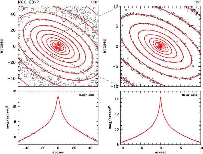
Figure 1: Upper panels: $I$-band isophotes of NGC 3377 (solid line, step of 0.5 mag/$\mathrm{arcsec}^{2}$) and, superimposed, of the axisymmetric MGE model convolved with the appropriate PSF (heavy line). Left: wide-field image (OHP, courtesy of R. Michard), right: HST/WFPC2 image. North is $20\degr$ (anti-clockwise) from the $y<0$-axis, and east is to the right. Lower panels: cut along the major axis.

For the high spatial resolution photometric data (see Fig. 1, right panel), we use $I$-band (F814W) HST/WFPC2 images, retrieved through the ST/ECF archives (PI Faber, ID 5512). The 5 individual exposures ($2\times 80$ s and $3\times 350$ s) were reduced in the standard way, and normalized in flux (in $L_{\sun}$/pc²) using the most recent PHOTFLAM conversion factors. The exposures were combined (with cosmics removal) after verifying they were properly centered.

The comparison between the two ground- and space-based flux calibrated exposures shows an offset of $\sim 0.1$ mag, mostly due to the difference in the zero points. We decided to use the HST/WFPC2 F814W image as a reference and renormalized the OHP image accordingly. The agreement between the two exposures is then excellent.

2.2 The MGE surface brightness model

We have used the Multi-Gaussian Expansion (MGE) method to model the surface brightness distribution for NGC 3377 using the photometric data described above. The routine provides an analytical model of the observed luminosity distribution, taking into account the convolution effect of the point spread function (PSF). The method assumes that both the PSF and the unconvolved surface brightness distribution of the galaxy can be described by a sum of two-dimensional Gaussians, whose best-fitting parameters are determined using an iterative approach.

Each two-dimensional Gaussian $G^{\prime}_{j}$ is described by its maximum intensity $I^{\prime}_{j}$, its dispersion $\sigma^{\prime}_{j}$ along its major axis, its flattening $q^{\prime}_{j}$, its center given by its coordinates $X^{\prime}_{j},Y^{\prime}_{j}$, and its position angle PA_j. In the general case, all components are free to have different PA and centers, an $N$-Gaussian model thus depending on $6N$ free parameters.

The MGE method has several advantages:

• the proper account of the individual PSFs allows the simultaneous use of complementary datasets with different spatial resolution (space- and ground-based observations);

• its flexibility makes it well suited for complex, multi-component galaxies such as NGC 3377, which exhibits both diskyness and boxyness (e.g. Peletier et al. 1990; Scorza & Bender 1995);

• the fitting procedure allows linear and non-linear constraints on the parameters. In the present case, since we require the deprojected model to be axisymmetric, we force the two-dimensional model to be bi-symmetric by imposing components to share the same PA and center, resulting in 3 free parameters per Gaussian.

The PSF of the OHP exposure was approximated with an MGE fit (two concentric circular Gaussians) of the extracted image of a star located several arc-minutes from the galaxy, where its background is negligible. Using this model PSF, the large-scale surface brightness distribution of NGC 3377 is well described by a sum of 6 Gaussians. Since the nuclear regions are strongly affected by seeing ($\sim 2\aas@@fstack{\prime\prime}1$ FWHM), we only keep the three outer components of this model (with $14\aas@@fstack{\prime\prime}5\leq\sigma^{\prime}_{j}\leq 72\aas@@fstack{\prime\prime}4$, Gaussians $G^{\prime}_{11}$ to $G^{\prime}_{13}$ in the final model, see Table 1), and proceed by then fitting the central part using the HST/WFPC2 exposure.

The PSF of the HST/WFPC2-PC/F814W exposure was derived with the dedicated PSF simulator TinyTim (v4.4), and consequently adjusted by a sum of three concentric circular Gaussians. The presence of dust lanes in the very central parts of NGC 3377, already noted by K+98, makes the determination of the inner Gaussians more sensitive, and hence the convergence process is slower. These dust lanes correspond to a maximal absorption of $\sim 10\%$, and the areas affected were discarded from the MGE fit. After subtraction of the properly aligned three-Gaussian ‘ground-based model’, the residual image was fitted by a sum of 10 Gaussians, describing the inner parts of NGC 3377 ($0\aas@@fstack{\prime\prime}04\leq\sigma^{\prime}_{j}\leq 6\aas@@fstack{\prime\prime}04$, Gaussians $G^{\prime}_{1}$ to $G^{\prime}_{10}$ in the final model, see Table 1). Gaussians $G^{\prime}_{5}$ and $G^{\prime}_{8}$ are significantly flatter than the others, betraying the presence of a disk.

Table 1: Parameters of the MGE deconvolved $I$-band surface brightness model of NGC 3377. $I^{\prime}_{j}$, $\sigma^{\prime}_{j}$ and $q^{\prime}_{j}$ are the intensity, the dispersion along its major axis and the flattening, of the $j$-th two-dimensional Gaussian respectively (the flattest component is indicated in italics). All the Gaussians share the same center and orientation. $I_{j}$ is the intensity of the three-dimensional Gaussian resulting from the deprojection of the corresponding two-dimensional Gaussian, assuming oblate geometry and an inclination of $i=90\degr$ (see text).

Origin	Index	$I^{\prime}_{j}$	$\sigma^{\prime}_{j}$	$q^{\prime}_{j}$	$I_{j}$
		[$L_{\sun}$/pc2]	[″]		[$L_{\sun}$/pc2/″]
HST	1	536128.0	0.037	0.833	5833935.5
	2	281535.8	0.105	0.753	1068021.9
	3	107724.4	0.248	0.520	173261.0
	4	53251.8	0.391	0.712	54347.3
	5	12739.8	0.838	0.239	6066.5
	6	30979.7	0.893	0.469	13838.3
	7	9990.8	1.994	0.495	1998.9
	8	2526.7	3.598	0.232	280.2
	9	2556.4	3.791	0.574	269.0
	10	2337.2	5.989	0.479	155.7
OHP	11	1157.1	14.456	0.475	31.9
	12	376.9	30.047	0.541	5.0
	13	82.5	72.378	0.743	0.4

The final MGE model of NGC 3377 consists of the resulting set of 13 Gaussians (see Table 1). Fig. 1 displays the contour maps of the $I$-band images with superimposed contours of the appropriately convolved MGE model, as well as cuts along the major axis. The resulting fit to the observed photometry is excellent. There is no sign of departures from axisymmetry in the central regions, and the PA of the major axis is constant with radius (e.g. Peletier et al. 1990). The total luminosity of the MGE model is $L_{I}=1.1\,10^{10}$ $L_{\sun}$, yielding $M_{I}=-21.0$. Taking a total $B-I=1.85$ (Idiart et al. 2002), we get $M_{B}=-19.15$, in good agreement with the value of $M_{B}=-19.2$ available in the LEDA database (Paturel et al. 1989).

2.3 Deprojection

The MGE modeling allows the spatial luminosity density to be analytically derived from the surface brightness model, assuming an inclination angle $i$, and that the luminosity density associated with each individual three-dimensional Gaussian is stratified on concentric ellipsoids. Each two-dimensional Gaussian $j$ then uniquely deprojects into a three-dimensional Gaussian, whose parameters $I_{j}$, $\sigma_{j}$ and $q_{j}$ can be derived from $I^{\prime}_{j}$, $\sigma^{\prime}_{j}$, $q^{\prime}_{j}$ and $i$ following relations provided in Monnet et al. (1992). The associated gravitational potential $\Phi$ can be derived easily assuming a given (constant) mass-to-light ratio $\Upsilon_{I}$ (see Emsellem et al. 1994a, for details).

The inclination $i$ of the best-fitting MGE model (see Table 1) is (formally) constrained by that of the flattest two-dimensional Gaussian to be $90\degr\geq i\geq 76.6\degr=\arccos{(\min\{q^{\prime}_{j}\}=0.232)}$. This constraint should however be treated with some caution since it is model dependent. However, no good MGE fit could be found with the additional requirement $\min\{q^{\prime}_{j}\}\geq 0.35$. This sets a robust minimum inclination of $i_{\min}\simeq 70\degr$. In the following, we will only consider the edge-on model, i.e., $i=90\degr$, since the inclination hypothesis is likely not to be the most restrictive one (see discussion in Sect. 5).

3 Kinematical data

In this Sect., we summarize the stellar kinematic measurements obtained with the integral-field spectrographs OASIS and SAURON.

3.1 OASIS observations

NGC 3377 was observed on April 1 and 2 1998 with OASIS mounted on the adaptive optics (AO) bonnette PUEO of the Canada-France-Hawaii Telescope (see Bacon et al. 1998, 2001b, for a full description of OASIS). In order to take advantage of the better performance of adaptive optics in the red, we used the MR3 configuration covering the $\@element{\mathrm{Ca}}$ triplet ($\sim 8500$ Å) region. We selected a spatial sampling of 0$\aas@@fstack{\prime\prime}$16 per hexagonal-shape lens, which provides a FoV of $6\aas@@fstack{\prime\prime}2\times 5\aas@@fstack{\prime\prime}0$. The instrumental setup is given in Table 2.

Table 2: Instrumental setup for the OASIS observations.

PUEO
Loop mode	automatic
Loop gain	80
Beam splitter	I
OASIS
Spatial sampling	0$\aas@@fstack{\prime\prime}$16
Field-of-view	$6\aas@@fstack{\prime\prime}2\times 5\aas@@fstack{\prime\prime}0$
Number of spectra	1123
Spectral sampling	2.23 Å pixel-1
Spectral resolution ($\sigma$)	70 $\mathrm{km\,s^{-1}}$
Wavelength range	8351–9147 Å

Seven 30 mn exposures centered on the nucleus (but slightly dithered to avoid systematics) were acquired, the AO being locked on the central cusp of the galaxy. The atmospheric conditions were photometric, and observations were carried out at low airmass ($<1.16$). Natural seeing conditions were mediocre with FWHM between 1″ and 1$\aas@@fstack{\prime\prime}$5, providing an AO corrected PSF with FWHM $\sim 0\aas@@fstack{\prime\prime}6$ (see Sect. 3.3.2). Neon arc lamp exposures were obtained before and after each object integration. Other configurations exposures (bias, dome flat-field, micro-pupil) were usually acquired at the beginning or the end of the nights. Twilight sky exposures were obtained at dawn or sunrise.

3.2 SAURON observations

NGC 3377 was observed on February 17 1999 with SAURON during its first scientific run on the William Herschel Telescope (Bacon et al. 2001a). The instrumental setup is summarized in Table 3. Four centered but slightly dithered 30 mn exposures were acquired, providing a total FoV of $32\arcsec\times 43\arcsec$ with an original sampling of 0$\aas@@fstack{\prime\prime}$94. The spectral coverage of SAURON includes the $\@element{\mathrm{Mg}}$ absorption triplet as well as $\@element{\mathrm{Fe}}$ and $\@element{\mathrm{Ca}}$ absorption lines, and the [O iii] and $\@element{\mathrm{H}}$$\beta$ emission lines when present.

Table 3: Instrumental setup for the SAURON observations.

SAURON
Spatial sampling	0$\aas@@fstack{\prime\prime}$94
Field-of-view	$33\arcsec\times 41\arcsec$
Number of spectra	1431
Spectral sampling	1.1 Å pixel-1
Spectral resolution ($\sigma$)	108 $\mathrm{km\,s^{-1}}$
Wavelength range	4820–5340 Å

3.3 IFS data reduction

3.3.1 Spectra extraction and calibration

The integral-field spectroscopic data were reduced according to the usual procedure described in Bacon et al. (2001b) for OASIS and Bacon et al. (2001a) for SAURON. The standard reduction procedures include CCD preprocessing, optimal extraction of the spectra, wavelength calibration, spectro-spatial flat-fielding and cosmic-ray removal.

Given the small FoV of OASIS and the high surface brightness of the nucleus of NGC 3377 ($\mu_{V}=17.7$ at 3$\aas@@fstack{\prime\prime}$3), no sky subtraction was required for this instrument. Furthermore, no flux calibration was performed for OASIS, since this is not required for measurement of the stellar kinematics.

On the SAURON exposures, after spectral resolution rectification to a common value of 1.91 Å $\sim 108$ $\mathrm{km\,s^{-1}}$(see Bacon et al. 2001a, for details), the night-sky spectrum was estimated from the dedicated sky lenslets and subtracted from the object spectra.

3.3.2 Spatial PSF estimates and datacubes merging

The knowledge of the spatial PSF is of particular importance in the modeling process, as we aim at using datasets with very different spatial resolutions. The spatial PSFs presented below have been estimated from the comparison between the images reconstructed from our IFS data and higher resolution reference frames (see details of the method in Bacon et al. 2001b). Once the individual frames were properly aligned and renormalized, the merging of multiple exposures was carried out according to the prescriptions detailed in Bacon et al. (2001a). Note that the data reduction software simultaneously provides the variance along each spectrum, which will used to estimate the local signal-to-noise in the datacube.

OASIS.

The PSF of the individual OASIS exposures is well approximated by a sum of two concentric circular Gaussians, and we estimated it by comparison with the HST/WFPC2 F814W image described in Sect. 2.1. We ranked the 7 OASIS PSFs, labeled from i to vii, according to their FWHM (see Fig. 2): 0$\aas@@fstack{\prime\prime}$56 for exposure v, $\sim 0\aas@@fstack{\prime\prime}62$ for exposures i,iii,iv and vi, and $\sim 0\aas@@fstack{\prime\prime}73$ for exposures ii and vii.

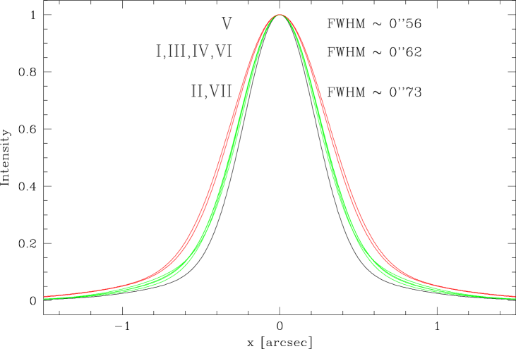
Figure 2: Fitted PSF of the 7 OASIS individual exposures. The PSFs have been approximated by a sum of 2 concentric circular Gaussians (see text). The individual PSFs can be sorted in 3 categories, with a mean FWHM of 0$\aas@@fstack{\prime\prime}$56, 0$\aas@@fstack{\prime\prime}$62 and 0$\aas@@fstack{\prime\prime}$73 respectively.

Single exposures have a signal-to-noise ratio $S/N$ which is insufficient for individual use in deriving the stellar kinematics. We have therefore constructed two merged datacubes using two different sets of exposures (trading-off between $S/N$ and resolution):

Datacube ‘A’:

includes all the individual exposures except cubes ii and vii, in order to optimize the spatial resolution;

Datacube ‘B’:

includes all seven individual exposures, in order to maximize $S/N$.

We approximate the PSF of each merged datacube by a sum of three Gaussians (see Table 4 and Fig. 3). It appears that there is not much difference in terms of effective spatial resolution between cubes ‘A’ and ‘B’, while the global $S/N$ of datacube ‘B’ is slightly higher. Hence we consider only cube ‘B’, which consists of 637 spectra with a final sampling of 0$\aas@@fstack{\prime\prime}$25.

Table 4: PSF parameters of the OASIS and SAURON merged exposures.

ID	FWHM	$\sigma_{1}$	$\sigma_{2}$	$I_{2}/I_{1}$	$\sigma_{3}$	$I_{3}/I_{1}$
OASIS/A	0$\aas@@fstack{\prime\prime}$61	0$\aas@@fstack{\prime\prime}$22	0$\aas@@fstack{\prime\prime}$45	0.33	1$\aas@@fstack{\prime\prime}$11	0.02
OASIS/B	0$\aas@@fstack{\prime\prime}$62	0$\aas@@fstack{\prime\prime}$21	0$\aas@@fstack{\prime\prime}$42	0.49	0$\aas@@fstack{\prime\prime}$96	0.04
SAURON	2$\aas@@fstack{\prime\prime}$15	0$\aas@@fstack{\prime\prime}$83	1$\aas@@fstack{\prime\prime}$80	0.20

Figure 3: Effective PSF for the OASIS (left) and SAURON (right) merged datacubes of NGC 3377. As described in the text, the OASIS PSF is highly non-Gaussian and is properly described by a sum of three Gaussians (dotted lines); the spatial resolution is estimated to be 0$\aas@@fstack{\prime\prime}$62 FWHM. The SAURON PSF is described by a double Gaussian of 2$\aas@@fstack{\prime\prime}$1 FWHM.

SAURON.

All four individual SAURON exposures have similar spatial resolution, with a FWHM ranging from 2$\aas@@fstack{\prime\prime}$0 to 2$\aas@@fstack{\prime\prime}$5 (estimated from direct images obtained before and after the SAURON observations). All of them were therefore merged in a cube of 2957 spectra over-sampled at 0$\aas@@fstack{\prime\prime}$68 to allow a proper analysis of the spatial PSF.

We approximate the spatial PSF of the SAURON merged datacube by a sum of two Gaussians and estimated their parameters by comparison with the HST/WFPC2 F555W images obtained and reduced as described in Sect. 2.1 (see Table 4 and Fig. 3). The SAURON PSF is significantly non-gaussian: the two-Gaussian approximation has a global FWHM of 2$\aas@@fstack{\prime\prime}$15, while the best fit with a single Gaussian has a FWHM of 2$\aas@@fstack{\prime\prime}$62.

In order to reduce significantly the amount of data to handle during the modeling, while retaining all the initial information, the four individual SAURON data-cubes were then merged again in a final cube of 1534 spectra sampled at 0$\aas@@fstack{\prime\prime}$94, corresponding to a strict Nyquist sampling of the spatial PSF.

3.3.3 Spatial binning

In order to increase the $S/N$, and reduce the number of independent apertures for the dynamical modeling, we applied an adaptive quadtree spatial binning to the SAURON datacube (see Appendix A). We did not apply this technique to the OASIS datacube, as we wished to retain the highest spatial resolution available. The SAURON binned datacube finally includes 475 independent spectra (see Fig. 14).

3.4 Stellar kinematics

We obtained reference stellar templates from dedicated exposures of HD 132737 for OASIS, and HD 85990 for SAURON, both of spectral type K0III. The stellar spectra were optimally summed over a spatial aperture of $R=2\arcsec$ to maximize the $S/N$ ($\sim 1300$ for OASIS and $\sim 500$ for SAURON). The resulting individual stellar spectra, as well as the final OASIS and SAURON NGC 3377 datacubes, were then continuum divided and rebinned in $\ln\lambda$. We used our own version of the Fourier Correlation Quotient (FCQ) method (Bender 1990; Bender et al. 1994) to derive the non-parametric LOSVD at every point of the final datacubes. When needed, the LOSVDs were parametrized using a simple Gaussian and complemented using 3rd and 4th order Gauss-Hermite moments $h_{3}$ and $h_{4}$ (van der Marel & Franx 1993; Gerhard 1993). We checked that similar results were obtained with an updated version of the cross-correlation method (Statler 1995), and that these did not significantly depend on the details of the continuum subtraction procedure.

Fig. 4 and 5 present the kinematic maps (mean velocity $V$, velocity dispersion $\sigma$, Gauss-Hermite moments $h_{3}$ and $h_{4}$) for OASIS and SAURON respectively, in the setup used for the dynamical modeling (see Sect. 4).

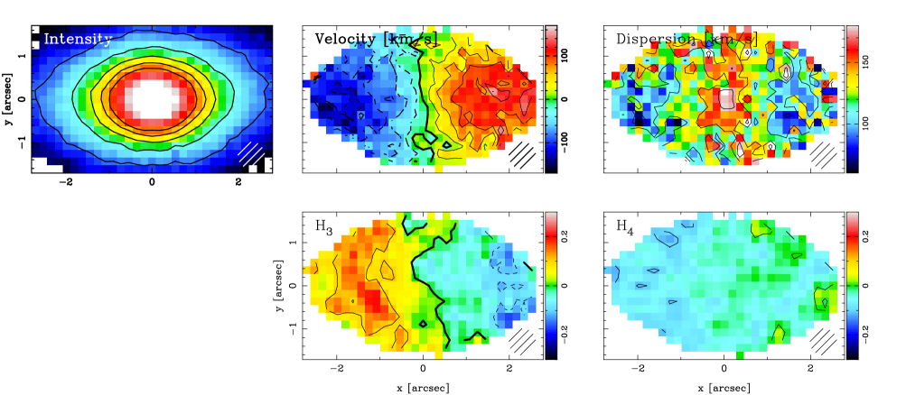
Figure 4: OASIS stellar kinematical maps (filtered: $S/N_{\min}=40$). In each panel, the hatched disk corresponds to the size of the seeing disk of 0$\aas@@fstack{\prime\prime}$62 FWHM.

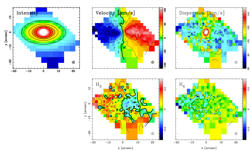
Figure 5: SAURON stellar kinematical maps. In each panel, the hatched disk corresponds to the size of the seeing disk of 2$\aas@@fstack{\prime\prime}$1 FWHM.

Estimates of the errors on each velocity bin of the non-parametric LOSVDs are obtained by means of a Monte-Carlo approach (see Copin 2000): for each galaxy position, a noise-free galaxy spectrum is built by convolving the template spectrum with the corresponding parametrized LOSVD. We then add noise realizations (consistent with the derived noise spectra of the datacube), and extract the LOSVD via FCQ. The error is defined as the variance of the distribution at each velocity bin after 100 realizations. If needed, errors on the measured kinematical parameters are derived from the same procedure, which produces reasonably realistic error-bars (see e.g. Fig. 6 and 7; see also de Bruyne et al. 2003).

3.4.1 Comparisons with different datasets

We checked that the OASIS and SAURON datasets were consistent with each other, not only regarding their surface brightness distribution from which the PSFs were estimated, but also by comparing $V$ and $\sigma$ maps. The OASIS FoV is too small to allow proper convolution to the SAURON resolution. We therefore built a simple analytical model which approximates the ‘intrinsic’ $V$ and $\sigma$ fields, and used the MGE photometry model to convolve this model with the adequate PSFs. The agreement between the kinematics obtained with OASIS and SAURON is excellent, as shown in Fig. 6.

Figure 6: Comparison along the major axis between the OASIS (open circles) and SAURON (closed circles) datasets (upper panel: mean velocity, lower panel: velocity dispersion), and the simple analytic models convolved to the proper OASIS (dashed line) and SAURON (solid line) resolutions.

We also compared the OASIS and SAURON stellar kinematics with measurements based on long-slit data published by Bender et al. (1994, Calar Alto, slit width of 2$\aas@@fstack{\prime\prime}$1, spectral resolution of 46 $\mathrm{km\,s^{-1}}$, hereafter BSG94), K+98 (spectrograph SIS/CFHT, slit width $\sim 0\aas@@fstack{\prime\prime}3$–0$\aas@@fstack{\prime\prime}$5, spectral resolution $\sim 40$–60 $\mathrm{km\,s^{-1}}$) and Simien & Prugniel (2002, spectrograph CARELEC/OHP, slit width of 1$\aas@@fstack{\prime\prime}$5, spectral resolution of 25 $\mathrm{km\,s^{-1}}$, hereafter SP02). A proper comparison between these different datasets is difficult because of the very different spatial resolutions and instrumental setups. We therefore restricted these comparisons to the datasets which share similar spatial resolutions, i.e., OASIS with K+98 and SAURON with BSG94 and SP02. The IFS data were thus binned according to the characteristics of the long-slit data and compared as shown in Fig. 7: the datasets are in good agreement, particularly considering the difficulty mentioned above. The (marginal) 0$\aas@@fstack{\prime\prime}$15-offset reported by K+98 in the mean velocity profile is not seen in our OASIS data.

We chose not to use the FOS observations of the nucleus of NGC 3377 (G+03, square aperture of 0$\aas@@fstack{\prime\prime}$21, spectral resolution of $\sim 100$ $\mathrm{km\,s^{-1}}$, no aperture illumination corrections applied) for three reasons: (a) the lack of extensive spatial information makes the comparison with such high-spatial resolution data hazardous, (b) the proper determination of aperture positioning is known to be a critical procedure (van der Marel et al. 1997), potentially leading to critical consequences for the dynamical modeling, (c) by excluding these measurements, our dynamical models are fully independant to the ones developed by G+03.

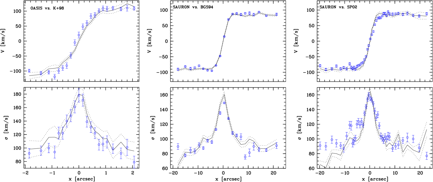
Figure 7: Comparison between the long-slit stellar kinematics from literature (points) and the equivalent IFS kinematics (lines) for the mean velocities (top) and velocity dispersions (bottom): OASIS vs. K+98 (left), SAURON vs. BSG94 (middle) and SAURON vs. SP02 (right). The dotted lines give the 1-$\sigma$ error on the IFS parameters, as estimated from Monte-Carlo simulations.

3.4.2 First results from the SAURON and OASIS maps

As mentioned earlier, the OASIS and SAURON kinematics presented in Fig. 4 and 5 respectively are fully coherent and in excellent agreement with the long-slit datasets previously published, up to the highest spatial resolutions. The steep velocity gradient, unresolved at the SAURON resolution, reaches a maximum of $\sim 110$ $\mathrm{km\,s^{-1}}$ at $r\approx 1\aas@@fstack{\prime\prime}5$, and then decreases to a plateau of $\sim 90$ $\mathrm{km\,s^{-1}}$. The velocity dispersion peak is barely spatially resolved in the OASIS observations, and reaches $\sim 170$ $\mathrm{km\,s^{-1}}$. The $h_{3}$ coefficient is anti-correlated with the mean velocity as expected from the superposition of a bright dynamically cold component on a hotter spheroid.

Integral-field spectroscopy enables us to analyse the ‘morphology’ of the kinematics, something not possible using long-slit spectra. Both OASIS and SAURON mean velocity fields reveal a twist of the zero velocity curve of $\sim 10^{\circ}$ with respect to the photometric minor-axis up to $r\approx 10\arcsec$, while the photometry does not show any variation of position angle (Peletier et al. 1990). As a consequence, the velocities along the minor-axis are not null, a fact not reported so far, and which is clearly visible with an amplitude of $\sim 7$ $\mathrm{km\,s^{-1}}$ for OASIS and $\sim 12$ $\mathrm{km\,s^{-1}}$ for SAURON.

The SAURON velocity dispersion-map also presents interesting morphological features: while the $\sigma$-peak is elongated along the photometric minor-axis – consistent with the diskyness of the light distribution –, it displays a twist of about $10^{\circ}$ in the direction opposite to the kinematic misalignment. These modest but significant departures from axisymmetry are probable signatures of a triaxial intrinsic shape. This is also apparent in the ionized gas distribution and motions, which exhibit a noticeable spiral-like morphology and strong departures from circular motions (Bacon et al. 2001a). These issues will be discussed in more detail in a forthcoming paper .

4 Dynamical models

4.1 Schwarzschild models

We construct dynamical models based on the orbit superposition technique of Schwarzschild (1979, 1982). Similar orbit-based models were constructed to measure the masses of central BHs (van der Marel et al. 1998; Cretton & van den Bosch 1999; Verolme et al. 2002; Cappellari et al. 2002; Gebhardt et al. 2003), and dark halo parameters (Rix et al. 1997; Gerhard et al. 1998; Saglia et al. 2000; Kronawitter et al. 2000). Our implementation is described in detail in Cretton et al. (1999, hereafter C99). We summarize it briefly here.

We sample the stellar orbits using a grid in integral space, which includes: the energy $E$, the vertical component of the angular momentum $L_{z}$ and an effective third integral $I_{3}$. We use 20 values of $E=1/2\;R_{c}\;\partial\Phi/\partial R+\Phi(R_{c},0)$, sampled through the radius of the circular orbit $R_{c}$. We take a logarithmic sampling of $R_{c}$ in $[0\aas@@fstack{\prime\prime}01,300\aas@@fstack{\prime\prime}0]$, since more than 99% of the total mass of our MGE model lies inside this range. 14 values of $L_{z}$ per $E$ in $[-L_{z,\max},+L_{z,\max}]$ and 7 values of $I_{3}$ per ($E,L_{z}$) were adopted (see C99).

The orbit library is constructed by numerical integration of each trajectory for an adopted amount of time (200 periods of the circular orbit at that $E$) using a Runge-Kutta scheme. During integration, we store the fractional time spent by each orbit in a Cartesian ‘data-cube’ $(x^{\prime},y^{\prime},v_{\mathrm{los}})$, where $(x^{\prime},y^{\prime})$ are the projected coordinates on the sky and $v_{\mathrm{los}}$, the line-of-sight velocity. We use an $E$-dithering scheme (see C99) to make each orbit smoother in phase space. The data-cube of each individual orbit is further convolved with the PSF and eventually yields the orbital LOSVD $\mathcal{L}_{(x^{\prime},y^{\prime})}(v_{\mathrm{los}})$ at each position $(x^{\prime},y^{\prime})$ on the sky.

In C99, we adopted a parametrized form for the (orbital and observed) LOSVDs using the Gauss-Hermite series expansion. However, as emphasized in Cretton & van den Bosch (1999), some problems may arise in the modeling of dynamically ‘cold’ systems (i.e., with a high $V/\sigma$), where the use of the linear expansion can lead to spurious counter-rotation. To avoid this potential shortcoming, we choose to constrain the dynamical models using directly the full non-parametrized LOSVDs. As a consequence, the maps presented in Fig. 4 and 5 are shown for illustration purposes, but were not used in the modeling technique.

Orbital occupation times are also stored in logarithmic polar grids in the meridional plane and in the $(x^{\prime},y^{\prime})$ plane, to make sure the final orbit model reproduces the MGE mass model. The mass on each orbit is computed with the NNLS algorithm (Lawson & Hanson 1974), such that the non-negative superposition of all orbital LOSVDs aims at reproducing the observed LOSVDs within the errors. In addition, the model has to fit the intrinsic and projected MGE mass profiles. Smoothness in integral space can be enforced through a regularization technique (see C99). Models with different values of BH mass $M_{\bullet}$ and mass-to-light ratio $\Upsilon_{I}$ are constructed and compared to the data. As mentioned in Sect. 2.3, the mass-to-light ratio $\Upsilon_{I}$ is assumed to be constant over the whole extent of the galaxy. The quality of the fit is assessed through a $\chi^{2}$-scheme and we use the $\delta\chi^{2}=\chi^{2}-\chi^{2}_{\min}$ statistic to assign confidence values to the iso-$\chi^{2}$ contours (e.g. Cretton et al. 2000; Gebhardt et al. 1996).

The main differences with respect to models previously published are (a) the use of the full non-parametrized LOSVDs (but see Gebhardt et al. 2000; Bower et al. 2001; Gebhardt et al. 2003), (b) the two-dimensional coverage of the data (but see Cappellari et al. 2002; Verolme et al. 2002). Most previous studies made use of long-slit 1D-data at a few position angles (e.g. van der Marel et al. 1998), but the advance of IFU spectrographs (e.g. OASIS/CFHT, SAURON/WHT, FLAMES and VIMOS at the Very Large Telescope, etc.) will deliver two-dimensional data for many objects. A more detailed study of the effect of using such two-dimensional constraints will be presented in a companion paper (Cretton & Emsellem, in preparation).

4.2 SAURON constraints with original errors

We compute a grid of orbit libraries with $M_{\bullet}$ ranging from $0.0$ to $1.82\,10^{8}$ $M_{\sun}$ and $\Upsilon_{I}$ between $2.2$ and $2.6$. First, we constrain these models only with the SAURON dataset and $\delta\chi^{2}$-contours are showed in Fig. 8 (left panel). At 99.7% confidence level, the allowed $M_{\bullet}$ is smaller than $\sim 2\,10^{7}$ $M_{\sun}$. This appears to be surprisingly small, given the low spatial resolution ($\sim 2\aas@@fstack{\prime\prime}1$ FWHM) of the SAURON dataset. Indeed, in the case of NGC 3377 with a characteristic central velocity dispersion of $\sigma\sim 135$ km/s and an assumed distance of $D=9.9$ Mpc, this spatial resolution corresponds roughly to the radius of influence of a $1.6\,10^{8}$ $M_{\sun}$ BH (de Zeeuw 2001).

Figure 8: Left panel: $\delta\chi^{2}$-contours based on SAURON data and original (statistic) errors. Each dot represents a model run. The thick contour corresponds to the 99.7% confidence level. Right panel: Same as left panel, but with a larger orbit library ($\times 8$). Differences between the two plots are small.

In order to check that the tightness of the $\delta\chi^{2}$-contours is not an artifact of our choice of technical implementation, we have constructed several orbit libraries, changing one parameter of the library at a time: (a) the length of each orbit integration has been increased up to 1000 radial periods, (b) the $E$-sampling of the library has been refined, (c) the individual orbital time-steps have been decreased, and (d) the size of the orbit library has been increased by eight-fold, $(N_{E},N_{L_{z}},N_{I_{3}})=(40,28,14)$ instead of $(20,14,7)$. For the latter model, the resulting $\delta\chi^{2}$-contours are shown in the right panel of Fig. 8: although the orbit library was expanded by a factor of 8, the upper limit for $M_{\bullet}$ is still surprisingly small. In fact, none of the above modifications affected the tightness of the $\delta\chi^{2}$-contours in a significant way. We conclude that this peculiar result is not related to specific technical details of our modeling method.

4.3 Departures from axisymmetry

To test further the origin of the tightness of the $\delta\chi^{2}$-contours for the SAURON dataset, we constructed fake constraints drawn from an isotropic distribution function $f(E,L_{z})$, using the Hunter & Qian (1993) method (hereafter HQ). The even part of such a DF is uniquely specified by the mass profile and we choose the odd part such as to mimic the true observed SAURON kinematics. A $10^{8}$ $M_{\sun}$ BH has been included into the HQ model. HQ-LOSVDs are then computed in the SAURON setup: they are convolved with the SAURON PSF and binned into the SAURON spatial elements. This artificial dataset looks very similar to the SAURON data, but a dynamical fit gives very different $\delta\chi^{2}$-contours, allowing BH masses up to $1.5\,10^{8}$ $M_{\sun}$ at 99.7% confidence level. For this fit, we have used ad-hoc error-bars equal to 5% of the largest LOSVD value in each pixel. In each SAURON pixel, these errors are therefore independent of $v_{\mathrm{los}}$. With such a choice of errors, we are conservative in the sense that real observed errors are (on average) three times higher and would therefore induce even wider $\delta\chi^{2}$-contours.

By construction, the HQ data correspond to a perfectly axisymmetric galaxy, and are therefore fully [anti-]bi-symmetric, i.e., $\mathcal{L}_{(x^{\prime},y^{\prime})}(v_{\mathrm{los}})=\mathcal{L}_{(-x^{\prime},y^{\prime})}(-v_{\mathrm{los}})=\mathcal{L}_{(x^{\prime},-y^{\prime})}(v_{\mathrm{los}})$. In that sense, as mentioned earlier, the observed SAURON data show noticeable departure from axisymmetry, and the fit of an axisymmetric model to them will significantly increase both $\chi^{2}$ and $\delta\chi^{2}$.

If one still wishes to model non-axisymmetric data with an axisymmetric code, there are two possibilities: (a) symmetrize the data, while keeping the statistical error-bars, (b) increase the error-bars to encompass the systematic errors (if any) between the 4 quadrants. While the first solution was adopted by G+03, we chose the second option to keep as much as possible the original spatial extent of the integral-field data. For the central parts of the SAURON dataset (roughly $|x^{\prime}|\leq 12\arcsec$ and $|y^{\prime}|\leq 6\arcsec$), for which measures from the 4 quadrants are accessible, the error-bar including systematics is taken as $\sigma_{\mathrm{+syst}}^{2}=\langle\sigma^{2}\rangle_{4}+\mathrm{Var_{4}(\sigma^{2})}$, where $\mathrm{Var_{4}}$ is the variance between the four LOSVDs of the four quadrants and $\langle\sigma^{2}\rangle_{4}$ is the mean statistical error-bar of the four LOSVDs. In the outer parts, the spatial binning and the incomplete coverage of the SAURON data make the computation more difficult: we estimate the systematic errors by taking the immediate neighbor spatial element (after folding all 4 quadrants on one) if there is no symmetric correspondent in the other quadrants.

As expected, we obtain the same contours using either original or symmetrized SAURON data when the error-bars including systematics are used.

4.4 IFU constraints with errors including systematics

SAURON dataset.

Fig. 9 (left panel) shows the $\delta\chi^{2}$-contours using only the SAURON data with the errors including systematics. While the constraint on the upper limit of $M_{\bullet}$ is noticeably relaxed (the largest allowed BH mass is now $10^{8}$ $M_{\sun}$), $\Upsilon_{I}$ is strongly restricted to the range $[2.05,2.45]$ (99.7% confidence level), due to the large SAURON FoV.

Figure 9: $\delta\chi^{2}$-contours with errors including systematics. Left panel: SAURON dataset only, middle panel: OASIS dataset only, right panel: both SAURON and OASIS datasets.

OASIS dataset.

The OASIS data also show signs of non-axisymmetry (see Fig. 4), so we applied the procedure described in the previous Sect. to compute systematic error-bars. Fig. 9 (middle panel) shows the $\delta\chi^{2}$-contours constrained only with the OASIS data (restricted to the central $4\arcsec\times 2\arcsec$ part, see Fig. 10). The 99.7% confidence level is much larger than in the SAURON case: as could be expected (e.g. G+03) $\Upsilon_{I}$ is very weakly constrained due to the small extension of the data. However, a model without BH is excluded by the OASIS data at a 99.7% confidence level.

Combined datasets.

Fig. 9 (right panel) shows the results of a combined fit on both datasets. Since this fit includes all available IFU data, it presumably provides the best estimate of the BH mass and the stellar $\Upsilon_{I}$. To improve such estimates based on a grid interpolation, we compute additional models corresponding to new values of $\Upsilon_{I}-M_{\bullet}$. The best fitting model has $M_{\bullet}=7.0\,10^{7}$ $M_{\sun}$ and $\Upsilon_{I}=2.05$ (see the best-fit maps in Fig. 10 and 11, to be compared with the observed maps in Fig. 4 and 5). The minimum and maximum BH mass allowed by these data (99.7% confidence level) are $2.5\,10^{7}$ $M_{\sun}$ and $1.25\,10^{8}$ $M_{\sun}$ respectively.

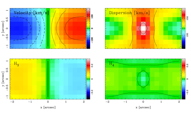
Figure 10: Best-fit stellar kinematical maps for the OASIS dataset, to be compared with Fig. 4.

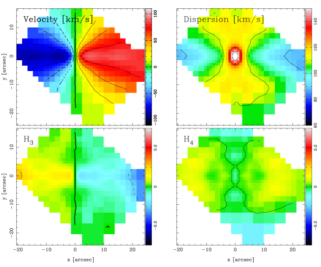
Figure 11: Same as Fig. 10 for the SAURON dataset, to be compared with Fig. 5.

4.5 Regularized models

In previous Sects., we have explored models with no requirements on the smoothness of the solution. As a result, the orbital weights are jagged and can strongly vary from one orbit to the next. One can include regularization constraints in order to obtain smoothly varying solutions (see e.g. C99). From such regularized solutions smooth functions characterizing the internal dynamical structure can be computed (see Fig. 13). But there is a much more important reason to derive regularized models. Recently, Valluri et al. (2002) have shown that (unregularized) orbit-based models do not provide reliable BH mass estimates, because the $\chi^{2}$-contours on which they are based depend strongly on the number of orbits in the library: if one increases the number of orbits, the contours get wider and the indeterminacy on the BH grows. In a forthcoming paper, we have explored this issue with component-based $f(E,L_{z})$ models and have also observed such a significant widening of the contours when the orbit library is expanded. Our tests also show that regularization may provide a way to ‘stabilize’ the $\chi^{2}$-contours, while increasing the number of orbits . Although we do not have yet a clear physical justification for the regularization scheme, we decided to apply such a procedure to construct regularized models of NGC 3377. We refer the reader to the companion paper for a discussion of these issues, outside the scope of this paper.

Fig. 12 shows the combined fit, including regularization constraints. The level of regularization has been adjusted from a comparison with the HQ models according to the prescription of C99 (their Fig. 8). The contours are then very similar to the case without regularization, and the best fitting values are almost unchanged with respect to the unregularized model with the exception of the slightly restricted maximum allowed BH mass, which is now $1.1\,10^{8}$ $M_{\sun}$. The values we adopt are thus $M_{\bullet}$ in the range 2–$11\,10^{7}$ $M_{\sun}$ (99.7% confidence level), with a best fit value of $7\,10^{7}$ $M_{\sun}$ for a mass-to-light ratio of $\Upsilon_{I}=2.1\pm 0.2$, and an assumed distance of 9.9 Mpc. Note that at the 68% confidence level, our model is well constrained with $M_{\bullet}$ between $6$ and $8\,10^{7}$ $M_{\sun}$.

Figure 12: $\delta\chi^{2}$-contours based on both SAURON and OASIS data with errors including systematics and regularization constraints.

4.6 Internal dynamical structure

To describe the internal dynamical structure of NGC 3377, we compute the velocity dispersion profiles of the best-fit orbit model: $\sigma_{r}$, $\sigma_{\theta}$ and $\sigma_{\phi}$, where $(r,\theta,\phi)$ are the usual spherical coordinates (see Fig. 13). We use the regularized models constrained on both SAURON and OASIS datasets with errors including systematics (see previous Sect.). In Fig. 13, we also plot the ratios $\sigma_{r}/\sigma_{\theta}$, and $\sigma_{r}/\sigma_{\phi}$ to better estimate the anisotropy.

The meridional plane $(R,z)$ is divided into a polar grid with seven angular sectors for $\theta\in[0,\pi/2]$ (see Sect. 4.1); the first sector is close to the symmetry axis, while the last one is near the equatorial plane. We decide to discard the sector closest to the symmetry axis (i.e., the first one), because only few orbits with very small $L_{z}$ can reach it. To reduce the noise, we average sectors two by two: #2 with #3, #4 with #5 and finally sectors #6 with #7, in the left, middle and right panels respectively (see Fig. 13).

In each panel, the vertical dashed lines indicate the extent of the kinematic data: it thus delineates the region where the models are directly constrained. Going from the symmetry axis toward the equatorial plane, the best-fit model (with $M_{\bullet}=7\,10^{7}$ $M_{\sun}$) shows an increasing radial anisotropy. It is however relatively close to isotropy, with dispersion ratios $\sigma_{r}/\sigma_{\theta}$ and $\sigma_{r}/\sigma_{\phi}$ of about 1.2. Except for the peak of $\sigma_{r}/\sigma_{\phi}$ in the central part of the equatorial plane profile, the model shows a rather constant anistropy along each (averaged) sector.

Although our mass model contains two flat Gaussian components ($G^{\prime}_{5}$ and $G^{\prime}_{8}$, see Table 1) with $q^{\prime}_{j}<0.24$, the internal structure of our best-fit model of NGC 3377 does not exhibit a strong dynamical signature of a disk like in NGC~4342 (see Fig. 13 and §7.3 of Cretton & van den Bosch 1999). Indeed, in the case of NGC 3377, these two flat components never dominate the local mass density, whereas in NGC 4342 the outer disk starts to dominate outside of 4″, inducing a radial anisotropy.

G+03 observed a ‘peak’ in $\sigma_{r}/\sigma_{\theta}$ between $r=0\aas@@fstack{\prime\prime}1$ and 1″ in the equatorial plane (see their Fig. 13). This ratio reaches 1.5 in their best-fit model, whereas we observed values below 1.2 in the same radial range. The differences are certainly due to the significantly different spatial coverage of the datasets used to constrain the models.

Figure 13: Internal dynamics of a regularized model with with $M_{\bullet}=7\,10^{7}$ $M_{\sun}$ and $\Upsilon_{I}=2.1$ for different angular sectors (see text). The first row displays the three components of the velocity dispersion ellipsoid in km/s: $\sigma_{r}$ (solid line), $\sigma_{\theta}$ (dashed line) and $\sigma_{\phi}$ (dotted line). The second and third rows show the ratios $\sigma_{r}/\sigma_{\theta}$ and $\sigma_{r}/\sigma_{\phi}$.

4.7 Comparison with previous models

The dynamics of NGC 3377, and the presence of a central massive BH, have been first studied by K+98 with isotropic models, and in greater details by G+03. The modeling technique (3$I$-Schwarzschild) and initial assumptions (axisymmetry, edge-on, constant mass-to-light ratio) used by G+03 are similar to the ones we applied on our NGC 3377 integral field data. A few important differences should be emphasized though. Firstly, G+03 constrained the spatial luminosity to be constant on homothetic ellipsoids, which may cause significant differences in the resulting dynamical model (and internal structure). However, considering that isophotes of NGC 3377 are reasonably well approximated by ellipses (with constant ellipticity), this is probably not critical in the present case. Secondly, G+03 included the FOS apertures in their list of observable constraints. As noted by G+03, the inclusion of HST measurements improves the significance of the BH detection, but does not alter significantly the upper limit of the mass estimates. The uncertainty on the actual location of the FOS apertures and its corresponding kinematics (see Sect. 3.4.1) furthermore motivated our choice of excluding this dataset.

G+03 found a BH mass of $M_{\bullet}=1.0^{+0.9}_{-0.1}\,10^{8}$ $M_{\sun}$ ($1\sigma$ range, one degree of freedom, for an assumed distance of 11.2 Mpc). This translates into a mass range for the $M_{\bullet}$ of about $8-17\,10^{7}$ $M_{\sun}$ at a distance of 9.9 Mpc. However, as explained by the authors, the lower limit on $M_{\bullet}$ is solely constrained by the 2 nuclear FOS LOSVDs: the fit on their ground-based data – stellar $V$ and $\sigma$ measurements from K+98 (see Sect. 3.4.1) – is consistent with the absence of central BH (their Fig. 7). Our best fit value of $M_{\bullet}=7\,10^{7}$ $M_{\sun}$ is just at the edge of the 95% confidence contours derived by G+03, but outside their 68% confidence mass range (see their Fig. 3).

Regarding the mass-to-light ratio, the best-fit value of $\Upsilon_{V}=2.9^{+0.1}_{-0.6}$ at $D=11.2$ Mpc found by G+03 (99.7% level) corresponds to $\Upsilon_{I}\sim\mathbf{2.16}^{+0.08}_{-0.45}$ at 9.9 Mpc (for a mean color index $(V-I)=1.14$, Goudfrooij et al. 1994, and a standard Cousins $(V-I)_{\sun}=0.685$, Bessell 1979), consistent with our best fit value of $\Upsilon_{I}=2.1$. At the 68% level, we obtain a narrow range of allowed $\Upsilon_{I}$, between 2.02 and 2.12, a significant improvement compared to the corresponding range of 1.71–2.24 found by G+03. The main reason for our better mass-to-light ratio constraint certainly lies in the spatial coverage of our kinematical datasets: G+03 only disposed of major-axis (long-slit) profiles (with the addition of the FOS apertures). As shown in Fig. 9, the SAURON dataset with its two-dimensional coverage on a relative large field strongly constrains $\Upsilon$ (assumed to be constant).

Using the combined SAURON and OASIS datasets, we therefore significantly improve the constraints on both $M_{\bullet}$ and $\Upsilon$. While our ground-based data spatial resolution is coarser than the HST spatial-grade resolution, we believe, given our aforementioned concerns regarding the uncertainties on critical kinematic measurements derived from FOS apertures, that our BH mass estimate is overall more robust than G+03’s. In addition, we think that our mass-to-light ratio estimate is better because of the extended spatial coverage of our kinematical datasets.

5 Discussion

The kinematic data used to constrain the dynamical modeling presented in this paper were exclusively obtained from two integral-field spectroscopic observations of NGC 3377. The full spatial coverage allows a proper estimate of the respective PSF (see Sect. 3.3.2), and a detailed comparison of the datasets, insuring their internal consistency (see Sect. 3.4.1). Furthermore, the spatial complementarity of the datasets – SAURON covers a relatively large FoV while OASIS probes the central parts with sharper spatial resolution – plays a key role in the modeling process (see Sect. 4.4).

Our implementation of the Schwarzschild technique has been extended to support 2D-coverage and non-parametrized LOSVD fit, and includes regularization constraints minimizing the ‘contours widening’ effect described by Valluri et al. (2002). However, our models still depend on three major assumptions, namely a given inclination, axisymmetry, and a constant mass-to-light ratio.

Inclination.

The galaxy NGC 3377 is known not to be strictly edge-on, as strongly hinted from the ionized gas distribution (Bacon et al. 2001a, if the gas is confined in the equatorial plane). However, NGC 3377 is certainly close to edge-on ($i\ga 70^{\circ}$, see Sect. 2.3) given its apparent flattening (E5-6). Running a full grid of dynamical models over the allowed range of inclinations (as in, e.g. Gebhardt et al. 2000; Verolme et al. 2002), might not be relevant if, as suspected, the assumption of axisymmetry is the most restrictive one.

Axisymmetry.

As already mentioned, a $\sim 10^{\circ}$ kinematic misalignment is observed both in the OASIS and SAURON datasets, in contradiction with an intrinsic axisymmetric morphology (while the photometry does not show any position angle twist). This non-axisymmetry could be due to the presence of an inner bar . While the observed non-axisymmetry weakens the results of our axisymmetric models, it is not clear whether it is critical for the global understanding of the intrinsic dynamics of this ‘nearly oblate’ galaxy (Davies et al. 1983) – contrary to more extreme cases (e.g. NGC 4365, Davies et al. 2001; Verolme et al. 2003) – and wether it prevents our $(M_{\bullet},\Upsilon)$ best-fit parameters to be taken into consideration.

Mass-to-light ratio.

We can compare the dynamical estimate of our $\Upsilon$ (obtained via Schwarzschild modeling) to the one independently inferred from observed colours and line strengths. Idiart et al. (2003) estimated the metallicity of NGC 3377 using broad-band colours, and derived a central and global $[Fe/H]$ of $+0.0$ and $-0.2$ respectively. Using Vazdekis et al. (1996) stellar population synthesis models with observed colors $B-V\sim 0.86$ and $V-I\sim 1.14$, this corresponds to a $\Upsilon_{V}$ in the (loose) range 2.7–3.7. Our best-fit model has $\Upsilon_{I}=2.1$, or $\Upsilon_{V}=3.2$, fully consistent with these estimates (but see discussion in Maraston 1998; Thomas et al. 2003). We also checked that the SAURON line strength values ($\@element{\mathrm{H}}$$\beta$, $\@element{\mathrm{Mg}}$b, $\@element{\mathrm{Fe}}$5015, $\@element{\mathrm{Fe}}$5270) observed for NGC 3377 are within the ranges predicted by the Vazdekis et al. models. This independent check is important as it links the stellar populations to the dynamical observables.

Regarding our central BH mass measurement, the only independent estimate we can provide, beside comparison to previously published dynamical models (see Sect. 4.7), is by using the $M_{\bullet}-\sigma$ relation: Merritt & Ferrarese (2001) and Tremaine et al. (2002) used stellar dispersion (central or effective) values of 131 and 145 $\mathrm{km\,s^{-1}}$ respectively, providing $M_{\bullet}=1.47(\pm 0.72)\,10^{7}$ and $M_{\bullet}\simeq 3.7(\pm 1.7)\,10^{7}$ $M_{\sun}$, respectively. The range of allowed $M_{\bullet}$ derived from our Schwarzschild models overlap with both estimates, although our best-fit value is clearly outside these two ranges.

Studying the importance of the effect of triaxiality is outside the scope of this paper and will be done in the future using generalized modelling techniques . In that respect, it is noticeable that only a two-dimensional coverage can properly trace the non-axisymmetry. This has consequences not only for the specific case of NGC 3377, the non-axisymmetry of which was ignored before, but probably for many other galaxies and related studies.

6 Conclusions

We have presented a unique set of nested integral-field spectroscopic observations of the E5-6 ‘disky/boxy’ cuspy galaxy NGC 3377, obtained with the OASIS and SAURON instruments. Both sets display regular stellar kinematics, with indications for an inner disk, coherent with the diskyness of the light distribution up to $\sim 30\arcsec$. However, the IFS observations also reveal a significant twist of the line of zero velocity of $\sim 10^{\circ}$ up to $r\approx 10\arcsec$ – with no corresponding isophotal twist – indicative of a moderately triaxial intrinsic shape or of a central bar.

Based on this complementary and intrinsically coherent dataset, we have constructed general (three-integral) axisymmetric dynamical models for this galaxy using the orbit superposition technique of Schwarzschild, non-parametrically fitting the full LOSVDs delivered by the 3D spectrographs. In order to properly take into account the observed non-axisymmetry of the kinematic maps, we have added a systematic component to the Monte-Carlo-computed statistical errors on the LOSVDs used in the fit. The best-fit model has a BH mass of $M_{\bullet}=7_{-5}^{+4}\,10^{7}$ $M_{\sun}$ and a mass-to-light ratio $\Upsilon_{I}=2.1\pm 0.2$ (99.7% confidence level) for an assumed distance of $D=9.9$ Mpc.

The use of fully coherent IFS measurements on the observation side, and of proper errors and regularization constraints on the modeling side allowed us to derive this significantly improved constraints on both $\Upsilon$ and $M_{\bullet}$. However, some assumptions used in the modeling – the most important presumably being the axisymmetry – are in noticeable contradiction with our IFS observations. Therefore, BH mass estimates for NGC 3377 based on axisymmetric models should be considered with caution.

Appendix A Adaptive quadtree two-dimensional binning

In order to increase the $S/N$ in the outer parts of the SAURON exposure, we used an adaptive spatial binning algorithm. A detailed account of binning techniques is described in Cappellari & Copin (2003).

While filtering (i.e., ‘smoothing’) spectrographic data is equally easy for long-slit and integral-field spectrographs, data binning is much trickier for two-dimensional data, due to the topological constraints (i.e., the proper tiling of the plane). Still, proper binning of two-dimensional data is necessary when we wish to compare them with theoretical or numerical models.

The first step is to estimate the flux and mean $S/N$ at each spatial element (hereafter spaxel). In the present case, each spaxel $i$ of the input cube is associated to the spectrum $S_{i}(\lambda)$, and one can compute the total flux ${\cal S}_{i}=\int S_{i}(\lambda)\,\mathrm{d}\lambda$ by integrating along the spectral dimension, as well as the mean signal-to-noise ratio $\eta_{i}=\langle S_{i}(\lambda)/\sigma_{i}(\lambda)\rangle_{\lambda}$, where $\sigma_{i}(\lambda)$ is the chromatic variance as estimated during the data-reduction process. Furthermore, the real $({\cal S}_{i},\eta_{i})$-spaxels are embedded in a $2^{n}\times 2^{n}$-grid, otherwise completed with $(0,0)$-spaxels.

The algorithm is then as follows:

Initialization.

All the spaxels of the input grid are associated in a single bin, with flux ${\cal F}_{1}=\sum_{i}{\cal S}_{i}$ and mean signal-to-noise $\zeta_{1}={\cal F}_{1}/\sum_{i}({\cal S}_{i}^{2}/\eta_{i}^{2})$. Hopefully, this 1-bin has a $S/N$ high enough to be divided further and initialize the process.

Iteration.

If $m$-bin $j$ is indeed a bin – i.e., contains at least 4 spaxels – and has high enough a $S/N$ with respect to the target $S/N$, it can be divided further into 4 subsequent $(m+1)$-bins. Since the initial grid had a power-of-two side length, all the child-bins also have a power-of-two side length.

Conclusion.

All the bins which are not completely covered by real data (in our case, 80%) or whose $S/N$ is lower than a given threshold are then discarded.

This method leads naturally to an Unbalanced Quadtree spatial binning of the original datacube (e.g. Bern & Eppstein 1995). Contrarily to the optimal binning presented in Cappellari & Copin (2003), this quadtree binning does not produce a very homogeneous $S/N$ distribution over the field. However, it provides simple shapes – squares – for the final bins, and therefore simplify the comparison with models.

For the specific case of the SAURON NGC 3377 data, we have used a target $S/N$ of 50 and a minimum $S/N$ of 30. This resulted into 475 independent binned spectra as shown in Fig. 14.

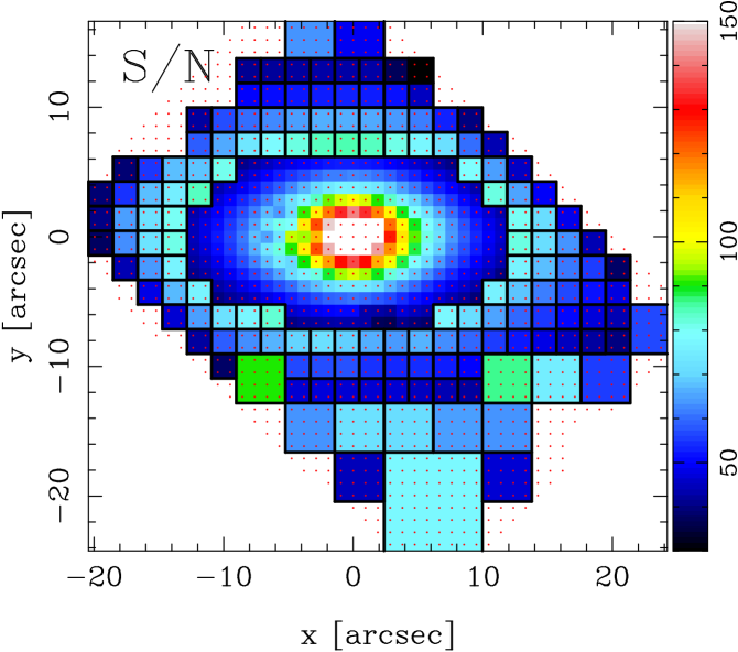
Figure 14: Unbalanced Quadtree spatial binning of the SAURON datacube resulting from the method described in the text. The dots show the location of the initial SAURON spaxels, and the squares display the boundaries of the multi-spaxel bins.