Q-LET — Quick Lensing Estimation Tool
An application to SN2003es

Abstract

Q-LET is a FORTRAN 77 code that enables a quick estimate of the gravitational lensing effects on a point- or an extended source. The user provided input consists of the redshifts, angular positions relative to the source, mass or velocity dispersion estimate and halo type for the lens galaxies. The considered halo types are the Navarro-Frenk-White and the Singular Isothermal Sphere. The code uses the so-called multiple lens-plane method to find the magnification and intrinsic shape of the source. This method takes into account the multiple deflections that may arise when several mass accumulations are situated at different redshifts close to the line-of-sight.

The Q-LET code is applied to the recently discovered supernova, SN2003es, which is likely to be of Type Ia as its host galaxy is classified as an elliptical. We find that SN2003es is likely to have been significantly magnified by gravitational lensing and that this should be considered in high-$z$ studies if this SN is to be used to determine the cosmological parameters.

Q-LET was motivated by the supernova searches, where lensing can be a problem, but it can also be applied to any simple lens system where a quick estimate is wanted, e.g. the single lens case.

1 Introduction

The recent advance in modern cosmology due to new and improved telescopes and techniques seems to overthrow the long-lasting paradigm or hope of an Einstein-de Sitter (EdS) universe. From the Cosmic Microwave Background (CMB) [1, 2, 3], along with studies of Large Scale Structure (LSS), [4] and the Lyman $\alpha$ forest [5, 6] (Ly$\alpha$) etc. it is inferred that the universe consists of roughly 30 % matter (Cold Dark Matter, CDM and ordinary matter) and 70 % Dark Energy. Furthermore, measurements of the apparent magnitude of Type Ia supernovae (SNe) have been used by two collaborations [7, 8] to estimate the values of the total matter energy density $\Omega_{\rm M}$, which includes CDM, and the density in Dark Energy, e.g. $\Omega_{\Lambda}$. Type Ia SNe are believed to be so-called standard candles, i.e. they show a very small scatter in intrinsic luminosity after empirical corrections [9, 10], and by measuring the apparent magnitudes, the cosmology-dependent luminosity distance can be inferred. The supernovae look fainter than they would in an EdS universe favouring both a non-zero $\Omega_{\Lambda}$ and $\Omega_{\rm M}\neq 1$. Combined with CMB data from Boomerang and MAXIMA [11, 12], they end up at approximately the same values as the above-mentioned CMB, LSS and Ly$\alpha$ measurements. However, there is a number of potential systematic errors that can contaminate the measurements. First, inter- and/or intra-galactic dust may obscure the light from the SNe and make them look fainter. This has been investigated in e.g. [13, 14, 15]. It is also still unclear whether there is any evolution of the SN brightness with redshift. Many potential sources of evolution have been proposed, such as differing progenitor composition [16, 17, 18] or host galaxy morphology (and thereby redshift) dependence [19] just to name a few. Furthermore, if photons can oscillate into axions, the SNe will also look fainter due to the reduced number of received photons. This has been addressed e.g. in reference [20]. A fourth possible contaminant is magnification or de-magnification by gravitational lensing. Having a large sample of SNe this can be corrected for statistically [21], but when studying single SNe, the lensing effects need a careful treatment. This was the case with the farthest known SN so far, SN1997ff, at a redshift of 1.7. The vicinity of the line-of-sight to this SN was unusually dense in galaxies and modelling of the individual lens galaxies was required. This was done by [22, 23, 24, 25] who conclude a large possible magnification depending on the lens masses and concentrations. Benítez et al. [25] conclude a magnification of 0.34$\pm$0.12 mag.

In this paper we present the well-known multiple lens-plane method applied to the calculation of the magnification of any point- or extended source. Section 2 describes this method in a general way. Furthermore, we model the lenses as spherically symmetric Navarro-Frenk-White (NFW) or Singular Isothermal Sphere (SIS) halos and the lensing properties of these are described in sections 2.2 and 2.3. For more information on under which circumstances each halo type is appropriate, see e.g. reference [26]. The method and models are manifested in a FORTRAN 77 program, Q-LET, obtainable from the author upon request or it can be downloaded at http://www.physto.se/~cg/qlet/qlet.htm. The program is described in the text in section 3. In reference [23], an early version of Q-LET was used to estimate the magnification of the abovementioned SN1997ff. Section 4 describes the application of the code to the recently discovered supernova SN2003es.

2 Multiple light deflection

This section introduces the multiple lens-plane method and gives the important equations needed in the study of multiple light deflection. For more details, see reference [27]. We also describe the lensing properties of the NFW and SIS halo profiles.

2.1 The multiple lens-plane method

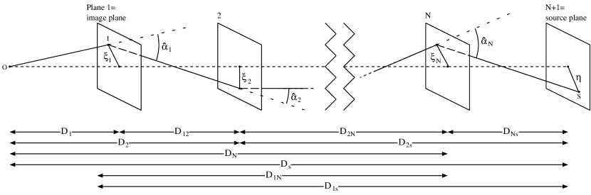
Figure 1: Schematic picture of a multiple lens-plane situation with observer $O$, image $I$ and source $S$.

We start by projecting the mass of each massive object (e.g. galaxy) onto a plane at the respective object redshift. In the $i$:th plane, this gives a surface mass density $\Sigma_{i}({\mbox{\boldmath$\xi$}}_{i})$, where ${\mbox{\boldmath$\xi$}}_{i}$ is the impact parameter of the light-ray in each plane (see figure 1). The justification for this projection is that the light is deflected only in the very vicinity of the lens in most cases and then travels practically unimpeded until it reaches the observer or another lens, situated far away from the preceding one.

2.1.1 The lens equation

From figure 1, where most quantities are defined, we see that the position of the light-ray in each plane can be obtained recursively from the observed position ${\mbox{\boldmath$\xi$}}_{1}$ through

$${\mbox{\boldmath$\xi$}}_{j}=\frac{D_{j}}{D_{1}}{\mbox{\boldmath$\xi$}}_{1}-\sum_{i=1}^{j-1}D_{ij}{\mbox{\boldmath$\hat{\alpha}$}}_{i}({\mbox{\boldmath$\xi$}}_{i}),$$ (1)

where $D_{ij}=D(z_{i},z_{j})$ is the angular diameter distance between redshifts $z_{i}$ and $z_{j}$, $D_{i}=D(0,z_{i})$ and $D_{is}=D(z_{i},z_{\rm source})$. With $N$ lens-planes we find the source position as ${\mbox{\boldmath$\eta$}}={\mbox{\boldmath$\xi$}}_{N+1}$. For convenience we use, in each plane, dimensionless quantities defined by

$${\mbox{x}}_{i}=\frac{{\mbox{\boldmath$\xi$}}_{i}}{\xi_{0i}},$$ (2)

where $\xi_{0i}$ is an arbitrary scale length in the $i$:th plane which, if chosen as $D_{i}$, makes ${\mbox{x}}_{i}$ the angular impact parameter in each plane. Furthermore, the convergence is

$$\kappa_{i}({\mbox{x}}_{i})\equiv\frac{\Sigma(\xi_{0i}{\mbox{x}}_{i})}{\Sigma_{\rm crit}},$$ (3)

where (in geometrised units)

$$\Sigma_{\rm crit}=\frac{D_{s}}{4\pi D_{i}D_{is}}$$ (4)

is called the critical density due to its relation to the ability of a lens to produce multiple images. If we also define ${\mbox{\boldmath$\alpha$}}_{i}={\mbox{\boldmath$\hat{\alpha}$}}_{i}D_{is}/D_{s}$, the scaled deflection potential $\psi_{i}({\mbox{x}}_{i})$, needed for the magnification and defined through ${\mbox{\boldmath$\alpha$}}_{i}=\nabla\psi_{i}$ becomes

$$\psi_{i}({\mbox{x}}_{i})=\frac{1}{\pi}\int_{\mathbb{R}^{2}}\kappa_{i}({\mbox{x}}^{\prime})\ln|{\mbox{x}}_{i}-{\mbox{x}}^{\prime}|\rmd^{2}x^{\prime}.$$ (5)

In these units where ${\mbox{y}}\equiv{\mbox{x}}_{N+1}$ is the source position, the lens equation is given by

$${\mbox{y}}={\mbox{x}}_{1}-\sum_{i=1}^{N}{\mbox{\boldmath$\alpha$}}_{i}({\mbox{x}}_{i}).$$ (6)

2.1.2 The magnification

We now want to find the magnification as a function of image position. Let $A({\mbox{x}}_{1})$ denote the Jacobian matrix of the lens equation

$$A({\mbox{x}}_{1})\equiv\frac{\partial{\mbox{y}}}{\partial{\mbox{x}}_{1}}.$$ (7)

Furthermore we need

$$U_{i}\equiv\frac{\partial{\mbox{\boldmath$\alpha$}}_{i}}{\partial{\mbox{x}}_{i}}=\left(\begin{array}[]{cc}\frac{\partial\alpha_{i1}}{\partial x_{i1}}&\frac{\partial\alpha_{i1}}{\partial x_{i2}}\\ {}\hfil&{}\hfil\\ \frac{\partial\alpha_{i2}}{\partial x_{i1}}&\frac{\partial\alpha_{i2}}{\partial x_{i2}}\end{array}\right)=\left(\begin{array}[]{cc}\psi_{i11}&\psi_{i12}\\ \psi_{i21}&\psi_{i22}\end{array}\right)=$$

$$=\left(\begin{array}[]{cc}\kappa_{i}+\gamma_{i1}&\gamma_{i2}\\ \gamma_{i2}&\kappa_{i}-\gamma_{i1}\end{array}\right),$$ (8)

where

$$\psi_{ikl}=\frac{\partial^{2}\psi_{i}}{\partial x_{k}\partial x_{l}},$$ (9)

$\nabla^{2}_{{\mbox{x}}_{i}}\psi_{i}=2\kappa_{i}({\mbox{x}}_{i})$, $\gamma_{i1}=(\psi_{i11}-\psi_{i22})/2$ and $\gamma_{i2}=\psi_{i12}=\psi_{i21}$. This gives $A$ as

$$A={\mathbb{I}}-\sum_{i=1}^{N}\frac{\partial{\mbox{\boldmath$\alpha$}}_{i}}{\partial{\mbox{x}}_{1}}={\mathbb{I}}-\sum_{i=1}^{N}\frac{\partial{\mbox{\boldmath$\alpha$}}_{i}}{\partial{\mbox{x}}_{i}}\frac{\partial{\mbox{x}}_{i}}{\partial{\mbox{x}}_{1}}={\mathbb{I}}-\sum_{i=1}^{N}U_{i}A_{i},$$ (10)

where ${\mathbb{I}}$ is the 2$\times$2 unit matrix. The $A_{i}$:s can be found by recursion and by noting that $A_{1}={\mathbb{I}}$;

$$A_{j}={\mathbb{I}}-\sum_{i=1}^{j-1}\beta_{ij}U_{i}A_{i}.$$ (11)

Finally, the magnification is given by

$$\mu=\frac{1}{{\rm det}A}=(A_{11}A_{22}-A_{12}A_{21})^{-1}.$$ (12)

Negative values of $\mu$ indicates images of reversed parity relative to the unlensed image.

2.2 Properties of the NFW halo profile

The use of the Navarro-Frenk-White model calls for a brief description of its lensing properties.

Before projection onto the lens plane, the NFW profile is given by

$$\rho_{\rm NFW}(r)=\frac{\rho_{s}}{\frac{r}{r_{s}}\left(1+\frac{r}{r_{s}}\right)^{2}},$$ (13)

where $\rho_{s}$ and $r_{s}$ are scale parameters that can be determined once e.g. the mass is specified, $r$ is the radial co-ordinate. The projected surface mass density will be circularly symmetric and we no longer need vector notation on the impact parameter but instead choose $\xi$ as the radial co-ordinate with the origin at the lens centre. If we choose $\xi_{0}=r_{s}$ (cf. equation (2)) and define $\kappa_{s}=\rho_{s}r_{s}/\Sigma_{\rm crit}$, then

$$\kappa(x)=\frac{2\kappa_{s}}{x^{2}-1}f(x)$$ (14)

where

$$f(x)=\left\{\begin{array}[]{cc}1-\frac{2}{\sqrt{x^{2}-1}}\arctan\sqrt{\frac{x-1}{x+1}}&,x>1\\ 1-\frac{2}{\sqrt{1-x^{2}}}{\rm arctanh}\sqrt{\frac{1-x}{1+x}}&,x<1\end{array}\right.,$$ (15)

and $\kappa(1)=2\kappa_{\rm s}/3$. The deflection angle is

$$\alpha(x)=4\kappa_{s}\frac{g(x)}{x}$$ (16)

where

$$g(x)=\ln\frac{x}{2}+\left\{\begin{array}[]{cc}\frac{2}{\sqrt{x^{2}-1}}\arctan\sqrt{\frac{x-1}{x+1}}&,x>1\\ \frac{2}{\sqrt{1-x^{2}}}{\rm arctanh}\sqrt{\frac{1-x}{1+x}}&,x<1\\ 1&,x=1\end{array}\right.$$ (17)

and the magnification will be given by

$$\mu(x)=\left[\left(1-\frac{\alpha(x)}{x}\right)\left(1+\frac{\alpha(x)}{x}-2\kappa(x)\right)\right]^{-1}.$$ (18)

A flaw of this model is that the total mass diverges when integrated out to infinity. However, this is not too serious since the deflection angle only is sensitive to the mass inside the impact radius, and the magnification is sensitive to this mass and the convergence at this point (for circularly symmetric lenses). Thus all mass outside the impact radius is unimportant.

A single NFW halo gives either one or three images, where the primary image has $\mu\geq 1$, the secondary $\mu<0$ and the tertiary $\mu>0$.

2.3 Properties of the SIS halo

The Singular Isothermal Sphere model, also used here, is based on the assumption that the dark matter in the halo behaves as particles in an ideal gas trapped in their gravitational potential. The gas is assumed to be in thermal equilibrium and the resulting density profile before projection (in geometrised units) is

$$\rho_{\rm SIS}(r)=\frac{\sigma^{2}_{v}}{2\pi r^{2}},$$ (19)

where $\sigma_{v}$ is the line-of-sight velocity dispersion of the particles. If we choose

$$\xi_{0}=4\pi\sigma_{v}\frac{D_{d}D_{ds}}{D_{s}}$$ (20)

the equations for convergence, deflection angle, intrinsic source position and magnification become very simple for this model:

$$\kappa(x)=\frac{1}{2x},$$ (21)

$$\alpha(x)=\frac{x}{|x|}$$ (22)

and

$$y(x)=x-\frac{x}{|x|}$$ (23)

and

$$\mu(x)=\frac{|x|}{|x|-1}.$$ (24)

As with the NFW model, the SIS will give an infinite mass when integrated to infinity but the argument above regarding deflection angle and magnification also holds here. When considering a single SIS halo it can give either one or two images depending on the impact parameter. Primary images have $\mu\geq 1$ and secondary have $\mu<0$.

3 The Q-LET code

The Quick Lensing Estimation Tool, Q-LET is a FORTRAN 77 code written in order to quickly be able to estimate the lensing effects on a point source or an extended object. The structure of the code is as follows

• Read the input datafile and sort the planes

• Check if parameter values are allowed

• Present a choice between a point- or an extended source with elliptical image shape, alternatively a square grid (see section 3.3)

• Compute magnifications and positions of light rays

• Present a choice of how to output the results

A used supplied datafile contains the cosmological parameters, the source redshift and position and the lenses’ redshifts, positions, velocity dispersions or masses and finally their halo type. The mass should be ${\rm M}_{200}$, i.e. the mass within the radius ($\equiv r_{200}$) within which the average energy density is 200 times the critical density at the lens’ redshift.

A point source must be put at the origin. For the case of an elliptical image, the origin will be put at the source centre and the ellipse will be centered at user specified co-ordinates which should be taken as (0,0) if an elliptical image only is studied. The possibility of putting the ellipse off-origin is useful to study e.g. a SN that is offset from its host galaxy centre and the galaxy shape is to be investigated. The SN is put at the origin and the host galaxy central co-ordinates are given as input. If a square grid (see section 3.3) is used, it will be centered at $(0,0)$. The angular positions of the lensing galaxies should of course be assigned with respect to this origin and should be given in arcseconds. The velocity dispersions and masses should be given in ${\rm km}\;{\rm s}^{-1}$ and ${\rm M}_{\odot}$ respectively. See section 3.2 for an example of an input file.

If only ${\rm M}_{200}$ is given for a SIS lens, this mass will be used to calculate the corresponding velocity dispersion since $\sigma_{\rm v}$ is the parameter used to determine the lensing strength for this halo type. If, on the other hand, only $\sigma_{\rm v}$ is given for a NFW lens, this velocity dispersion will be used to calculate the corresponding ${\rm M}_{200}$ for a SIS lens and assuming ${\rm M}_{200}$ is the same for the NFW halo. This is done since the lensing properties of the NFW halo depends upon ${\rm M}_{200}$ in our calculations. If, for some reason, both the mass and velocity dispersion are given, the mass (velocity dispersion) will be ignored for the SIS (NFW) lens.

All distances are computed using the filled beam approximation and it is also with respect to an homogeneous universe that the magnification is given.

3.1 Parameter restrictions

Due to computational complications (and perhaps lack of connection to reality) there are some approximate restrictions on the input parameters. However, these restrictions do not severely limit the usefulness of the code as can be seen in table 1 where the allowed parameter ranges are presented. Furthermore, some of them are not very strict and depends on the values of the other parameters making these ranges approximate only. Especially extremely low or high Hubble parameters ($\sim 0.1$ or $\sim 1.5$ might lead to problems.

Source redshift	$0<z_{\rm s}\lesssim 20$
Lens redshift	$0<z_{\rm l}<{\rm min}[z_{\rm s},5]$
Lens mass $[{\rm M}_{\odot}]$	$10^{6}\lesssim{\rm M}_{200}\lesssim 10^{17}$
Lens velocity disp. $[{\rm km}\;{\rm s}^{-1}]$	5$\lesssim\sigma_{\rm v}\lesssim 5000$
Hubble parameter	$0<h<2$
Mass energy density	$0\leq\Omega_{\rm m}\leq 10$
Energy density in cosmological const.	$-10\leq\Omega_{\Lambda}\leq 10$
Combined restrictions	$\Omega_{\rm m}+\Omega_{\Lambda}=1$ or
when using NFW halo	$\Omega_{\rm m}<1$ and $\Omega_{\Lambda}=0$

Table 1: Approximate parameter restrictions in the code. The Hubble parameter and energy densities are given in units of 100 ${\rm km}\;{\rm s}^{-1}\;{\rm Mpc}^{-1}$ and critical energy density, $\rho_{\rm crit}$ respectively.

3.2 Input

The information needed by Q-LET to be able to compute the magnification and deflection of a light ray is the following: the values of the cosmological parameters, i.e. $h$, $\Omega_{\rm m}$ and $\Omega_{\Lambda}$, the source redshift and position, the lenses’ redshifts and positions, their velocity dispersion or mass and their halo types (NFW or SIS). This information is collected in an input datafile which could have the following appearance:

   0.7     0.3     0.7
   1.7       0       0       0         0  xxxΨ
 0.923    -4.1    3.01     138         0  nfw
 0.655     2.6   -1.11       0      1e12  sis
 0.322   -3.32    5.11       0   9.87e10  nfw
 1.453   -2.32    -0.4   180.0         0  sis
 0.011   -2.34    2.32       0     6.5e9  nfw
 0.234    -4.1    3.01     190         0  sis
 0.254   -5.23   -2.43   100.3         0  nfw

The entries are:
$h_{0}$ $\Omega_{\rm m}$ $\Omega_{\Lambda}$ - - - $z_{\rm source}$ $x_{\rm source}$ [^′′] $y_{\rm source}$ [^′′] 0 0 xxx $z_{{\rm lens}_{1}}$ $x_{{\rm lens}_{1}}$ [^′′] $y_{{\rm lens}_{1}}$ [^′′] $\sigma_{{\rm v}_{1}}$ [${\rm km}\;{\rm s}^{-1}$] ${\rm M}_{{200}_{1}}$ [${\rm M}_{\odot}$] halo type₁ (NFW/SIS) $\vdots$ $\vdots$ $\vdots$ $\vdots$ $\vdots$ $\vdots$ $z_{{\rm lens}_{n}}$ $x_{{\rm lens}_{n}}$ [^′′] $y_{{\rm lens}_{n}}$ [^′′] $\sigma_{{\rm v}_{n}}$ [${\rm km}\;{\rm s}^{-1}$] ${\rm M}_{{200}_{n}}$ [${\rm M}_{\odot}$] halo type_n (NFW/SIS)

For easier handling of the data you should put ’0’ in the fourth and fifth columns and e.g. --- in the sixth column of row 2. Remember to put the source at (0,0) and of course at the highest redshift. The following rows (up to 199 more rows) should contain data on the lensing halos according to the example above.

The program starts by asking for this datafile. The default name is ’qdata.qlet’. In the next step, a question is posed on whether you want to study a point source, an elliptical image or a 20${}^{\prime\prime}\times 20^{\prime\prime}$ square grid. If you choose an elliptical image, you will be asked for another input file with major and minor axes, rotation angle and possible offset from the source (see figure 2). The default name of this input file is ’elldata.ell’ and consists of one line only. An example input file is:
0.8 0.3 72.0 -0.47 0.12
The inputs are $a\ \ b$ in arcseconds, $\varphi$ in degrees and the offset $x^{\prime}$ and $y^{\prime}$ in arcseconds.

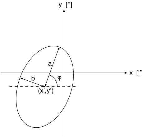
Figure 2: Definitions of major, $a$, minor, $b$, axes, rotation angle, $\varphi$ and offset $x^{\prime}$ and $y^{\prime}$. Units: arcseconds (axes and offset) and degrees (rotation angle).

3.3 Output

If a point source is chosen, it is placed at (0,0) and traced back to the source plane and the magnification is computed. This is printed on the screen, and it is also possible to obtain the output ($x$-, $y$-position and magnification) in a small file. If a magnification $\mu<1$ is obtained, it is not a primary image that has been found, i.e. muliple imaging has occurred. In the case of an elliptical image, the user is asked to provide the number of the plane wished to be output in a file. You can choose any plane between 2 and the number of the source plane if you would like to study the intermediate changes of the ray bundle. Each row in the output file refers to a specific ray and could look like:
8395. 0.2131891 0.8527565 -2.296262 0.633064 2.873963
The entries are:
No. of the ray $x_{1}$ [^′′] $y_{1}$ [^′′] $x_{i}$ [^′′] $y_{i}$ [^′′] magnification,
where subscript 1 refers to the image plane and $i$ refers to the chosen plane. The file will contain a quite large amount of rays in order to see the shape better (of order 1-5$\times 10^{4}$, depending on the size of the ellipse). To see the result, just plot the file with the desired columns.

When a square grid is chosen, the output file will look exactly like in the ellipse-case, the difference is that the grid is square and pre-defined to be 20${}^{\prime\prime}\times 20^{\prime\prime}$. This grid can be used if the image(s) has (have) a shape not described by an ellipse. When trying to estimate the intrinsic shape of an object like this, you plot the 4:th and 5:th columns making cuts using the 2:nd and 3:rd columns as to only include the rays making up the image(s). If instead wishing to see e.g. what an intrinsically elliptical source looks like in the image plane, you make the cut using the 4:th and 5:th columns, even though the grid in the source plane is not evenly distributed it will be possible as long as it covers the area where the cut is made.

4 Example: application to SN2003es

SN2003es was found at a redshift of 0.968 in the Hubble Deep Field North (HDF-N) in April 2003 by the GOODS/HST Transient Search, as part of the HST Treasury program [29]. As the host galaxy seems to be an elliptical, it is most likely a Type Ia SN [30]. Since these are used as standard candles to determine the redshift-distance relation in the quest for the cosmological parameters, it is very important to study the potential magnification by gravitational lensing. There are several possible lens candidates close to the line-of-sight of SN2003es so a close inspection is necessary.

4.1 Host and lensing galaxy data

The data on the host and lens galaxies has been taken from three different references; [31, 33, 34]. Since the redshift information differ significantly in the different catalogs, we used the principle to take the spectroscopic redshifts when available and the photometric redshifts otherwise. If two catalogs had only photometric redshifts, the most recent result was used. However, as a worst case scenario regarding the amount of magnification, we also computed the magnification including four galaxies from one of the older catalogues which, in the most recent catalogue, were determined to be background galaxies at $z>z_{\rm source}$. Hereafter we call these GH after Gwyn and Hartwick of reference [33].

To estimate the velocity dispersion that is needed in the lensing calculation, we took the observed luminosities and best fit galaxy morphology from [31] and performed cross-filter K-corrections to rest frame $B_{J}$ using galaxy templates provided by the SNOC package [32]. The Tully-Fisher (T-F) relation for spirals (Sxx) and Faber-Jackson (F-J) relation for ellipticals (Ell) and irregulars (Irr) were used to derive an approximate velocity dispersion. The relations are given by

$$\frac{\sigma_{\rm v}}{\sigma_{*}}=10^{0.088(M_{*}-M)}\ \ \ \ \ ({\rm T-F})\\$$ (25)

and

$$\frac{\sigma_{\rm v}}{\sigma_{*}}=10^{0.1(M_{*}-M)}\ \ \ \ \ \ \ \ ({\rm F-J}),$$ (26)

where $\sigma_{*}$ is the normalisation of the velocity dispersion, $M$ is the absolute magnitude in $B_{J}$ and $M_{*}$ is a typical magnitude taken to be $M_{*}=-19.53+5\log h$ [35].

Within a radius of 10^′′ we found 9 lensing galaxies excluding GH and 13 lenses including it. The redshifts, velocity dispersions, positional data and galaxy types can be found in table 2.

Cat. no	$z$	$x$-pos. $[^{\prime\prime}]$	$y$-pos. $[^{\prime\prime}]$	$\sigma_{\rm v}/\sigma_{*}$	Gal. type
526	0.120	-3.74	-8.60	0.136	Scd
539	0.120	-2.55	-7.93	0.112	Scd
549	0.952a	1.62	-8.29	0.924	Ell
622	0.440	4.76	-2.59	0.332	Scd
623	0.960	-6.80	2.58	0.334	Scd
631	0.321a	1.69	-0.52	0.460	Irr
662	0.511a	2.71	2.88	0.557	Irr
693	0.600	2.52	6.85	0.402	Ell
700	0.040	-1.52	9.28	0.098	Sbc
GH galaxies
582	0.904	-9.73	-0.62	0.401	Scd
607	0.776	1.64	-3.07	0.431	Sbc
610	0.296	0.87	-2.43	0.218	Scd
696	0.904	8.52	4.51	0.682	Irr
Host galaxy
619	0.968a	-0.475	-0.710	(1.290)	Ell

Table 2: Lensing galaxy data. The galactic centre position is given relative to the co-ordinates of SN2003es. The galaxy type is the best fit from reference [31]. The galaxies with spectroscopically determined redshifts are superscripted $a$.

4.2 Results

We used the Q-LET code to compute the magnification of SN2003es and also to find the intrinsic shape of the host galaxy. This is done in order to see that the observed elliptical shape is not contrived from an intrinsically very complicated shape that is never observed in reality. The normalisation of the velocity dispersion is quite poorly known [36] and we choose to present the magnification as a function of this normalisation. For the host galaxy shape calculation we used a value of $\sigma_{*}=170$ km/s, obtained as an average in reference [37] for a mixture of galaxy morphologies. However, the shape is not distorted very much even with $\sigma_{*}$ as high as 300 km/s, although it is translated and more strongly magnified. The result on the magnification is found in figure 3. We have used models where all halos are assumed to be either of NFW or SIS type. The figure also shows the result both when including the four GH galaxies and when excluding them. As is seen, in the region of $\sigma_{*}$ between 150 and 200 km/s, i.e. around 170 km/s, the magnification varies between roughly 1.08 and 1.27 depending on the the model and the presence of the GH galaxies. This corresponds to a magnitude shift of $0.1\lesssim\Delta m\lesssim 0.25$ mag, a significant change that could dominate the uncertainty (the intrinsic magnitude spread in Type Ia SNe is roughly between 0.1 and 0.2 mag [38]). Note also that higher $\sigma_{*}$ have been obtained e.g. in reference [39], where a value for the SIS of roughly 275 km/s was obtained for the dark matter in ellipticals.

Figure 3: Magnification of SN2003es as a function of the velocity dispersion normalisation.

In figure 4, we display the intrinsic (unlensed) position relative to the observed position at (0,0), depending on $\sigma_{*}$ and the model (NFW/SIS and GH incl./GH excl.). We see that the shift is only weakly depending on the halo type for this lens system under our assumptions.

Figure 4: The intrinsic (unlensed) position of SN2003es relative to the observed position at (0,0). The position will move along the curves from left to right with increasing $\sigma_{*}$ as indicated.

Finally, we show the intrinsic shape of the host galaxy for a $\sigma_{*}$ of 170 km/s [37] in figure 5. This plot also shows the small difference in deflection between NFW and SIS halo models under our assumptions. The shapes were computed including the GH galaxies. The axis ratios of both the NFW and SIS case are roughly 0.9, making them perfectly normal E1 galaxies so no constraints on the magnification or model can be inferred from the host galaxy shape.

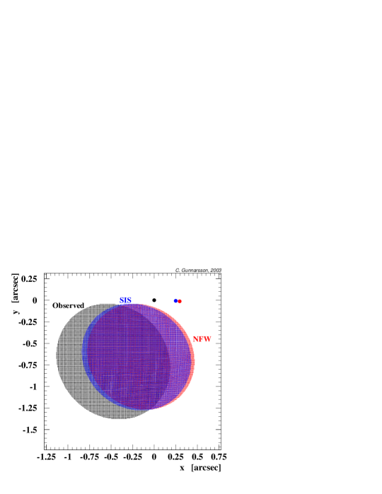
Figure 5: The observed and intrinsic shapes of the host galaxy. The larger dots indicate the position of the supernova. The figure shows the small difference in deflection between NFW and SIS halo models under our assumptions.

5 Discussion — Q-LET & SN2003es

One of the approximations that may be criticised is the fact that we extend the halos out to infinity. However, the lensing effect at large impact radii is very small. For SN2003es, the lenses with large impact radii contribute very little to the total magnification which is dominated by galaxies no. 631 and 662.

Putting ${\rm M}_{200}$ of the NFW equal to that of the SIS for a given velocity dispersion is not obviously a good approximation. The most likely measured quantities are the luminosity or velocity dispersion of the lens and the luminosity may be used to estimate a velocity dispersion either via the Tully-Fisher or Faber-Jackson relation. When a velocity dispersion is obtained, the best way would be to use it directly on the NFW profile. However, as opposed to the SIS, the NFW velocity dispersion depends on the radius. By following Łokas and Mamon in reference [28] it is possible to obtain the line-of-sight velocity dispersion, $\sigma_{\rm los}$, for well resolved sources, or, for small or distant sources, the “aperture velocity dispersion”, $\sigma_{\rm ap}$, which is the average over an aperture centered on the object. We calculated both these quantities as a function of radius and found that $\sigma_{\rm ap}$ did not fall off dramatically. As an example, in a case where we put the SIS velocity dispersion ($\sigma_{\rm v}^{\rm SIS}$) to 170 km/s to get the parameters for the NFW and then compute the corresponding NFW velocity dispersions, $\sigma_{\rm ap}$ varies roughly by $+5$% and $-15$% around 170 km/s between radii $0.1r_{200}$ and $2r_{200}$. The line-of-sight velocity dispersion varies more, $+10$% to $-40$% in the same range. However, at a radius of roughly $0.3r_{200}$, there is a quite small scatter around the SIS value of less than $\sim$15%. This seems to be valid for a large range of redshifts and velocity dispersions. It also seems valid in low $H_{0}$- and low density universes. Thus in almost all cases it is possible to find a radius at which $\sigma_{\rm los}\sim\sigma_{\rm ap}\sim\sigma_{\rm v}^{\rm SIS}$, with this radius being roughly equal to $0.3r_{200}$.

Inverting the velocity dispersion-mass relation for the NFW is quite time-consuming, and this, along with the ambiguity due to the dependence of $\sigma_{\rm v}$ on radius and the fact that the difference seems not to be significant, motivates using the simpler conversion via the SIS. However, if this conversion is unsatisfactory, it is always possible for the user to supply ${\rm M}_{200}$ instead, in which case of course no conversion is needed.

For the irregular galaxies we have used the Faber-Jackson relation which is valid for ellipticals. An approximation which is difficult to say to what extent it affects the results, and in which direction. Using the Tully-Fisher relation on the irregulars would increase the magnification even further, but at most by $\sim$15-20%.

Whether the halo models we use are good descriptions of real halos is still under debate. We are using spherically symmetric models, which might be an oversimplification but the ellipticity of the dark matter in the observed halos is in practice very seldom known (see e.g. reference [40] for the effects of ellipticity in lensing).

So, unless some new model is very different from the SIS and NFW, the results for SN2003es is likely to remain.

5.1 Conclusions

We have found that SN2003es is likely to have been significantly magnified by gravitational lensing, a fact that must be taken into account when trying to use this (likely Type Ia) SN to infer cosmological parameters. Either a more thorough analysis of the lensing galaxies is needed to take the effect into account or the SN should be used only to set a lower limit on the distance or maybe even be excluded from the sample if not having large statistics. In that case some SNe are likely to be de-magnified and the effect can be assumed to average to $\sim 0$. The fact that the intrinsic shape of the host galaxy looks perfectly normal makes it practically impossible to use this shape to put constraints on the magnification of SN2003es. If an extremely unusual shape would have been obtained, it could perhaps have affected the reliability of the model.

6 Summary

We have presented the multiple lens-plane method of gravitational lensing along with its implementation in Q-LET, a FORTRAN 77 code that can be used to quickly estimate the lensing effects on either a point source or to obtain the intrinsic shape of an elliptical image. A square grid in the image plane is also possible for user-defined image shapes.

The code was applied to SN2003es, a SN (most likely Type Ia) discovered in the HDF-N. Using both NFW and SIS type halos and estimating the velocity dispersions from the observed luminosities via the Faber-Jackson and Tully-Fisher relations we found that SN2003es is likely to have been significantly magnified by gravitational lensing and that this problem should be addressed in detail before using SN2003es in estimates of the cosmological parameters.

References

References

- [1] D N Spergel et al., 2003 Astrophys. Jour. Suppl. 148 175
- [2] C L Kuo et al., submitted to ApJ [astro-ph/0212289]
- [3] T J Pearson et al., 2003 ApJ 591 556
- [4] W J Percival et al., 2001 Mon. Not. Roy. Astr. Soc. 327 1297
- [5] R A C Croft et al., 2002 ApJ 581 20
- [6] N Y Gnedin and A J S Hamilton, 2002 MNRAS 334 107
- [7] S Perlmutter et al., 1999 ApJ 517 565
- [8] A G Riess et al., 1998 Astronom. Jour. 116 1009
- [9] M M Phillips,1993 ApJ 413 L105
- [10] S Perlmutter et al., 1997 ApJ 483 565
- [11] P de Bernardis et al., 2002 ApJ 564 559
- [12] M E Abroe et al., 2002 MNRAS 334 11
- [13] A Goobar, L Bergström and E Mörtsell, 2002 Astron. &Astrophys. 384 1
- [14] A Aguirre,1999 ApJ 512 L19
- [15] A Aguirre, 1999 ApJ 525 583
- [16] H Umeda, K Nomoto, C Kobayashi, I Hachisu and M Kato, 1999 ApJ 522 L43
- [17] P Höflich, K Nomoto, H Umeda and J C Wheeler, 2000 ApJ 528 590
- [18] I Domínguez, P Höflich and O Straniero, 2001 ApJ 557 279
- [19] M Sullivan et al., 2003 MNRAS 340 1057
- [20] E Mörtsell and A Goobar, 2003 Jour. of Cosm. and Astropart. Phys. 0304 003
- [21] R Amanullah, E Mörtsell and A Goobar, 2003 A&A 397 819
- [22] G F Lewis and R A Ibata, 2001 MNRAS 324 L25
- [23] E Mörtsell, C Gunnarsson and A Goobar, 2001 ApJ 561 106
- [24] A G Riess et al., 2001 ApJ 560 49
- [25] N Benítez et al., 2002 ApJ 577 L1
- [26] L-X Li and J P Ostriker, 2002 ApJ 566 652
- [27] P Schneider, J Ehlers and E Falco, 1992 Gravitational Lenses (Berlin: Springer verlag)
- [28] E L Łokas and G A Mamon, 2001 MNRAS 321 155
-
[29]
L G Strolger, GOODS Treasury Team, 2003 IAU
Circ.8140 1
see also: http://www.stsci.edu/ftp/science/goods/transients.html - [30] S van den Bergh and G A Tammann, 1991 Ann. Rev. of Astron. & Astrophys. 29 363
-
[31]
A Fernández-Soto, K M Lanzetta and A Yahil, 1999 ApJ
513 34
see also: http://bat.phys.unsw.edu.au/~fsoto/hdfcat.html - [32] A Goobar et al., 2002 A&A 392 757
-
[33]
S D J Gwyn and F D A Hartwick, 1996 ApJ 468
L77
see also: http://astrowww.phys.uvic.ca/grads/gwyn/pz/hdfn/ - [34] J G Cohen et al., 2000 ApJ 538 29
- [35] P J E Peebles, 1993 Principles of Physical Cosmology (Princeton: Princeton University Press)
- [36] G Wilson, N Kaiser, G A Luppino and L L Cowie, 2000 ApJ 556 601
- [37] P Fisher et al., 2000 AJ 120 1198
- [38] M Hamuy et al., 1996 AJ 112 2391
- [39] M Fukugita and E L Turner, 1991 MNRAS 253 99
- [40] C R Keeton, C S Kochanek and U Seljak, 1997 ApJ 482 604