Collapse of Magnetized Singular Isothermal Toroids: I. Non-Rotating Case

Abstract

We study numerically the collapse of non-rotating, self-gravitating, magnetized, singular isothermal toroids characterized by sound speed, $a$, and level of magnetic to thermal support, $H_{0}$. In qualitative agreement with previous treatments by Galli & Shu and other workers, we find that the infalling material is deflected by the field lines towards the equatorial plane, creating a high-density, flattened structure – a pseudodisk. The pseudodisk contracts dynamically in the radial direction, dragging the field lines threading it into a highly pinched configuration that resembles a split monopole. The oppositely directed field lines across the midplane and the large implied stresses may play a role in how magnetic flux is lost in the actual situation in the presence of finite resistivity or ambipolar diffusion. The infall rate into the central regions is given to 5% uncertainty by the formula, $\dot{M}=(1+H_{0})a^{3}/G$, where $G$ is the universal gravitational constant, anticipated by semi-analytical studies of the self-similar gravitational collapses of the singular isothermal sphere and isopedically magnetized disks. The introduction of finite initial rotation results in a complex interplay between pseudodisk and true (Keplerian) disk formation that is examined in a companion paper.

1 Introduction

1.1 Low-Mass Star-Formation Theory

Stars form in the dense cores of molecular clouds (Myers 1995, Evans 1999). The nearby cores that form low-mass stars have a typical diameter $\sim$ 0.1 pc, a number density $\sim 3\times 10^{4}$ cm^-3, a mass ranging from a fraction of a solar mass to about 10 $M_{\odot}$, and an axial ratio for flattening of typically 2:1. Agents other than isotropic thermal or turbulent pressures must help to support cores against their self-gravity, although there is some debate whether the true shapes are oblate, prolate, or triaxial (Myers 1998, personal communication; see also Jones & Basu 2002). Observed cloud rotation rates are generally too small to account for the observed flattening (Goodman et al. 1993), and tidal effects from neighboring cores cannot explain the flattening of inner density contours. This leaves magnetic fields, implicated in many other physical processes of importance in contemporary star formation (see the reviews of Shu et al. 1987, 1999).

In one scenario, ambipolar diffusion leads to a continued contraction of a cloud core with ever growing central concentration (Nakano 1979, Lizano & Shu 1989, Basu & Mouschovias 1994). In a finite time given by slippage of neutrals past ions and magnetic fields, the molecular cloud core reaches a configuration where the central density formally tries to reach infinite values. Shu (1995) proposed the name “gravomagneto catastrophe” for this mechanism by analogy with the “gravothermal catastrophe” (Lynden-Bell & Wood 1968, Lynden-Bell & Eggleton 1980, Cohn 1980) that overtakes globular-cluster core-evolution because of the diffusion of random velocities by stellar encounters.

Myers (1999) has emphasized that inward fluid velocities of magnitude $\sim 0.1$ km s^-1 exist at large radii in some starless cores, and that this feature is not predicted by any of the ambipolar-diffusion calculations cited above (see, however, Li 1998a and Ciolek & Basu 2000). Myers & Lazarian (1998) suggest instead that pre-existing inward motions prior to true gravitational collapse and star formation are better modeled as resulting from the decay of turbulence. If the sequence of decaying turbulent parameter $K=12,10,6,2$ in Figure 2 of Lizano & Shu (1989) were to occur over $\sim$ a few Myr, then inward motions of order half the isothermal sound speed, $0.5a\sim$ 0.1 km s^-1, could indeed be generated at distances of order $0.1$ pc from the center of the cloud core. Large-scale inward motions and generally shorter time scales may distinguish the “gravoturbo catastrophe” resulting from the decay of turbulence in a pre-existing, magnetically supercritical, core with dimensionless mass-to-flux ratio $\lambda>1$ (see Li & Shu 1966 for the definition of $\lambda$) from a core that reaches supercriticality via ambipolar diffusion. As we shall see later, inclusion of initial inward motions of order $0.5\,a$ increases the net central mass-accretion rate due to subsequent gravitational collapse by about a factor of 2.

1.2 The Pivotal State

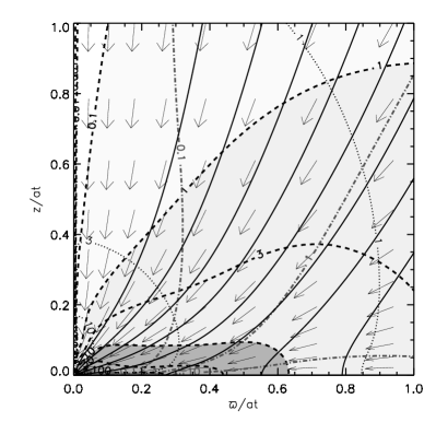
Figure 7: Collapse solution of the $H_{0}=0.25$ case with an initial inward radial velocity of $0.5a$. The contours of constant self-similar density $4\pi Gt^{2}\rho$ are plotted as dashed lines, with the shades highlighting the high density regions. The magnetic field lines are plotted as solid lines, with contours of constant $\beta$ (dash-dot-dashed) superposed. The velocity in every fifth cell is shown by unit vectors, with its magnitude in units of the sound speed given by the dotted contours.

Li & Shu (1996) termed the cloud configuration when the central isothermal concentration first becomes formally infinite as the “pivotal” state ($t\equiv 0$). This state separates the nearly quasi-static phase of core evolution ($t<0$) that leads to gravomagneto or gravoturbo catastrophe ($t=0$) from the fully dynamic phase of protostellar accretion ($t>0$). (See the first two stages depicted in Fig. 7 of Shu, Adams, & Lizano 1987.) The numerical simulations indicate that the pivotal states have a number of simplifying properties, which motivated Li & Shu to approximate them as scale-free equilibria with the power-law radial dependences for the density and magnetic flux function:

$$\rho(r,\theta)={a^{2}\over 2\pi Gr^{2}}R(\theta),\qquad\Phi(r,\theta)={4\pi a^{2}r\over G^{1/2}}\phi(\theta).$$ (1)

In equation (1), we have adopted a spherical polar coordinate system $(r,\theta,\varphi)$, and $a$ is the isothermal sound speed of the cloud, while $R(\theta)$ and $\phi(\theta)$ are the dimensionless angular distribution functions for the density and magnetic flux given by force balance along and across field lines. The resulting differential equations and boundary conditions yield a linear sequence of possible solutions, characterized by a single dimensionless free parameter, $H_{0}$, which represents the fractional over-density supported by the magnetic field above that supported by thermal pressure. Comparison with the typical degree of elongation of observed cores suggests that the over-density factor $H_{0}\approx 0.5-1$ (corresponding to $\lambda\approx 2$).

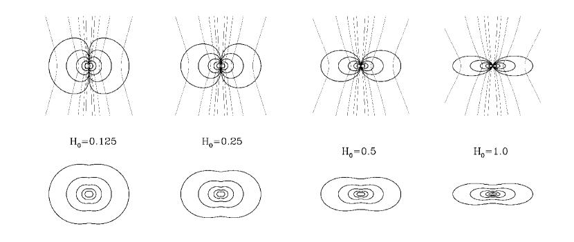
Figure 1: Top: Isodensity contours and magnetic field lines for a few selected values of $H_{0}$. Bottom: Equatorial plane projection of the column density (taken from Shu et al. 1999).

In Figure  1, we plot isodensity contours and field lines for the cases $H_{0}$ = 0.125, 0.25, 0.5, 1.0. The corresponding values of $\lambda$ from Table 1 of Li & Shu (1966) are $\lambda$ = 8.38, 4.51, 2.66, 1.79. Below each case are the column density contours that would be seen by an observer in the equatorial plane of the configuration. The presence of very low-density regions at the poles of the density toroid has profound implications for the shape and kinematics of bipolar molecular outflows (Li & Shu 1996, see also Torrelles et al. 1983, 1994).

1.3 Self-Similar Collapse of Singular Isothermal Toroids

It is well-known that the collapse of the singular isothermal sphere (corresponding to the case $H_{0}=0$ in the previous section) occurs in a self-similar manner (Shu 1977). The same holds true for any member in the sequence of isopedically magnetized, singular isothermal toroids (SITs), whether we start them from rest, or with a initial, radially directed, velocity field that is a uniform fraction of the isothermal sound speed $a$. For given $H_{0}$, we have only two dimensional parameters in the problem, $a$ and $G$. From $a$ and $G$, we cannot form dimensions for all required physical quantities without using the independent variables of the problem themselves: $r$, $\theta$, and $t$. The quantities $r$ and $at$ both have the dimensions of length, and they can be combined to form the dimensionless similarity variable

$$x=r/at,$$ (2)

which can then appear, along with $\theta$, as the argument for nondimensional mathematical functions. Thus, the time-dependent axisymmetric solution that describes the $t>0$ evolution of the unstable equilibrium state (1) must take the self-similar form:

$$\rho(r,\theta,t)={\alpha(x,\theta)\over 4\pi Gt^{2}},\;\;{\bf u}(r,\theta,t)=a{\bf v}(x,\theta),\;\;{\bf B}(r,\theta,t)={a\over G^{1/2}t}{\bf b}(x,\theta),$$ (3)

where $\bf u$ and $\bf B$ are the poloidal fluid velocity and magnetic field, respectively. The dimensionless dependent variables $\alpha(x,\theta)$, ${\bf v}(x,\theta)$, and ${\bf b}(x,\theta)$ are called the reduced density, velocity, and magnetic field. Solutions with the form (3) are called “self-similar” because, apart from a simple scaling of dependent and independent variables, the solution at one instant in time looks the same as the solution at another instant in time.

For the case $H_{0}$ = 0 (corresponding to ${\bf b}=0$), we may assume that the flow occurs spherically symmetrically. With no $\theta$ dependence and with ${\bf v}$ having only a radial component, the similarity solution has a simple description if the SIS is started from rest (Shu 1977). At $t=0^{+}$, consider initiating collapse of the densest innermost portions of a (nonrotating and unmagnetized) singular isothermal sphere to form a condensed central object (a protostar, whose physical dimensions are so small as to allow us here to approximate it as a point mass). An observer located in the outer portions of the cloud does not realize anything has happened gravitationally, because Newton’s theorem for the gravitational field of spherical objects misleads the observer into thinking that all the mass interior to the observer’s location equivalently lies at the center anyway. Only when a sound wave traveling outwards at the speed $a$ reaches the observer, does the observer realize, hydrodynamically, that the bottom has dropped out. This information initiates a wave of falling whose location at time $t$ has a head described by the locus $r=at$. The similarity variable description for the same locus is $x=1$. For $x$ larger than 1 (or $r>at$), the density profile retains its unperturbed value $\alpha=2/x^{2}$ (or $\rho=a^{2}/2\pi Gr^{2}$), and the fluid is at rest, ${\bf v}=0$ (or ${\bf u}=0$).

The solution interior to the head of the expansion wave is modified from the initial equilibrium. At $x$ = 1, the solutions for $\alpha$ and $v$ connect without a jump, but with a discontinuous first derivative (because of the presence of the head of the wave) to the unperturbed state corresponding to the singular isothermal sphere. Near the origin, the solutions take the asymptotic forms,

$$\alpha\rightarrow\left[{m_{0}\over 2x^{3}}\right]^{1/2},\qquad v(x)\rightarrow-\left[{2m_{0}\over x}\right]^{1/2},\qquad{\rm as}\qquad x\rightarrow 0,$$ (4)

that correspond to gravitational free-fall onto a (reduced) central mass found by numerical integration to be $m_{0}=0.975$. In dimensional units, the origin contains a central mass point (star) that grows linearly with time:

$$M=m_{0}{a^{3}t\over G}.$$ (5)

Equation (5) constitutes the most important property of the solution – the conclusion that the gravitational collapse of a singular isothermal sphere yields, not a characteristic mass, but a characteristic mass infall rate given by

$$\dot{M}=m_{0}\,{a^{3}\over G}.$$ (6)

Inclusion of the effects of finite levels of the magnetic field (i.e., $H_{0}\neq 0)$ does not change the qualitative situation. The collapse still occurs self-similarly from “inside-out,” but the departures from spherical symmetry implies that non-zero motions can be induced gravitationally ahead of the front of an expansion wave (see also Terebey, Shu, & Cassen 1984 for the case when the cause of departure from spherical symmetry is rotation). If the gravitational precursor motions are sufficiently compressive, the expansion wave, now propagating outward at the fast MHD speed, may even be preceded by a weak shock wave (Li & Shu 1997). But the main new feature introduced by the presence of the magnetic field is a flattening of the flow in the inner regions to form a “pseudodisk” (see the singular perturbational treatment by Galli & Shu 1993a,b of this problem). We will concentrate on the formation and structure of this pseudodisk in our numerical calculations, and we shall focus for simplicity most of our attention on equilibrium configurations started from rest. At the end, however, we will discuss the modifications introduced by starting with uniform inward motions present already at the pivotal instant.

Strict field freezing implies that the mass-to-flux ratio is a conserved quantity: $\lambda$ = const. Except for the time-dependent behavior that tapers the surface density distribution near the edge, pseudodisks formed from the gravitational collapse of magnetized SITs therefore will resemble nonrotating, magnetized, singular isothermal disks with values of the dimensionless mass-to-flux ratio $\lambda$ greater than, but close to, unity. Since such disks, started from rest, collapse to yield a central mass-accretion rate $\dot{M}=m_{0}a^{3}/G$ with $m_{0}=1.05(1+H_{0})$, Li & Shu (1997) speculated that magnetized SITs, for arbitrary initial values of $H_{0}$ from 0 to $\infty$, would develop central mass-infall rates well-approximated (to 5% accuracy) by the simple formula:

$$\dot{M}=(1+H_{0}){a^{3}\over G},$$ (7)

where $H_{0}$ is the degree of support by magnetic fields provided in the pivotal configuration. One of the major goals of the present numerical simulation is to justify explicitly the above equation.

For $a\approx 0.2$ km s^-1 and $H_{0}\approx 0.5$ (Taurus region), equation (7) yields $\dot{M}\approx 3\times 10^{-6}$ $M_{\odot}$ yr^-1, in agreement with the spectral energy distribution (SED) and light-scattering models of Kenyon et al. (1993a, b). The time $t$ required to build the typical T Tauri star of mass 0.5 $M_{\odot}$ is then $1.7\times 10^{5}$ yr. The inference of constant accretion rates, with associated mass-accumulation time scales of $\sim 10^{5}$ yr and observed luminosities according to standard models of protostellar evolution (e.g. Stahler et al. 1980, Palla & Stahler 1990), is consistent with the survey of Hirano et al. (2002) of 17 protostellar sources in isolated dark clouds, Taurus, and Rho Ophiuchus star-forming regions. They are not consistent with claims for coefficients in the relationship, $\dot{M}\propto a^{3}/G$, which are either one to two orders of magnitude larger or highly time-variable, that have been claimed in the literature based on numerical simulations (for low-mass star-forming regions) starting from conditions rather different from singular isothermal toroids (see, e.g., Tomisaka 2002, who started the collapse calculation from an infinitely long cylinder, with the collapse induced by a sinusoidal perturbation in density along its length). Myers & Fuller (1993; see also Myers, Ladd, & Fuller 1991; Myers 1995) made the intriguing suggestion that total mass-accumulation time scales $\sim 10^{5}$ yr may apply across the board, from the formation of the lowest-mass to the highest-mass stars. If this suggestion has merit, and if we continue to use static, magnetized SITs to model the pivotal states of such objects, then the final mass of the formed star must scale with the factor $a^{3}(1+H_{0})$, with this factor being larger to form more massive stars. In other words, massive star-forming regions must be hotter, or more highly magnetized, or more turbulent (if we heuristically include the effect of turbulent support into $H_{0}$), than low-mass star-forming regions (see the reviews of Shu et al. 1987 and Evans 1999).

Non-isothermal equations of state to mimic the effects of turbulence (where the signal speeds are larger at lower densities) can yield pivotal states with density laws that are shallower than the $\rho\propto r^{-2}$ dependences that are considered in this paper (see, e.g., Lizano & Shu 1989, McLaughlin and Pudritz 1997, Galli et al. 1999). The gravitational collapse of such non-isothermal configurations will yield mass infall rates $\dot{M}$ that increase with time. In contrast, pre-existing inward motions in the central region at the pivotal instant $t=0$ tend to yield $\dot{M}$ that decreases with time (Basu 1997, Ciolek & Königl 1998, Li 1998a). When added to the support provided quasistatically by thermal pressure, all of these mechanisms enhance the mass infall rate above the base value given by the inside-out collapse solution for the initially static, singular isothermal sphere: $\dot{M}=0.975a^{3}/G$. None of the considerations imply that $\dot{M}$ should cut off after some definite time and leave us with a star with a well-defined mass. We return to this difficulty in the last section of this paper (see also the discussion in Shu & Terebey 1984, Shu et al. 1999).

In any case, whether or not ideally magnetized SITs represent good pivotal states at $t=0$ for star formation models, the self-similar nature of their $t>0$ behavior greatly simplify both the collapse calculations and data storage requirements. For the latter, we need to store the reduced variables that are only functions of the similarity coordinates $(x,\theta)$. Moreover, these reduced variables depend only on a single dimensionless parameter $H_{0}$ of the initial state (deducible under the assumption of field freezing from a measurement of $\lambda$ at any instant during the dynamical collapse). Comparisons with the variables of actual observations at any dimensional time $t$ can then be obtained from the single parameter family of solutions by appropriate scalings of dependent and independent variables by various factors of $t$, $a$, and $G$.

2 Numerical Method and Simulation Setup

We follow the inside-out collapse of magnetized singular isothermal toroids using Zeus2D (Stone and Norman, 1992a,b), which solves the ideal MHD equations in 3 dimensions with an axis of symmetry. Ideal MHD is a reasonable approximation during the dynamic collapse, since there is little time for the magnetic field to diffuse outwards relative to the bulk matter (see, e.g., Galli & Shu 1993a, b). We are interested in the dynamics of the collapsing flow not too close to the center, where IR radiation can escape freely and an isothermal equation of state can be adopted. We note that violation of the isothermal assumption could affect the vertical structure of pseudodisks, which may be bounded by accretion shocks on their upper and lower surfaces.

Zeus2D is a well tested, general purpose, publicly available package. Applying it to our specific problem was not without difficulties. These difficulties and the modifications we developed to overcome them are discussed below.

2.1 Polar Axis and Central Cell Modifications

The family of models studied in this paper suffers from several numerically inconvenient features, including a point mass at the origin that grows linearly with time and a near vacuum in the polar region. The near-vacuum region is further complicated by finite magnetic field strengths that imply nearly infinite Alfvén speeds. Close to the polar axis, field lines run nearly parallel to the polar axis so that there is little (vertical) magnetic support of fluid. With an increasing point mass at the origin, velocities grow and densities deplete with time. Small irregular Lorentz forces induced by a wave traveling up a field line can produce artificially large fluid velocities in the near vacuum that cause the cell to deplete faster than gravity can actually draw down the gas.

We allow mass to accumulate in the central cell, and modify the ZEUS code so that only equations dealing with magnetic fields see the matter in the central cell. Particularly, the large pressure in the central cell is ignored in computing pressure gradients in the force equation, as in the standard sink-cell method. The central cell itself does not appear to cause any numerical problem. Those close to the origin along the polar axis are, however, vulnerable to instability. Usually, one cell would become depleted of fluid so that either the Alfvén speed would become too large (in strong field cases) or fluid velocities would become infinite (weak field cases). The instability is purely numerical; a vacuum moving at infinite speeds is physically meaningless. The representation of a spherical singularity by a cylindrical central cell may aggravate the difficulties, eventually halting the simulation. In some cases, we could mitigate this instability by imposing the monopole solution for velocity (Galli & Shu, 1993a,b) along the polar axis region where $x<0.1$. The corrections change only the features of the near vacuum region around the polar axis and have no influence on other regions of physical interest in the simulation.

2.2 Alfvén Limiter in Low Density Polar Region

For the magnetized singular isothermal toroids, which are the initial configurations of our simulations, the magnetic field close to the polar axis scales as $B\propto 1/r$. The density close to the polar axis scales as $\rho\propto\theta^{4H_{0}}/r^{2}$. Thus, the Alfvén speed near the polar axis, $v_{a}\propto|B|/\sqrt{\rho}\propto\theta^{-2H_{0}}$, becomes increasingly divergent as $H_{0}$ increases. The maximum timestep in an explicit code such as Zeus2D is limited by the Courant condition, which sets the maximum timestep to be of order the fastest cell-crossing time of Alfvén wave for all the cells. Thus, as $H_{0}$ increases, the maximum timestep $\Delta t\propto\theta^{2H_{0}}$ becomes increasingly small for cells close to the polar axis, creating a problem for the simulations.

We circumvent the Alfvén problem by artificially decreasing the Alfvén speed when the speed becomes too high. This fast Alfvén impediment to MHD simulations is not new. One method to overcome the problem that has had some success (Miller & Stone, 2000), involves inclusion of the displacement current in Maxwell’s induction equation, but with a reduced value for the speed of light (Boris, 1970). This sets an upper bound to the Alfvén speed. We note that the use of the Alfvén limiter does not destroy the self-similarity of the problem as long as we set the speed of light equal to a constant multiple of the speed of sound $a$. Of course, there is a price to pay for the larger timestep possible; one can not expect accurate results in regions where the Alfvén speed has been truncated (e.g. near the polar axis). This price is worth paying, as demonstrated below.

2.3 Boundary Conditions and Grid

Aside from the Courant condition, a more subtle issue with the boundary conditions required the Alfvén limiter to be imposed for our simulations. Outer boundary conditions were set either to be divergence-free outflow (important for the rotating cases to be discussed in our companion paper) or calculated from the fluid variables at an earlier time $\tau$ and smaller radius within the computational domain by use of the self-similarity of the problem:

$$\rho(r,\theta,t)=\left(\frac{\tau}{t}\right)^{2}\rho\left(r\frac{\tau}{t},\theta,\tau\right),\;\;{\bf u}(r,\theta,t)={\bf u}\left(r\frac{\tau}{t},\theta,\tau\right),\;\;{\bf B}(r,\theta,t)=\frac{\tau}{t}{\bf B}\left(x\frac{\tau}{t},\theta,\tau\right).$$ (8)

Inner boundary conditions on the polar axis were set to rotational symmetry. For most runs, there was an inner boundary in the equatorial plane set to be reflective symmetry with continuous $B_{z}$. However, some tests were carried out without the equatorial boundary, producing equivalent results. The central cell presents a special problem that we shall return to later.

Both sets of outer boundary conditions give good results as long as the outer boundary is far away from the regions of interest. Strictly speaking, we should require the outer boundary to be farther than the fastest signal can travel from the origin during the timescale of interest. Since the speed is infinite along the polar axis, it is safer to impose the Alfvén limiter in all simulations; even though there is no appreciable mass in this region, reflections of near-vacuum field could still affect the simulations, although this effect did not appear in tests until the expansion wave of collapse reached the boundary in regions of modest density. In practice, we find it sufficient to set the outer boundary at several times the product of the sound speed and time, $at$.

Unless noted otherwise, we use a logarithmic grid of 200x200 in the simulations, with the size of a grid cell increasing by a constant factor over that of the adjacent cell interior to it. A factor of $1.045$ increase and a reduced light speed of $250\,a$ gave $5$ orders of magnitude in spatial resolution and $3$ orders of magnitude in $at$ resolution. The initial configuration is in a mechanical equilibrium to within the errors introduced by discretization. We induce the inside-out collapse with a small point mass at the center, whose effect diminishes with time.

2.4 Treatment of Self-Gravity

The gravitational potential is a mathematical convenience used in calculating gravitational forces. For an inverse square law density distribution of infinite extent, the gravitational potential is logarithmically divergent. For the purpose of the self-gravity calculation only, density outside the largest radius within the computational grid is renormalized by subtraction of $(1+H_{0})$ from the density function $R(\theta)$. This renormalization removes the divergent monopole term from the gravitational potential due to mass outside of the computational domain, without affecting the forces within the computational grid– we can add or subtract spherical shells of constant density without affecting forces inside those shells.

For a cylindrical computational grid, boundary values of the gravitational potential on the grid’s outer boundaries are determined by summation of cell densities multiplied by a table of geometric factors representing the fluid ring for each computational cell and each boundary cell:

$$\mathcal{V}_{\rm ring}=\frac{2GM_{\rm ring}\mathcal{K}\left(\xi\right)}{\pi\sqrt{(z-h)^{2}+(R-L)^{2}}},\qquad\xi\equiv-\frac{2RL}{(z-h)^{2}+(R-L)^{2}}$$ (9)

where $\mathcal{K}(\xi)$ is the complete elliptic integral of the first kind (see Fig. 2 for geometry and notation). The gravitational potential due to (renormalized) rings outside the computational grid is included out to a radius much larger, typically $\mathcal{O}(10^{4})$, than the length scale of the computational grid. Inner boundary values are determined from the symmetry of the problem. After the boundary conditions are specified, solution of the Poison equation is left to the sparse matrix solver included in the Zeus2D code.

3 Numerical Results

3.1 Collapse of $H_{0}=0.25$ Toroid

We first consider a fiducial case with $H_{0}=0.25$ ($\lambda=4.51$) to illustrate basic features of the collapse solutions. To induce the initial equilibrium toroid to collapse, we add a small pointmass gravitational force at the origin. The added mass becomes smaller and smaller compared with the total mass accumulated in the central cell as the accretion proceeds. As mentioned earlier, the computations are carried out in the usual time-dependent way, without making use of the similarity assumption. The results at time intervals of $\Delta t=0.9\times 10^{12}$ s are displayed in Fig. 3, as contour plots in the meridional plane of the similarity coordinates $\varpi/at$ and $z/at$. If the numerical calculations were infinitely precise, the contours for the reduced density $\alpha$, speed $|{\bf v}|$, and magnetic field strength $|{\bf b}|$ at different times would all lie on top of one another, defining the exact similarity solution. Because of the introduction of a small point mass to induce collapse and errors associated with finite differencing, the contours at different times do not lie exactly atop one another, with the effects of the initial point mass larger at earlier times and the errors getting smaller at later times as the nontrivial part of the flow is resolved by more and more grid points. This behavior is particularly clear in Fig. 4d, where the mass accretion rate, defined as the numerical derivative of the mass in the central cell with respect to time, is plotted. Thus, unlike most numerical simulations which degrade with the passage of time, these simulations get better with time, and the computed values at $t=3.6\times 10^{12}$ s (the only case for which unit vectors showing the directions of ${\bf v}$ and ${\bf b}$ are displayed) have essentially converged on the correct self-similar values.

After the solution has converged in the self-similar space, the solution in real coordinates at any time can be easily calculated by a simple scaling, as shown in Fig. 4 for $t=3.6\times 10^{12}$ s or $1.1\times 10^{5}$ years after the initiation of collapse. In panel (a), we plot the initial pre-collapse solution for comparison. Note that for $H_{0}=0.25$, the initial cloud is dominated by the magnetic field in the polar region within about $30^{\circ}$ of the axis, where the gas to magnetic pressure ratio, $\beta$, is less than unity. Fluid in this region can slide more or less freely along the field lines, leading to a highly-flattened structure in the collapse solution (see panel [b]), which is the pseudodisk first discussed by Galli & Shu (1993a,b, see also Nakamura, Hawana & Nakano 1995 and Tomisaka 2002). Closeup views of the pseudodisk are shown in panels (c) and (d). Note that the pseudodisk is not a static structure; collapsing matter is funneled along the field lines in the magnetically dominated polar region towards the equatorial plane to form the disk and the fluid in the disk is falling radially towards the point mass at the center, dragging magnetic field lines along with it. Once the inflow stops, perhaps by the expansion wave reaching the edge of the cloud core, the pseudodisk will disappear into the central point mass.

The dragging of magnetic field lines by the infalling disk material towards the point mass creates a highly pinched field configuration, with a split magnetic monopole formed at the origin. The pinched field lines compress the disk matter towards the equatorial plane, further enhancing the disk flattening. Indeed, the region enclosed by the highest density contour in panels (b)-(d) of Fig. 4 may not be resolved vertically, because of the severe compression due to magnetic pinching. The outward-directing tension force of the pinched field lines helps slow down the radial collapse in the disk, which contributes to the disk density enhancement. The magnetically retarded pseudodisk may be subject to the well-known magnetic interchange instability in 3D, an issue reserved for possible future investigation.

Before discussing cases other than $H_{0}=0.25$, we note that the application of Alfvén limiter described in § 2.2 does not change the collapse solution significantly. This is demonstrated in Fig. 5 for the $H_{0}=0.25$, where collapse solution can be obtained with or without the Alfvén limiter. Note that the isodensity contours for the two solutions are nearly identical, except in a small, near vacuum region close to the axis. For higher values of $H_{0}$, it becomes more difficult to obtain collapse solution without the aid of the Alfvén limiter.

3.2 Dependence on $H_{0}$

Dense cores formed under different conditions may have different degrees of magnetization. In our formulation of the problem, the degree of magnetization is controlled by the parameter $H_{0}$. To gauge its effects on the collapse solution, we consider three cases, with $H_{0}=0.125$, $0.25$ and $0.5$ ($\lambda=8.38$, 4.51, and 2.66, respectively). The results are plotted in similarity coordinates and reduced flow variables in Fig. 6, with the non-magnetic case $H_{0}=0$ also shown for reference. The solutions in all three magnetized cases look qualitatively similar. The most prominent feature in each case is the dense, flattened structure in the equatorial region – a pseudodisk. Another important feature is the magnetically dominated, low-density region around the axis – a polar cavity, where matter drains preferentially along the field lines onto the pseudodisk. As $H_{0}$ increases, the magnetic field dominates a larger region near the polar axis, as shown by the constant-$\beta$ contours (particularly the $\beta=1$ contour). As a result, the size of the pseudodisk increases as well (at any given time), for the obvious reason that the matter in the cavity has been emptied onto the disk. A more subtle effect is on the mass accretion rate onto the center point mass, as measured by the reduced mass $m_{0}$ defined in equations (5) and (6). We find that the values of $m_{0}$ in all four cases are within $2\%$ of $0.975(1+H_{0})$.

The $1+H_{0}$ dependence arises because it represents the overdensity factor of the initial configuration through partial support by magnetic fields. As found also by Galli & Shu (1993b), other effects, such as the larger outward speed for signal propagation and the smaller inward speed of actual infall because of magnetic retardation, largely cancel in their net effect. There is a tendency for the more strongly magnetized case to have a slightly lower coefficient in front of the factor $1+H_{0}$. The exact reason for the slight decline of the computed numerical coefficient with $H_{0}$ is unclear. Semi-analytical theory suggests that the coefficient should actually have increased slightly to 1.05 for $H_{0}\gg 1$ (Li & Shu 1997). The Alfvén limiter may play a role by its artificial depression of the outward signal speed that initiates the infall. But small effects of numerical origin (particularly near the origin where the magnetic field is very strong and numerical diffusion is a concern; see next paragraph) cannot be ruled out. In any case, the difference in the numerical coefficient is small, and we believe that the expression of equation (7) provides a good practical approximation at the 5% level for the full range of $H_{0}$ from 0 to $\infty$.

We were not able to obtain converged collapse solutions for more strongly magnetized cores with $H_{0}$ significantly greater than 0.5. Part of the difficulty appears in the form of a high magnetic barrier created by a split monopole as mass and field is accreted into the origin (see Li & Shu 1997). As time advances, the barrier becomes larger relative to numerically resolved cells near the center. In the ideal MHD limit, field may never leave the origin and the flow will always be smooth. But, if there were ambipolar diffusion, one would expect field to escape from the origin into the pseudodisk, where it would expand against the already magnetized fluid waiting to be accreted, slowing the accretion rate until enough mass piles up to overwhelm the effect of the excess field . Then accretion would proceed at an accelerated rate, until again, field leaks out of the origin and the process repeats, ever growing in amplitude. This process is mimicked to some extent by the unavoidable numerical diffusivity of the MHD code. For this reason, the code cannot run forever and eventually halts due to growing oscillations. As the pivotal state magnetic field strength increases, so does this effect. Nevertheless, accretion is relatively constant. The central accretion rate increases with increasing $H_{0}$, approximately in proportion to $(1+H_{0})$.

4 Discussion

4.1 Protostellar Mass Accretion Rate

An interesting question is how much our computed mass-accretion rates would have changed if we had allowed for the presence of inward motions in the pivotal state. We have performed a number of numerical simulations starting with the density and magnetic field configuration of equilibrium toroids (characterized non-dimensionally by the over-density parameter $H_{0}$), and added an initially uniform, radially inwardly directed, velocity field of $0.5\,a$. An example is shown in Figure 7. As we commented upon at the beginning, the results retain their exact self-similarity in spacetime. The qualitative features of the calculation – the formation of a pseudodisk, the trapping of the magnetic flux by the central cell to yield a split-monopole geometry, etc. – also remain unchanged from the corresponding case starting the gravitational collapse from rest. The only substantive modification comes from an increase by about a factor of 2 in the mass-accretion rate onto the central object.

Since unstable cloud cores probably have dimensionless mass-to-flux ratios $\lambda=$ 1–3, whereas T Tauri stars have $\lambda>$ 5000, the assumption of field freezing must break down at high collapse densities (Nakano & Umebayashi 1980, Li & Shu 1997). Whether flux loss in forming protostars ultimately occurs by magnetic reconnection (e.g., Mestel & Strittmatter 1967, Galli & Shu 1993b) or by C-shocks (Li & McKee 1996, Li 1998a, Ciolek & Königl 1998) remains to be seen. We elaborate on these possibilities in our companion paper after we include the effects of rotation. Self-similar collapse calculations carried out with the assumption of strict field freezing yield important “outer solutions” for more realistic calculations of the flux-loss problem in the inner regions (e.g., Li 1998b).

An interesting numerical instability inevitably develops to complicate all of our actual calculations. A point mass acting as a split magnetic monopole grows linearly with time at the origin. But, accretion into the point mass occurs primarily through the pseudodisk. Gas in the pdesudodisk feels a magnetic barrier from the split monopole field that opposes rapid accretion. As the split monopole field grows, mass may pile up in the pseudodisk until it becomes too heavy for the field to support. Until this time, there is lower than average accretion into the origin. Then the excess mass rushes into the point mass, dragging more field to be assimilated by the split monopole. At this time, there is above average accretion into the origin. Thus, the magnetic barrier grows, and mass must pile up in the pseudodisk for a longer time interval, before it can join the point mass, and the oscillations in accretion rate grow in amplitude. The instability has a purely numerical origin because the strictly self-similar, ideal problem contains, of course, no dimensional capability for supporting a temporal period. Nevertheless, the interesting question remains whether the situation with more realistic physics, mimicked by the numerical effects described here, might not sustain relaxation oscillations of a type that are responsible for FU Orionis outbursts.

4.2 Limited Role for Magnetic Tension

There is another important lesson to be learned from the self-similar collapse calculations. Contrary to earlier speculations made in the literature, magnetic tension in the envelope never suffices to suspend the envelope against the gravity of the growing protostar. When the wave of infall reaches successively larger portions of the envelope, those portions move inward to fill the hole and becomes part of the infalling material. In the specific case of the magnetized singular isothermal toroid, without some other influence, the mass infall rate into the central regions continues indefinitely at the constant rate given approximately by equation (7). In all cases, the inclusion of the effects of magnetic forces (when $H_{0}>0$) increases the rate of central mass accumulation in comparison with the nonmagnetized case ($m_{0}=0.975$), and does not decrease it. The main reason for the increase is that the cloud core is denser on average before it begins to collapse when supported by magnetic fields than when this support is absent. The slowing down of the infall speed by magnetic forces once collapse begins is largely offset by the increase of the signal speed at which the wave of infall propagates outward (Galli & Shu 1993a,b).

4.3 Defining Stellar Masses

Because magnetic tension in the envelope is unable to halt the continued accretion, one of three things must happen if stellar masses are to result from the infall process (Shu et al. 1999). First, the growing star might run out of matter to accumulate. For example, the wave of infall might run into a vacuum because the material previously there has already fallen into some other star. This alternative requires the star formation process to be nearly 100% efficient, which we know is not the case except, possibly, in the relatively rare cases of bound cluster formation.

Second, the star might move out of its surrounding cloud core. Large motions relative to the local pit in the gravitational potential are likely only in very crowded regions of star formation, which we have decided to exempt from the present discussion (but see Shu et al. 1999).

Third, the material otherwise destined to fall onto the star might be removed by some hydrodynamic, magnetohydrodynamic, or photo-evaporative process. Because of the ubiquity of bipolar outflows in star-forming regions, Shu & Terebey (1984) implicated YSO winds as the dominant practical mechanism by which forming stars help to define their own masses, particularly in isolated regions of low-mass star-formation. In a future study, we will introduce a protostellar wind into the collapse simulation, aiming to determine not only its effects on the mass distribution, but also the kinematics of the wind-swept ambient materials.

4.4 Flattened Mass Distribution

Using a simple thin-shell model, Li & Shu (1996) computed the kinematic signature of an X-wind propagating into a static, magnetized SIT and showed that the mass-with-velocity distribution was compatible with observations (for a summary, see Shu et al. 2000). However, a truly self-consistent model would account for the dynamic infall in the inner regions of the molecular cloud core that produced the central source. The anisotropy in the mass distribution of an initially magnetically supported structure is amplified during the collapse, creating a more extended low-density polar region and a denser equatorial pseudodisk. This effect can be see in Fig. 8, where we plot the iso-column density contours viewed perpendicular to the axis, for the cases of $H_{0}=0,0.125,0.25$ and $0.5$ shown in Fig. 6. Note that the column density contours become more elongated closer to the protostar, reflecting the formation of pseudodisk in the inner collapse region. It remains to be seen what are the modifications to be introduced in the calculations of Li & Shu (1996) by these effects, particularly in young outflow sources before the swept-up lobes have had a chance to penetrate far beyond the wave of infall.

4.5 Effect of Rotation

YSO outflows arise, many people believe, because of a fundamental interaction between the rapid rotation in a Keplerian disk and some strongly magnetized object (either the central star or the disk itself). By ignoring the effects of rotation in this paper, we have chosen to focus on the pure effects of interstellar magnetic fields on the dynamics of gravitational collapse. However, as discussed above, magnetic fields by themselves do not resolve the fundamental question of why stellar masses result as a product of the gravitational collapse of molecular clouds. Fortunately, rotation is observed ubiquitously in star-forming dense cores (e.g., Goodman et al. 1993). Although typically not fast enough to contribute significantly to the core support, it is presumably responsible for the formation of Keplerian disks around young stars. In many studies, disk sizes are computed under the assumption that the total angular momentum observed in the cores is entirely carried into the collapsed object, although there may be some viscous redistribution within the Keplerian accretion disk. The following paper in this series, which finds relatively strong magnetic braking to occur even during the collapse process, casts doubt on the validity on this basic assumption when molecular cloud cores are realistically rotating and magnetized.

Figure 2: Notation for ring integration in the calculation of self-gravity.

Figure 3: Collapse solution of the $H_{0}=0.25$ case. Plotted in different panels are (a: upper-left) self-similar density at times $0.9\times 10^{12}$, $1.8\times 10^{12}$, $2.7\times 10^{12},$ and $3.6\times 10^{12}$ s as dash-dotted, dashed, dotted, and solid lines, respectively; (b: upper-right) self-similar velocity in like manner with unit vectors shown only at time $3.6\times 10^{12}s$; (c: lower-left) self-similar magnetic field in like manner, and (d: lower-right) the accretion constant $m_{0}=G{\dot{M}}/(1+H_{0})a^{3}$ as a function of time in seconds, which asymptotes to a number consistent with 0.975.

Figure 4: Collapse solution for the $H_{0}=0.25$ case at the initial time $t=0$ (a) and the time $t=3.6\times 10^{12}$ s (b) shown in cgs units when we adopt $a=0.2$ km s^-1. Panels (c) and (d) are closeup views of the high-density pseudodisk shown in panel (b). The isodensity contours are plotted as dashed lines, with the shades highlighting the high density regions. The medium-gray contours are bounded by $\rho=10^{-19}$ and $\rho=10^{-18}$ g cm^-3, with every second dashed contour denoting one order of magnitude in density. The magnetic field lines are plotted as solid lines, with contours of constant $\beta$ (dash-dotted) superposed. The velocity is shown by unit vectors, with its magnitude in units of the sound speed given by the dotted contours.

Figure 5: Effects of Alfvén limiter on the isodensity contours of the collapse solution of the $H_{0}=0.25$ case shown in similarity coordinates. Solid contour lines denote simulations on a 120x120 logarithmic grid with a grid ratio of 1.045 and no displacement current limited speed of light. Dotted contours denote simulations on a 150x150 logarithmic grid with a grid ratio of 1.035 and the speed of light limited to $1700a$ where $a$ is the isothermal sound speed. The effect of the displacement current can only be seen in the extremely low density velocity field near the polar axis. Minor differences from Figure 6c are the result of differing initial point mass perturbations.

Figure 6: Collapse solutions for different degrees of magnetization characterized by $H_{0}=0,0.125,0.25,0.5$. The contours of constant self-similar density $4\pi Gt^{2}\rho$ are plotted as dashed lines, with the shades highlighting the high density regions. The magnetic field lines are plotted as solid lines, with contours of constant $\beta$ (dash-dot-dashed) superposed. The velocity in every fifth cell is shown by unit vectors, with its magnitude in units of the sound speed given by the dotted contours. Field lines are not the same across all figures; examine the $\beta$ contours for field strength.

Figure 8: Logarithmically spaced iso-mass column-density contours (viewed equatorially) for collapse solutions with $H_{0}=0,0.125,0.25$ and $0.5$, showing the increasing degree of elongation on small scales for the magnetized cases. Mass columns are integrated for a cloud extending to $x=\pm 10$. From outward to inward, contours are at $N=7.4,11,16,25,$ and $36$. To convert to physical units, multiply the axis by $at$ and mass column-density by $a/4\pi Gt$. For example, for $a=0.2$ km s^-1 at $t=10^{5}$ yr, 1 unit increments in $x$ correspond to $6\times 10^{16}$ cm and the outermost (innermost) mass column-density contour is at $0.056$ g cm^-2 ($0.27$ g cm^-2).

References

- (1) Basu, S. 1997, ApJ, 485, 240
- (2) Basu, S., & Mouschovias 1994, ApJ, 432, 720
- (3) Boris, J. P. 1970, Naval Res. Lab. Mem. Rep. 2167
- (4) Ciolek, G. E. & Basu, S. 2000, ApJ, 457, 272
- (5) Ciolek, G. E., Königl, A. 1998, ApJ, 504, 257
- (6) Cohn, H. 1980, ApJ, 242, 765
- (7) Evans, N. J. 1999, ARAA, 37, 311
- (8) Galli, D., Lizano, S., Li, Z. Y., Adams, F. C., & Shu, F. H. 1999, ApJ, 521, 630
- (9) Galli, D., & Shu, F. H. 1993a, ApJ, 417, 220
- (10) Galli, D., & Shu, F. H. 1993b, ApJ, 417, 243
- (11) Goodman, A. A., Benson, P. J., Fuller, G. A., & Myers, P. C. 1993, ApJ, 406, 528
- (12) Hirano, N., Ohashi, N., Dobashi, K., Shinnaga, H., & Hayashi, M. 2002, Proc. IAU 8th Asian-Pacific Meeting, ed. S. Ikeuchi, J. Hearnshaw, & T. Hanawa (Astron. Soc. Japan), 141
- (13) Jones, C. E. & Basu, S. 2002, ApJ, 569, 280
- (14) Kenyon, S. J., Calvet, N., & Hartmann, L. 1993a, ApJ, 414, 676
- (15) Kenyon, S. J., Whitney, B. A., Gomez, M., & Hartmann, L. 1993b, ApJ, 414, 773
- (16) Li, Z. Y. 1998a, ApJ, 493, 230
- (17) Li, Z. Y. 1998b, ApJ, 497, 850
- (18) Li, Z. Y., & McKee, C. F. 1996, ApJ, 464, 373
- Li and Shu (1996) Li, Z. Y., & Shu, F. H. 1996, ApJ 472, 211
- (20) Li, Z. Y., & Shu, F. H. 1997, ApJ, 475, 237
- (21) Lizano, S., & Shu, F. H. 1989, ApJ, 342, 834
- (22) Lynden-Bell, D., & Eggleton, P. P. 1980, MNRAS, 191, 483
- (23) Lynden-Bell, D., & Wood, R. 1968, MNRAS. 138, 495
- (24) McLaughlin, D. E., & Pudritz, R. E. 1997, ApJ, 476, 750
- (25) Mestel, L., & Strittmatter, P. A. 1967, MNRAS, 137, 95
- Miller & Stone (2000) Miller, K. A. & Stone, J. M. 2000, ApJ, 534, 398
- (27) Myers, P. C. 1995, in Molecular Clouds and Star Formation, ed. C. Yuan and J. H. You (Singapore: World Scientific)
- Myers (1999) Myers, P. C. 1999, NATO ASIC Proc. 540: The Origin of Stars and Planetary Systems, 67
- (29) Myers, P. C., & Fuller, G. A. 1993, ApJ, 402, 635
- (30) Myers, P. C., Ladd, E. F., & Fuller, G. A. 1991, ApJ Lett, 372, L95
- (31) Myers, P. C., Lazarian, A. 1998, ApJ, 507, L157
- (32) Nakamura, F., Hanawa, T. & Nakano, T. 1995, ApJ, 444, 770
- (33) Nakano, T. 1979, PASJ, 31, 697
- (34) Nakano, T., & Umebayashi, T. 1980, PASJ, 32, 613
- (35) Palla, F., & Stahler, S. W. 1990, ApJ, 360, L47
- (36) Shu, F. H. 1977, ApJ, 214, 488
- (37) Shu, F. H. 1995, in Molecular Clouds and Star Formation, ed. C. Yuan and J. H. You (Singapore: World Scientific), p. 97
- (38) Shu, F. H., Adams, F. C., & Lizano, S. 1987, ARAA, 25, 23
- (39) Shu, F. H., Allen, A., Shang, H., Ostriker, E. C., & Li, Z. Y. 1999, in The Origin of Stars and Planetary Systems, ed. C. Lada & N. Kylafis (Dordrecht: Kluwer), 193-226
- (40) Shu, F. H., & Li, Z. Y. 1997, ApJ, 475, 251
- (41) Shu, F. H., & Li, Z. Y., & Allen, A. 2003, ApJ, to be submitted
- (42) Shu, F. H., Najita, J. R., Shang, H., & Li, Z. Y. 2000, in Protostars & Planets IV, ed. Mannings, V., Boss, A. P., & Russell, S. S. (Tucson: University of Arizona Press). 789
- (43) Shu, F. H., & Terebey, S. 1984, in Cool Stars, Stellar Systems, and the Sun, ed. S. Baliunas & L. Hartmann (Berlin: Springer-Verlag), p. 78
- (44) Stahler, S. W., Shu, F. H., & Taam, R. E. 1980, ApJ, 241, 637
- (45) Stone, J. M., & Norman, M. L. 1992a, ApJ Suppl, 80, 753
- (46) Stone, J. M., & Norman, M. L. 1992b, ApJ Suppl, 80, 791
- (47) Terebey, S., Shu, F. H., & Cassen, P. 1984, ApJ, 286, 529 (TSC)
- (48) Tomisaka, K. 2002, ApJ, 575, 306
- Torrelles et al. (1994) Torrelles, J.M., Gomez, J.F. Ho, P.T.P., Rodriguez, L.F., Anglada, G., and Canto, J. 1994, ApJ 435, 290
- Torrelles et al. (1983) Torrelles, J.M., Rodriguez, L.F., Canto, J., Carral, P., Marcaide, J., Moran, J.M., and Ho, P.T.P. 1983, ApJ 217, 214