Separating Thermal and Non-Thermal X-Rays in Supernova Remnants II: Spatially Resolved Fits to SN 1006 AD

Abstract

We present a spatially resolved spectral analysis of full ASCA observations of the remnant of the supernova of 1006 AD. This remnant shows both nonthermal X-ray emission from bright limbs, generally interpreted as synchrotron emission from the loss-steepened tail of the nonthermal electron population also responsible for radio emission, and thermal emission from elsewhere in the remnant. In earlier work, we showed that the spatially integrated spectrum was well described by a theoretical synchrotron model in which shock acceleration of electrons was limited by escape, in combination with thermal models indicating high levels of iron from ejecta. Here we use new spatially resolved subsets of the earlier theoretical nonthermal models for the analysis. We find that emission from the bright limbs remains well described by those models, and refine the values for the characteristic break frequency. We show that differences between the northeast and southwest nonthermal limbs are small, too small to account easily for the presence of the northeast limb, but not the southwest, in TeV gamma-rays. Comparison of spectra of the nonthermal limbs and other regions confirms that simple cylindrically symmetric nonthermal models cannot describe the emission, and we put limits on nonthermal contributions to emission from the center and the northwest and southeast limbs. We can rule out solar-abundance models in all regions, finding evidence for elevated abundances. However, more sophisticated models will be required to accurately characterize these abundances.

1. Introduction

A rapidly growing number of galactic remnants exhibit nonthermal (and non-pulsar-related) emission in the X-ray band. Nonthermal emission can dominate over much or all of the remnant, as is the case with SN 1006 (Dyer et al., 2000), G266.2–1.2 [RX J0852.0–4622] (Slane et al., 2001), G347.3–0.5 (Slane et al., 1999; Uchiyama, Aharonian, & Takahashi, 2003), and AX J1843.8-0352, (Ueno et al., 2003). Alternatively an SNR can have signatures of nonthermal emission along with X-ray spectral lines, for example RCW 86 (Rho et al., 2003), Cassiopeia A (Vink & Laming, 2003), and Tycho, (Hwang et al., 2002). Finally some SNRs (Cassiopeia A, Kepler, Tycho, SN 1006 and RCW 86) reveal nonthermal emission in the hard-X-ray sensitivity of the RXTE PCA (up to 60 keV), suggesting nonthermal emission may be common among most young SNRs (Allen, Gotthelf & Petre, 1999).

In most of these instances, a strong case can be made that the nonthermal emission is synchrotron radiation. The total number of SNRs with suspected nonthermal emission is now in the double digits and we expect, as new X-ray instruments improve in spectral and spatial resolution, many more SNRs will be found with varying amounts of X-ray synchrotron emission, previously undetected among thermal continuum and line emission. In the past this emission was missed because few analyses included models for nonthermal emission. Even of those that do, many do not take advantage of this unique opportunity to extract information about particle acceleration from the emission of ultra-relativistic electrons. We know that the spectrum extrapolated from radio frequencies must roll off before X-ray energies to avoid exceeding X-ray flux measurements (Reynolds & Keohane 1999; Hendrick & Reynolds 2001). Therefore observations of X-ray synchrotron emission lie in the regime where the particle spectrum is changing rapidly. Shock-acceleration models that can reproduce this drop-off may be able to provide information about the remnant age, radiative losses of electrons or the spectrum of magnetohydrodynamic (MHD) waves near the shock.

In Dyer et al. (2000; hereafter Paper I) we demonstrated that the total-flux spectrum from SN 1006 was well fit by a combination of new synchrotron models and plane-shock thermal models, and that the fit was an improvement over previous fits both due to the robustness of the synchrotron models (which use radio measurements to constrain the nonthermal emission) and due to the new accuracy of the thermal models, which, with the assistance of the synchrotron model, detected for the first time half a solar mass of iron. However, these models were fit to spectra summed over the entire remnant and it is well known that the remnant spectra can vary significantly across the face of a remnant. In particular Koyama et al. (1995) settled a controversy about the X-ray spectrum of SN 1006 by exhibiting a difference in spectra between the limb and center.

One of the most compelling reasons for spatially resolved studies of SN 1006 is the nonaxisymmetric TeV $\gamma$-ray emission from SN 1006 (Tanimori et al., 1998). In Paper I we interpreted this emission as inverse-Compton upscattering of cosmic-microwave-background photons and derived a preshock magnetic field of $\sim$3 $\mu G$, implying a mean field in the remnant of about 9 $\mu G$. Since then, full analysis of the $\gamma$-ray spectrum yielded a magnetic field of 4 $\mu G$ (Tanimori et al., 2001), in reasonable agreement with our previous results. Inverse-Compton is not the only possible emission mechanism to explain the $\gamma$-rays – recent work (Berezhko, Ksenofontov, & Völk, 2002) attributes the TeV emission from SN 1006 to decay of $\pi^{0}$ mesons produced by inelastic collisions between cosmic-ray protons and thermal gas. However, neither interpretation explains why $\gamma$-rays are seen only in the northeast (NE) – only spatially resolved studies could hope to answer this question.

The clear symmetry of SN 1006 about a northwest-southeast axis suggests that generalizations of the cylindrically symmetric model used in Paper I (SRESC) is a reasonable starting point for such studies. While the symmetric synchrotron model is an oversimplification, the results from the whole remnant fits (Paper I) were very encouraging, suggesting that we extend the model to find its limits. We hope to answer a set of related questions: Is the spatial distribution of emission from SN 1006 consistent with an axially symmetric model? How exact is the bilateral symmetry, and can any hint be found in the X-rays for the gross asymmetry shown by the TeV $\gamma$-ray emission? In the regions where nonthermal emission dominates can thermal emission be characterized by simple models?

There has been much recent work on SN 1006. Vink et al. (2000) analyzed integrated spectra from BeppoSAX of SN 1006 with a new version of SPEX designed to simultaneously fit regions which overlap in the point spread function. They found an adequate two temperature fit to the thermal emission and supersolar abundances. New high resolution Chandra observations of the NW and NE provide the best spatial resolution images to date and several groups have been exploring the fine details. Long et al. (2003) analyzed the first two Chandra pointings and found no evidence for the halo predicted by Reynolds (1996). The radio and X-ray features were found to be perfectly correlated in the NE although above 0.8 keV X-ray limb brightening is more pronounced. Clumps of thermal X-ray material were found interior to the shock in the NW and NE with super-solar abundances in the NW. Bamba et al. (2003) carried out spatial-spectral fits of cross sections of the Chandra observation of the sharp fine filaments in the NE. Using an energy cut to separate thermal and nonthermal emission they found the nonthermal emission to be narrower than the thermal emission. From thermal fits they found super-solar abundances, including iron, and a profile consistent with Sedov dynamics. More recent Chandra observations by Hughes use short exposures to image the entire SNR.

Here we attempt to extract the maximum useful information from all ASCA observations of SN 1006. We present spatial subsets of the SRESC synchrotron model of Paper I, and apply them to describe the nonthermal emission. We believe that this study represents the fullest use of the substantial amount of observing time obtained with the ASCA satellite on SN 1006, and that further advances will require both better data and better thermal and nonthermal models.

2. The context of this work

Much ground has been covered in the process of moving from phenomenological power laws to the development of a synchrotron model appropriate for regions of SN 1006. Reynolds & Keohane (1999) used a maximally curved model, SRCUT  to find upper limits for synchrotron emission in Galactic remnants. The model was fit, ignoring evidence for thermal emission, as if all X-ray emission were synchrotron. Since the model had maximal curvature, this procedure produced the highest electron energy at which the lower-energy power-law could begin to steepen and still not exceed observed X-rays, placing a solid upper limit on the energy to which SNRs could accelerate electrons with the same slope as at radio emitting energies. The results were significant – even if all X-ray emission were synchrotron these Galactic SNRs are currently incapable of accelerating electrons beyond a limit of 20-100 TeV (for Cassiopeia A the limit is 80 TeV). This work was repeated for 11 SNRs in the Large Magellanic Cloud (Hendrick & Reynolds, 2001) this time fitting a Sedov model (Borkowski, Lyerly, & Reynolds, 2001) and SRCUT simultaneously, with similar limits placed on the ability of SNRs to accelerate electrons. These results cast some suspicion on the role of SNRs in accelerating ions to energies even below the spectral steepening at 10¹⁵ eV in the integrated cosmic-ray spectrum.

The next step was to move from setting limits to actually describing the synchrotron spectrum in SNRs with suspected X-ray synchrotron emission. Reynolds (1998) showed that the maximum energy attained by electrons from the shock acceleration process could be limited by several different mechanisms: 1) electrons above some energy $E_{max}$ could escape from the remnant, e.g. due to a lack of MHD waves of the appropriate scale for scattering, 2) the remnant could be young enough (or small enough) that there has not been sufficient time to accelerate electrons beyond some $E_{max}$, or 3) $E_{max}$ could represent the energy at which radiative losses precisely balance gains. The lowest of the energy limits determines the nature of the spectrum. These limits can be calculated using the expressions given in Reynolds (1998).

For SN 1006, models limited by radiative losses were ruled out even by pre-ASCA data (Reynolds, 1996). An estimate of the magnetic field of order 4 $\mu G$ (from TeV $\gamma$-rays assuming an inverse-Compton origin; Tanimori et al., 1998), eliminated the age-limited model (the magnetic field would have to be below 0.6 $\mu G$ for the age limit to be low enough to avoid exceeding the observed X-rays). It should be noted that the escape model is particularly simple to implement. Unlike the loss and age limited models, it is approximately a single-parameter model easily adapted for inclusion in X-ray spectral analysis software.

In this paper we outline the theory behind the SRESC model in §3 and then discuss the SRESC submodels. We discuss issues related to X-ray and radio observations in §4 & §5. In §6 we apply the new models to regions of SN 1006. In §7 we discuss the results of our fits including abundance information, and discuss the implications of those results. We then summarize our conclusions in §8.

3. Description of models

3.1. Synchrotron model

The synchrotron models used in this paper consider that the shock everywhere accelerates a power-law distribution of electrons, with an exponential cutoff above an energy $E_{\rm max}$ whose value depends on various physical parameters: remnant age, shock obliquity angle, shock speed, and magnetic field strength (details may be found in Reynolds, 1998). The models then evolve that distribution behind the shock including adiabatic and radiative losses, and calculate the volume emissivity of synchrotron radiation at each point in the remnant by integrating that distribution over the single-electron synchrotron emissivity. Images and total flux spectra are obtained by appropriate integrations over the volume emissivity. All synchrotron models, including SRESC, cap, limb, and center, begin with the assumption of Sedov dynamics and a power-law distribution of electrons up to a maximum energy $E_{max}$ which in general may vary with both physical location within the remnant and with time.

As discussed in §2, we have excluded age and loss limited models, in favor of the escape model. In this model electrons are presumed to escape upstream, probably due to an absence of MHD waves beyond a certain wavelength $\lambda_{\rm max}$. The wavelength $\lambda_{\rm max}$ corresponds to an energy $E_{\rm max}$ of electrons. Electrons with gyroradius $r_{g}$ scatter resonantly with waves of wavelengths $\lambda=2\pi r_{g}\cos\psi=2\pi(E/eB)\cos\psi,$ where $\psi$ is the electron pitch angle. Therefore electrons will escape upstream once their energy reaches an $E_{\rm max}$ given by

$$E_{\rm max}=\lambda_{\rm max}\ e\ B_{1}/4=12.0\ \lambda_{17}\ B_{1\mu G}\ \ {\rm erg},$$

where $B_{1\mu G}$ is the upstream magnetic-field strength in units of $\mu G$, $\lambda_{17}$ is $\lambda_{\rm max}$ in units of $10^{17}{\rm cm}$, and we have averaged over pitch angles.

We presume initially that $\lambda_{\rm max}$ and $B_{1}$ are uniform outside the remnant. Downstream, these electrons radiate in a magnetic field $B_{2}\equiv r_{B}B_{1}$, producing photons primarily at a frequency $\nu_{\rm max}\propto E_{\rm max}^{2}B_{2},$ more precisely

$$\nu_{\rm max}=1.05\times 10^{15}\lambda_{\rm max}^{2}B_{1\mu G}^{3}\left(r_{B}\over 4\right)\ {\rm Hz}$$

with the magnetic compression ratio $r_{B}$ varying from 1, where the shock normal is parallel to the upstream magnetic field (“pole”), to the full compression ratio, assumed to be 4, where the shock is perpendicular (equatorial “belt”). So the total spectrum involves a superposition of spectra with different turnover frequencies over a range of about 4; a fit to an observed spectrum does not produce a unique $E_{\rm max}$. This situation is in contrast to the much simpler XSPEC model SRCUT, where the spectrum is a power-law with an exponential cutoff at some $E_{\rm max}$– presumed to be the same everywhere in the source.

The implementation in XSPEC of the escape-limited synchrotron model SRESC has three parameters:

1. the radio flux measurement in Janskys at 1 GHz (norm)

2. $\alpha$, the radio spectral index, where flux density $\propto\nu^{-\alpha}$

3. a characteristic rolloff frequency, fitted by XSPEC, in Hz ($\nu_{\rm rolloff}$)

For historical reasons, the frequency $\nu_{\rm rolloff}$ fitted by the XSPEC implementation related to $\nu_{\rm max}$ above by

$$\nu_{\rm rolloff}=5.3\ \nu_{\rm max}.$$

At this frequency the spectrum is about a factor of 6 below a power law extrapolation from lower frequencies. Note that fixing $\nu_{\rm rolloff}$ does not determine $\lambda_{max}$, $B_{1}$ or $r_{B}$ independently but only the combination $\lambda_{max}^{2}B^{3}_{1}r_{B}$.

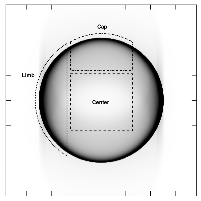
Figure 1.— Model and spectrum for $\phi=30^{\circ}$. Dashed line is the center region, dotted line is the limb regions and dot-dashed line is the cap regions. Solid line is the total of all regions.

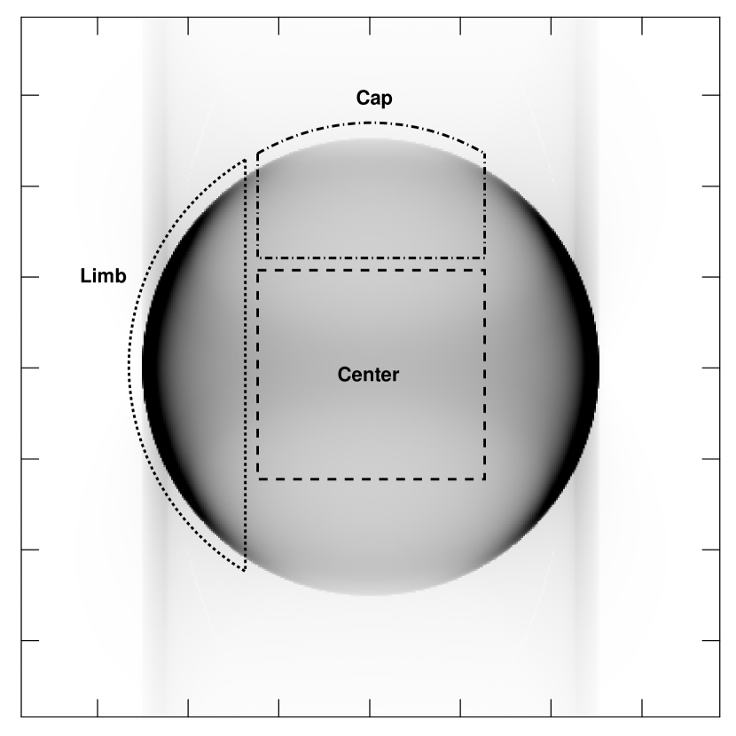
Figure 2.— Model and spectrum for for $\phi=60^{\circ}$. Dashed line is the center region, dotted line is the limb regions and dot-dashed line is the cap regions. Solid line is the total of all regions.

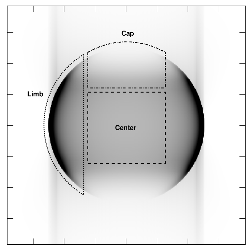
Figure 3.— Model and spectrum for for $\phi=90^{\circ}$. Dashed line is the center region, dotted line is the limb regions and dot-dashed line is the cap regions. Solid line is the total of all regions.

The submodel spectra are plotted in Figures 1-3, for three values of the aspect angle $\phi$ between $B_{1}$ and the line of sight. The integrated spectrum is insensitive to $\phi$, since at these frequencies the emission is extremely optically thin, but the submodels differ since the flux is apportioned differently among the regions as a function of $\phi$. For instance, the distinction between “cap” and “limb” begins to vanish as $\phi$ decreases; at $\phi=0$ (not shown), the image would be circularly symmetric on the sky (though our definitions of cap and limb encompass different fractions of the image area). These are spectra for a set of parameters $B_{1}$, etc., whose values are arbitrary, for the purpose of comparison among subregions. For all values of $\phi$, we notice that even though the limb regions cover the smallest area, the limbs still make the largest contributions to the total. At low enough frequencies where the curvature has not yet become important, the limb flux is about half the total for all values of $\phi$, while the center contribution to the total drops from 0.32 to 0.19 (as $\phi$ drops from $90^{\circ}$) and the cap rises from 0.21 to 0.34.

The limb emission is dominated by lines of sight nearly tangent to the shell at the very edge, and as the frequency increases and the emission is restricted (by electron energy losses) to thinner and thinner postshock regions, those lines of sight shorten quickly, so that for larger values of $\phi$, the integrated limb spectrum falls off more quickly than that of the center, which for larger values of $\phi$ also includes the highest-energy electrons (found near the “equator”). The softest spectrum is that of the caps, which include regions where the obliquity $\theta_{\rm Bn}$ is always near 0 (parallel shocks); for low values of $\phi$, the center does not contain any of the “equator” regions so its spectrum is softer as well. All these differences in the rolloff frequencies (the frequency where the decrement from a power law is approximately a factor of 6) amount to no more than 50% of the input model value of $\nu_{\rm rolloff}$ because of the relatively steep dropoff of the spectrum.

Anticipating the application of these models to SN 1006, we note that few objects are likely to be so symmetric that all parts of these models will fit the respective regions of the remnants. In the SRCUT and spatially-integrated SRESC models already in XSPEC, the models are given as decrements below the extrapolation of the power-law from radio frequencies. The principal difference among the region submodels is in normalization; the amount of curvature difference is relatively small, largest at $\phi=90^{\circ}$ and decreasing as $\phi$ decreases.

Figure 4.— A comparison of a limb-brightened model (solid line) to actual NE-SW slices from the Parkes+Molonglo radio image (dash-dot) and the ASCA GIS image (dashes). Note that there is not enough central flux in either the X-ray or radio image for the morphology of SN 1006 to be explained entirely by limb brightening.

In applying these models to SN 1006, we are forced to confront a significant problem: as demonstrated in Figure 4 at both radio and X-ray wavelengths the model overpredicts the emission from the center of SN 1006. We will discuss SN 1006’s lack of symmetry briefly in Section 7.4. However, we do not attempt to model the detailed radio emission in this paper. We can model X-ray emission without presuming a radio structure by using the observed radio fluxes and decrements in our XSPEC models. That is, we measure the dropoff in the X-ray spectrum from the observed, not the theoretical, radio fluxes.

Similarly, we assume that the same value of $\lambda_{\rm max}$ characterizes the emission in all regions. If that is not the case, one should in principle produce a totally new theoretical model incorporating some assumed spatial variation of $\lambda_{\rm max}$. However, given the relatively small variations in curvature for different regions, we shall adopt a more phenomenological approach, and allow the fitted rolloff frequencies in the different regions to vary if necessary.

We shall proceed under the assumption that the bilateral symmetry of SN 1006 is due to an ambient magnetic field close to the plane of the sky, that is, $\phi\cong 90^{\circ}$. The differences of model curvatures with obliquity in the ASCA band are small enough that this should not be a restrictive assumption. In general, substantially longer integration times would be necessary for current X-ray satellites to detect these subtle differences in curvature.

3.2. Thermal model

Since our primary interest is in the nonthermal emission, we fit thermal emission from the remnant with the simplest reasonable model VPSHOCK. Wherever we specify that a thermal model was used, we mean VPSHOCK. This is a plane-parallel shock model with variable abundances (Borkowski, Lyerly, & Reynolds, 2001). It represents an improvement over single-temperature, single-ionization timescale, non-equilibrium ionization models by allowing a distribution of ionization timescales. In principle one might expect improvements in the results of thermal modeling through the use of models at the next level of sophistication, such as Sedov or multitemperature models. However, it is already clear from high quality XMM-Newton and Chandra observations that thermal spectra demand an even higher level of modeling. A promising method is demonstrated in Badenes et al. (2003) where one-dimensional simulations of different types of explosions are used to generate synthetic spectra which are then compared to X-ray observations of Tycho. We will limit ourselves to the simplest reasonable thermal models, which here play a subordinate role to the nonthermal models.

4. X-ray observations

Unless stated otherwise SIS 0 & 1 datasets from the same observation were fit for each region. Full descriptions of the datasets used are given in Table LABEL:data6. We used SIS BRIGHT data at high and medium bit rate. The standard REV2 screening was used, and data were grouped with minimum of 20 counts per channel for valid $\chi^{2}$ analysis. The background spectra were obtained from the 1994 Blank Sky event files in the case of PV 4-chip observations and from off source areas for AO4 2-chip observations. We compared the results of subtracting the two types of backgrounds and found the differences in the resulting data were minor. What was not minor were gain shifts between GIS and SIS data. We intended to fit GIS and SIS data simultaneously to obtain better statistics. However, we found significant line shifts between the GIS and SIS. The difference was 70-80 eV in strong line energies (silicon is prominent). Experimental GIS matrices reduced the shift in Si line energy by $\sim$20 eV, but they were unable to completely remove the shift. We therefore chose the SIS instrument over the GIS for energy reliability and higher spatial and spectral resolution.

Spectra from the GIS do have one advantage over the SIS spectra. The GIS detectors have a higher effective area at high energy – since this extra signal to noise could have implications for the regions dominated by nonthermal emission we verified the results obtained from the SIS spectra by checking elliptical GIS regions in the NE and southwest (SW). The energy shifts between GIS and SIS are less important for measuring the continuum. The GIS 2 and GIS 3 data were jointly fit for each limb. We obtained radio fluxes (norm) from the same regions used to extract X-ray counts, and obtained background from regions of similar size outside each respective limb. We discuss the results of this comparison at the end of Section 6.1.

5. Radio observations

In Paper I, since the entire remnant was being fit, we obtained the normalization for the synchrotron models from single dish flux measurements. However, in order to separate limb from center emission we now needed accurate spatially resolved fluxes. Interferometric images have the fundamental problem that zero-spacing flux (the total flux in the image) is not measured. It is well known that maps without this “zero-spacing information” are missing the information needed to accurately reconstruct the total flux (Holdaway, 1999). The absence of short interferometric spacings showed up prominently for SN 1006 as negative flux densities in the center, NW, and SE regions in the images published in Reynolds & Gilmore (1986, 1993) and Moffett, Goss & Reynolds (1993). “Zero-spacing information” can only be restored to interferometric maps by adding single dish observations. Therefore we obtained an 843 MHz map created with data from both the Molonglo Observatory Synthesis Telescope (MOST), an East-West parabolic interferometer with UV coverage from 15 meters to 1.6 kilometers, and the Parkes 64-meter radio telescope, resulting in an image with resolution of $44^{\prime\prime}\times 66^{\prime\prime}$ (Roger et al., 1988). The total flux in the Roger et al. image agrees with single dish measurements and in this map no regions of the SNR have negative fluxes.

We measured the radio flux in the exact regions from which we extracted spectra by using a region file in sky coordinates to extract both the spectrum and an X-ray image. That image was loaded into AIPS, convolved to a resolution of 11″ to smooth the X-ray sampling, and aligned to the radio image with AIPS task HGEOM. The radio image was then clipped everywhere the X-ray image was blank, and the remaining flux was measured at the observing frequency (0.834 GHz) and then extrapolated to 1 GHz according to the single dish spectral index of 0.6 (Green, 2001).

6. Fits to data

We have fit and plotted the ASCA data from 0.4-10.0 keV. While 0.4 keV is below where ASCA data are normally considered reliable (generally above 0.6 keV and for the most recent data, only above 1.0 keV) we have chosen to use these data for several reasons. First, most of the datasets used are from the early performance verification phase (PV), prior to significant chip damage. Second, SIS0 and SIS1 are still in good agreement in that region – one test for data reliability. Finally, there were additional problems fitting regions from the center, southeast (SE) and northwest (NW) in the vicinity of 0.6 keV. Without including data from 0.4-0.6 keV, XSPEC was free to fit models with extremely high flux at low energies. While we do not trust the data sufficiently to report abundances measured at low energies, we believe the data can be trusted to rule out fluxes high by a factor of two or more. Finally, the lowest energies in each fit were dominated by thermal emission. As stated above, the main purpose of this work was to test models against nonthermal emission, which dominates at higher energies.

There were slight variations reported by SIS0 and SIS1 in the measured flux. While $\chi^{2}_{\nu}$ could be slightly improved by allowing the normalizations of the models in the two detectors to vary slightly, we did not choose to do so, preferring a slightly higher $\chi^{2}_{\nu}$ over introducing further uncertainties in norm.

We began by fitting solar-abundance thermal models (PSHOCK) to each of the regions (with a limb model in the NE and SW). These models fit very poorly, with $\chi^{2}_{\nu}$ ranging from 3.6-20 and obvious line residuals. We can say with certainty that even in the bright limbs where the nonthermal emission dominates, SN 1006 is not well described by solar abundance models. Henceforth, as we discuss our fits, all the VPSHOCK models we employ allow the individual abundances to vary.

Table LABEL:everything contains the results of the fits to each region of the remnant, for each model combination as described below. Included are $\chi^{2}$ and the number of degrees of freedom (DOF, column 1). The following two columns determine the nonthermal model: the 1 GHz norm (the flux in Jy, measured from the radio map) in column 3 (difference between SIS 0 and SIS 1 are a result of gap location, rather than chip differences), and in column 4, the $\nu_{\rm rolloff}$ ($\nu_{\rm rolloff}$ in Hz for all SRESC submodels). Thermal parameters from the VPSHOCK model include: the temperature found by each thermal model in units of keV (column 5) and the ionization timescale $\tau\equiv n_{e}t$ in units of s cm^-3 (column 6). In column 7 we give the emission measure (norm), defined as $\text@frac{10^{-14}}{4\pi D^{2}}\int n_{e}n_{H}dV$ where $D$ is the distance to the source in centimeters. The fitted abundances are listed in column 8-12, given as $\text@frac{<X/X_{\sun}>}{<Si/Si_{\sun}>}$ (by number, not mass, from Grevesse & Anders, 1989). Since the hydrogen abundance is poorly constrained by the fits, abundances were fit relative to silicon. Errors given in Table LABEL:everything are 1.5$\sigma$ errors (87% confidence interval). As in Paper I, for both GIS and SIS data, we assumed an absorption column density of 5$\times 10^{20}$ cm^-2, using the Wisconsin absorption model, wabs.

Note that, except where specified, all synchrotron models were fit with normalization and spectral index fixed, as measured from radio observations. There is considerable degeneracy in the model between norm, $\alpha$, and $\nu_{\rm rolloff}$, as demonstrated in Table LABEL:limits, but radio measurements allow us to input, rather than fit, norm & $\alpha$.

6.1. Brighter limbs: northeast and southwest

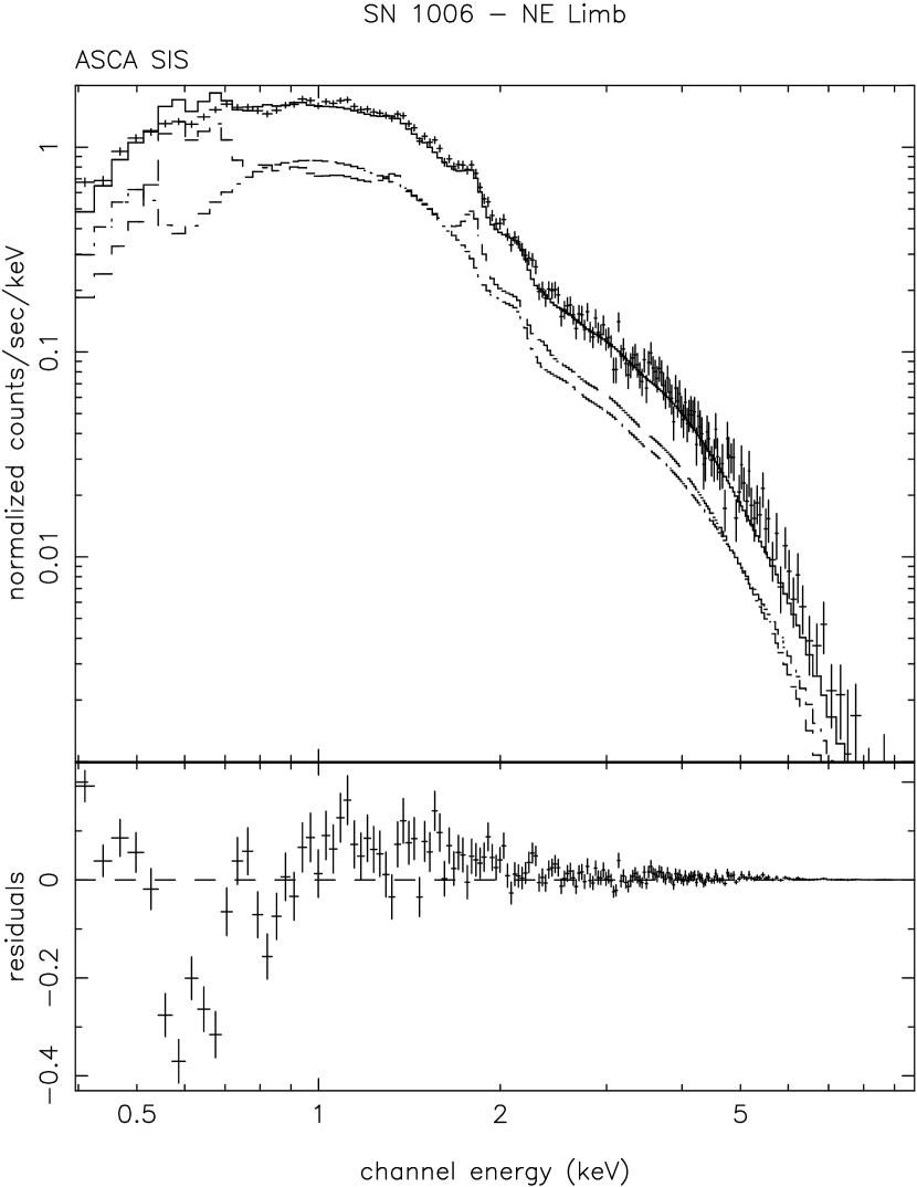
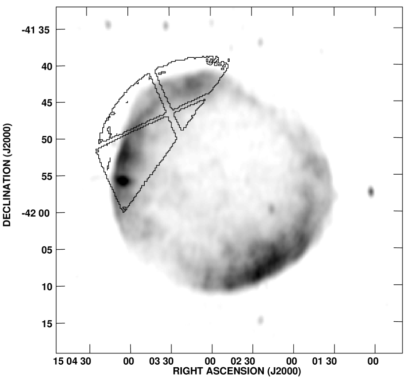
Figure 5.— Thermal and nonthermal fits to the northeast limb.

Figure 6.— Thermal and nonthermal fits to the southwest limb.

We began by searching for firm upper bounds to the synchrotron emission from the bright limb regions, shown in Figures 5 & 6. We did this by finding the maximum amount of the limb model tolerated by the SIS NE and SW regions, assuming a spectral index of 0.60 and limb norm measured from the radio, i.e. we raised $\nu_{\rm rolloff}$ until it threatened to exceed the data at high energies. We found that the spectra of the NE and SW regions are not identical (see Figure 7). The NE could tolerate a maximum $\nu_{\rm rolloff}$ of 7$\times 10^{17}$ Hz while the SW could only tolerate a maximum $\nu_{\rm rolloff}$ of 4$\times 10^{17}$ Hz.

Figure 7.— The northeast and southwest limbs with the maximum amount of nonthermal synchrotron plotted.

We then fit the data with combined thermal and nonthermal models, using VPSHOCK (variable abundances)+limb, shown in Figure 5. The results for the fit are given in Table LABEL:everything, row 1. The combined thermal and nonthermal fit achieved a $\chi^{2}_{\nu}$$\sim$1.8. Residuals from the fits primarily show discrepancies between SIS0 and SIS1 between 0.5 and 1.0 keV.

With the addition of a thermal model the $\nu_{\rm rolloff}$ for the NE dropped to 3.3$\times 10^{17}$ Hz with 1.5$\sigma$ limits of 2.6$\times 10^{17}$ and 3.8$\times 10^{17}$ Hz. The SW had a $\nu_{\rm rolloff}$ of 2.3$\times 10^{17}$ Hz with 1.5$\sigma$ limits of 1.9$\times 10^{17}$ and 2.6$\times 10^{17}$ Hz. These fitted values of $\nu_{\rm rolloff}$ do appear significantly different, though not by as much as the maximum values above. This agrees with the higher radio-to-X-ray ratio in the SE shown in Figure 4. In order for the radio-to-X-ray ratio to be lower than in the NE, $\nu_{\rm rolloff}$ must be lower (since $\alpha$ is fixed.) The thermal component of the NE had a temperature of 1.85${}_{1.81}^{1.89}$ keV and ionization timescale of 5.2${}^{6.8}_{3.8}\times 10^{9}$ s cm^-3. The total flux from 0.4 to 10.0 keV in the NE was 6.1$\times 10^{-11}$ ergs cm^-2 s^-1, of which 47% was from the synchrotron model. The SW had a temperature of 1.87${}_{1.79}^{1.89}$ keV and an ionization timescale of 1.5${}_{1.4}^{1.7}\times 10^{10}$cm^-3 s. The total flux in the SW was 4.3$\times 10^{-11}$ ergs cm^-2 s^-1, of which 46% was from the synchrotron model.

The GIS data, in contrast to the SIS data, show no obvious lines between 2 and 10 keV. Therefore there is little purchase for a thermal+nonthermal fit, although for comparison with SIS results we did try fits with SRESC and SRESC+VPSHOCK models. Since the GIS has a much wider bandpass than the SIS we also allowed the spectral index to vary, in order to eliminate the possibility that freezing $\alpha$ within the narrower SIS bandpass could introduce false results in $\nu_{\rm rolloff}$ (as discussed above and shown in Table LABEL:limits the degeneracy in norm, $\nu_{\rm rolloff}$, and $\alpha$ decreases the usefulness of fitting $\alpha$).

The 1 GHz norms from the GIS regions were 3.37 Jy for the NE and 5.11 Jy for the SW. (All errors on GIS observations are 1.65 $\sigma$, i.e. 90% confidence interval.) With $\alpha$ fixed to 0.6, we obtained values of $\nu_{\rm rolloff}$ of $5.89_{5.79}^{5.99}\times 10^{17}$ Hz in the NE and $\nu_{\rm rolloff}=3.25_{3.19}^{3.30}\times 10^{17}$ Hz in the SW.  With $\alpha$ allowed to vary we obtained $\nu_{\rm rolloff}=2.61_{2.19}^{2.95}\times 10^{17}$ Hz and $\alpha=0.55\pm 0.01$ in the NE, and $\nu_{\rm rolloff}=2.62_{2.25}^{3.12}\times 10^{17}$ Hz and $\alpha=0.59\pm 0.01$ in the SW. The thermal+nonthermal fits were carried out with SRESC plus a solar abundance VPSHOCK model. With $\alpha$ fixed at 0.6, we found $\nu_{\rm rolloff}$ to be $4.50_{3.57}^{5.11}\times 10^{17}$ Hz in the NE and $2.65_{1.95}^{3.08}\times 10^{17}$ Hz in the SW.

This confirms results found from the SIS fits, including the slightly higher rolloff frequency in the NE. In the thermal+nonthermal fits the GIS do not show any significant differences in $\nu_{\rm rolloff}$ that might be expected from the better GIS sensitivity at high energies. The results are consistent with the results for SIS fits, which are preferred since they more accurately constrain the thermal emission.

6.2. Fainter limbs: northwest and southeast

6.2.1 Northwest

Our initial assumption in applying the simple escape model was that all regions of the remnant would be fit with varying amounts of norm, measured in radio observations, but the same spectral index and $\nu_{\rm rolloff}$. We note that this procedure normalizes away any departure of the radio morphology from model predictions (for example, the simple SRESC model predicts higher brightness in the remnant center than is observed). It simply requires that no additional departures from model predictions would be necessary between radio and X-ray wavelengths.

However, it is immediately clear that while the NE and SW regions have similar $\nu_{\rm rolloff}$’s (average 2.8$\times 10^{17}$ Hz), that this value of $\nu_{\rm rolloff}$ in the cap submodel, with norm appropriate to the NW and SE, clearly contradicts the NW and SE data, even before addition of a thermal model required by the presence of lines (see Figures 8b and 9b). This agrees with the high spatial resolution XMM-Newton results of Decourchelle (2002) which found $\nu_{\rm rolloff}$ varying with both radius and azimuth.

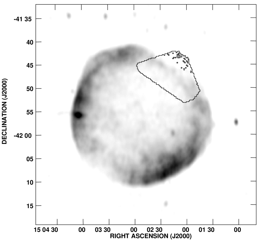
Figure 8.— Northwest: a) SIS region shown on the Parkes radio image b) high cap model with $\nu_{\rm rolloff}$ measured at the limbs c) thermal model VPSHOCK.

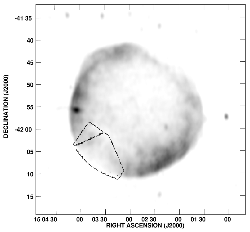
Figure 9.— Southeast: a) SIS region shown on the Parkes radio image b) cap model emission predicted by the $\nu_{\rm rolloff}$ measured at the limbs c) thermal model VPSHOCK.

Fits to the NW region with a thermal-only variable abundance model (shown in Figure 8c) yielded a $\chi^{2}_{\nu}$ of 1.80. Deficiencies in the thermal model can be noted in residuals near 0.7 and 0.9 keV (Fe L-shell or Ne K$\alpha$). Full results are given in Table LABEL:everything, row 5. The temperature given by the fit was 1.2${}^{1.3}_{1.0}$ keV and $\tau=6.5^{7.9}_{5.5}\times 10^{9}$ cm^-3 s. The total flux from this fit was 1.3$\times 10^{-11}$ ergs cm^-2 s^-1. While a fit with thermal+nonthermal models was attempted the data preferred no nonthermal component.

It was critical to place upper limits on the amount of nonthermal emission even in regions where no nonthermal component was required so we used the following procedure: we added a nonthermal model (beginning with $\alpha=0.60$, $\nu_{\rm rolloff}$=2.8$\times 10^{17}$ Hz and norms measured from the radio image) to the best thermal-only fit (given in Table LABEL:everything, row 5) and then changed each of the three nonthermal parameters in turn ($\alpha$, $\nu_{\rm rolloff}$, and norm), holding the others fixed until the $\chi^{2}$ rose by $\sim$2.3, a 1.5$\sigma$ change. The results of these fits are given in Table LABEL:limits with the varying quantity in bold face. With this method we found that for the NW data the cap model had a maximum $\nu_{\rm rolloff}$ of 1.1$\times 10^{17}$ Hz, or a maximum norm of 0.25 Jy at 1 GHz, or a spectral index $\alpha$ of 0.67 or steeper. This places a limit of $\leq$8% on the nonthermal contribution to the NW flux.

6.2.2 Southeast

As with the NW, using the value of $\nu_{\rm rolloff}$ measured in the NE and SW regions overpredicted the observed flux in the SE (see Figure 9b). Thermal fits with variable abundances to the SE (see Figure 9d) were significantly worse than the NW. $\chi^{2}_{\nu}$ was $\sim$3 for a single VPSHOCK model, a two-VPSHOCK model (not shown), and a cap+VPSHOCK model. Interestingly, despite a much worse $\chi^{2}_{\nu}$ the residuals look very similar to those in the NE – obvious line-like residuals at 0.7 and 0.9 keV.

The thermal-only model (Table LABEL:everything, row 7) had a temperature of 1.1${}^{1.2}_{1.0}$ keV and a $\tau=2.3^{2.8}_{1.8}\times 10^{10}$ cm^-3 s. As above for the NW, while a combined thermal and nonthermal model was tried, the data preferred no nonthermal component at all.

Following the method outlined above for the NW, we set limits on the nonthermal emission. In the SE we can exclude a $\nu_{\rm rolloff}$ above 1.1$\times 10^{17}$ Hz or a spectral index, $\alpha$ flatter than 0.67, or a norm above 0.2 Jy at 1 GHz. The total flux of this faint region is 8.6$\times 10^{-12}$ ergs cm^-2 s^-1 and the maximum nonthermal contribution is $\leq 9\%$.

6.3. Center

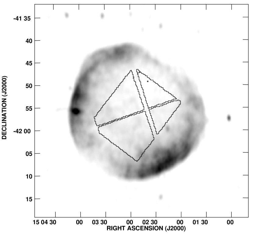
Figure 10.— Center: a) SIS region shown on the Parkes radio image b) center model emission predicted by the $\nu_{\rm rolloff}$ measured at the limbs c) thermal model VPSHOCK.

We turn now to the center of SN 1006. Unlike the NW and SE, the center data could just tolerate the nonthermal model center with fixed $\nu_{\rm rolloff}$, shown in Figure 10b. However, joint fits soon reduced the nonthermal component to $\leq$5% (using the method outlined in fits for the NW and SE). Both combined and thermal-only models had very high $\chi^{2}_{\nu}$($>5$). Thermal-only fits (Figure 10d and Table LABEL:everything, row 3) reported a temperature of 0.82${}^{0.85}_{0.76}$ keV and a $\tau=2.5^{2.8}_{2.3}\times 10^{10}$ cm^-3 s. As with the NW and SE, when a thermal+nonthermal model fit was attempted the data preferred no nonthermal component. All fits to the center show residuals similar to the NW and SE.

The thermal fits for each region of the SNR reveal elevated abundances. We can make a separate case for supersolar abundances by measuring the equivalent width of the well-separated Si K$\alpha$ line in the center where the lines are strongest. The result is an equivalent width for silicon of 600 $\pm$ 50 eV (1.65 $\sigma$, 90% confidence). We draw conclusions from this in Section 7.2.

7. Discussion

7.1. Difference between the NE and SW limbs

The NE and SW regions do have slightly different spectra, with values of $\nu_{\rm rolloff}$ differing by a significant amount in both SIS and GIS fits including a thermal component. (The $\nu_{\rm rolloff}$ values bracket the Paper I value averaged over the remnant of $3.1\times 10^{17}$ Hz.) This is not, however, sufficient to explain the differences in TeV detection of the NE and SW regions (assuming as in Paper I that the TeV detection is cosmic microwave background photons, inverse-Compton scattered by the same population of electrons that produce the X-ray synchrotron emission). The small difference in $\nu_{\rm rolloff}$ between NE and SW regions only produces a difference of 5% in this flux at 1 TeV. Even $\nu_{\rm rolloff}$’s differing by factor of three only produce a difference of $\sqrt{3}\sim 70$% in $E_{max}$. A difference in the spectral index is far more likely to produce the differences between synchrotron emission in the NE and SW regions which would be required to explain differences in $\gamma$-ray detection (although, as discussed below the spectral index cannot account for the entire change).

Using the formula given in §3.1 and assuming a magnetic compression ratio $r$=4 and value $B_{1}$= 3 $\mu G$ as found in Paper I, we find that the $\nu_{\rm rolloff}$ of 3.3${}^{3.8}_{2.6}\times 10^{17}$ Hz in the NE gives a $\lambda_{max}$=1.5${}^{1.6}_{1.3}\times 10^{17}$ cm and in the SW a $\nu_{\rm rolloff}$ of 2.3${}^{2.6}_{1.9}\times 10^{17}$ Hz gives $\lambda_{max}$=1.2${}^{1.1}_{1.3}\times 10^{17}$ cm. These values imply electron escape above 33 TeV in the NE or 28 TeV in the SW, similar to the value of 32 TeV quoted in Paper I, as is to be expected.

7.2. Thermal fits

As stated earlier, the focus of this work was on testing nonthermal models. Therefore only the simplest plane shock model was used to fit thermal emission. We ruled out solar-abundance thermal emission in each region of the SNR and then used the variable-abundance model, VPSHOCK, for the remainder of our fits.

The quality of the fits varied widely across the SNR. In bright regions such as the NE, the SW, and the NW, the fits gave marginal values of $\chi^{2}_{\nu}\sim 1.8$. Fainter regions such as the center and the SE were poorly fit by VPSHOCK with $\chi^{2}_{\nu}>5.0$. However, despite different values of $\chi^{2}_{\nu}$, the residuals of all regions with significant thermal emission (SE, NW and center) had line-like residuals at 0.7 and 0.9 keV. This casts suspicion on even the better fits and suggests problems with the underlying atomic data since this is where 3s to 2p transitions in Ne-like Fe ions are found. These transitions appear to be stronger than expected in astrophysical sources, including SNRs (as seen in van der Heyden et al., 2002).

In the current NEI v1.1 models in XSPEC which we use, Fe L-shell data are based on calculations by Liedahl, Osterheld, & Goldstein (1995) for electron collisional excitation of Ne- to Li-like Fe ions, and on older atomic data for inner-shell processes in Mg-like and Na-like Fe ions (Hamilton & Sarazin, 1984). Indirect processes such as inner-shell collisional ionization, radiative and dielectronic recombination, and resonance excitation are not included, although they have been shown to be important in enhancing 3s to 2p transitions in the Ne-like ion in particular (Gu, 2003). The enhancement of 3s to 2p transitions in the Ne-like ion due to the inner-shell ionization of the Na-like ion might be particularly important in high-temperature plasmas at low ionization ages, such as those encountered in SN 1006. In addition, Chen et al. (2003) showed recently that atomic resonances in the electron collisional excitation of Ne-like Fe are also important, although they have been neglected in the past. So there are many deficiencies in Fe L-shell atomic data which could result in poor fits in the 0.7-0.9 keV range.

We tested this hypothesis by adding lines arising from the inner-shell ionization of the Na-like Fe ion into XSPEC NEI v2.0 models. These models are based on the Astrophysical Plasma Emission Database (APED; Smith et al., 2001), and are currently missing several processes important in NEI conditions, but they allow for easy modification of the atomic database. We added three lines of the Ne-like ion at 17.098, 17.053, and 16.778 ${\rm\AA}$ (0.725, 0.727, and 0.739 keV, the strongest at 0.725 keV). For a shock model with parameters appropriate for the NW region of SN 1006 ($kT=1.17$ keV and $\tau=6.5\times 10^{9}{\rm cm}^{-3}$), their contribution to the Fe spectrum is substantial. So it appears certain that the current fits to SN 1006 spectra use inadequate Fe L-shell atomic data, and that one problem with current thermal fits can be traced to Fe L-shell data. In particular, missing lines from inner-shell ionization of Na-like Fe ions are certainly a problem for the NW, and most likely elsewhere. Since this paper is primarily concerned with the nonthermal emission and better spectral information (for smaller spatial scales) has been obtained by XMM-Newton and Chandra we defer advanced models to a future paper.

This may not be the only issue preventing us from finding adequate thermal fits. X-ray spectral modeling of Type Ia SNRs (Badenes et al., 2003) has revealed significant differences in physical conditions between chemically-distinct layers of shocked ejecta. In particular, the emission-measure averaged ionization timescale of Fe appears to be shorter than that of other abundant elements in most models considered by Badenes et al. (2003, Fig. 6). It is then unlikely that the chemically homogeneous VPSHOCK model can provide a satisfactory fit to both Fe L-shell lines and lines produced by other elements. Substantial improvements in both Fe L-shell atomic data and in spectral models are required in order to make further progress in modeling SN ejecta in SN 1006.

The Paper I fits to the total flux of SN 1006 achieved better values, $\chi^{2}_{\nu}$=1.2. However, the better fits are causes by two factors: the poorer spectral resolution of the ASCA GIS instrument and the fact that the integrated spectrum is dominated by the synchrotron contributions of the two bright limbs which are well described by our models.

One conclusion that can be drawn from the thermal fits in Table LABEL:everything is that while the thermal fits may be oversimplified, the VPSHOCK model is clearly sensitive to both thermal parameters and abundances. Whereas we might have expected large uncertainties, the 1.5$\sigma$ statistical errors are rarely more than 8%. Clearly, the data are capable of constraining thermal models; the correct thermal model should yield significant information.

While our thermal model fits to the center were of poor quality statistically, they strongly implied elevated abundances of heavy elements such as Si. Fortunately, a more model-independent criterion is available: the equivalent width of the Si K$\alpha$ complex (Si XIII). Our measured value of $600\pm 50$ eV is higher than a plane shock with solar abundances could achieve until $\tau\sim 3\times 10^{10}$ cm^-3 s, by which time the shock has $kT$ considerably above 1 keV, and should have much higher ratios of O VII to Si XIII than we observe (Long et al., 2003). We conclude that the central emission is dominated by shocked ejecta.

7.3. Nonthermal results

Our spatially resolved subsets of SRESC, cap, limb, and center, differ surprisingly little from one another or from the total (SRESC itself), though the differences we do see (§3.1) are in the sense one would expect. However, for these ASCA data, and in fact for most data from current X-ray telescopes, the differences between the spatially integrated SRESC model and the submodels are not likely to be distinguishable. This could not have been predicted in advance, but it is fortunate for data analysis. However, our conclusions about the lack of cylindrical symmetry are stronger for our having based them on the appropriate submodels that symmetry would require.

The most striking result from the spatially resolved fit is that the SRESC submodels with values of $\nu_{\rm rolloff}$ that fit the limbs, do not fit the spectrum in the center, NW and SE. There are several possible explanations, with interesting consequences. First, it is possible that the SRESC submodels are an accurate description of the nonthermal emission and that the value of $\nu_{\rm rolloff}$ differs from one region to the next. Since $\nu_{\rm rolloff}$ $\propto\lambda^{2}B^{3}$ a difference in $\nu_{\rm rolloff}$ would imply a change in the external magnetic field or the maximum wavelength of MHD waves available for scattering. The variation of the $\nu_{\rm rolloff}$ parameter across the remnant marks a significant departure from the simple assumptions of the escape model. We can offer no justification for this but if $B$ or $\lambda_{max}$ could be isolated they would be important probes for the shock physics.

As demonstrated in Table LABEL:limits, the SRESC submodels show some degeneracy between $\nu_{\rm rolloff}$ and the radio spectral index $\alpha,$ in that a given X-ray to radio flux ratio can be produced (within limits) by flatter spectra with lower $\nu_{\rm rolloff}$, or steeper spectra with higher $\nu_{\rm rolloff}$. A large source of error in all synchrotron fits is the uncertainty in $\alpha$. An uncertainty in $\alpha$ of $\pm$ 0.1 at 1 GHz can change the extrapolated flux in the 2 to 3 keV range by a factor of 7. In addition to being poorly measured by single dish radio observations, the spectral index could vary across the source. We can, however, rule out the possibility that spectral index is solely responsible for the variation in $\nu_{\rm rolloff}$. While radio observations cannot constrain $\alpha$ to better than $\pm$0.02, single-dish observations firmly exclude an $\alpha$ as steep as 0.67. Since the two limbs dominate the total radio emission as they do the X-ray emission, the kind of difference between limbs that would be required seems unlikely. We cannot, of course, rule out a contrived situation in which the spectrum of the SW suddenly steepens significantly compared to the NE at radio frequencies higher than have been measured. Nevertheless, the question of a varying spectral index across the remnant is intriguing. Many researchers have searched for variations in radio spectral index in SNRs as an indication of changes in shock acceleration. However, interferometric observations are ill suited to this kind of study (see discussion in Dyer & Reynolds, 1999) and current observations of SN 1006 can neither support nor contradict this premise.

A second possibility is that the physics in the synchrotron model that underlies SRESC and submodels is inadequate to describe the nonthermal emission. One critical assumption is that the diffusion coefficient $\kappa$ is proportional to the energy. A divergence from this assumption at the highest energies could have serious consequences.

7.4. Morphology

We began our investigation by assuming cylindrical symmetry about the NW-SE axis. We can now rule this out with a fair amount of certainty. If SN 1006 were cylindrically symmetric a line of sight through the center would sample a predictable amount of the nonthermal emission which brightens the limbs. This is ruled out by the fact that the SRESC submodels over-predict the high energy flux in the NW, SE and center, as demonstrated in Figures 8b, 9b and 10b. This deficit of central emission is in addition to the deficit already present between observed and theoretical radio images in the SRESC model, since we are using measured rather than theoretical values of norm. An explanation which might account for the weaker central emission in radio compared to the simple model (for instance a substantial radial component to the magnetic field) cannot explain the additional deficit in X-rays. Any explanation must impact the X-ray emission differently than the radio emission.

That SN 1006 is not simply limb brightened due to a NW-SE symmetry is an uncomfortable conclusion, since it implies a preferred orientation between SN 1006 and the observer, although there are other arguments for asymmetry from Willingale et al. (1996), based on ratios between the X-ray emission in limbs and center as observed by ROSAT, and arguments derived from the spectra of the Schweizer-Middleditch star (Hamilton et al., 1997).

This asymmetry could take several forms. It is possible, likely in fact, that the upstream magnetic field is not uniform. There is already evidence for asymmetry in the NW, where H$\alpha$ is strongest – presumably the ambient medium outside the NW is, for some reason, less ionized. This would have an impact on electron acceleration. This could affect $\lambda_{max}$ in particular.

It is possible, of course, that fundamental assumptions made in the SRESC model are incorrect. While the agreement of the model with the bright limbs argues that the basic picture of electron acceleration to a power-law with an exponential cutoff is sound, at least in those regions, it is possible that a completely different geometry holds, for instance, one in which the bright limbs are “caps” seen edge-on rather than brightened limbs of an equatorial “belt.” The symmetry axis would then run NE-SW, but would need to be nearly in the plane of the sky. The reasons that the polar caps are brighter in synchrotron radiation in such a picture would need to involve some superior feature of parallel shocks for electron injection or acceleration, or perhaps magnetic-field amplification as suggested by Bell & Lucek (2001). A fundamental defect of such a picture is that remnants for which the ambient magnetic field is closer to the line of sight should appear in radio synchrotron images as two maxima surrounded by a steep-spectrum halo, a morphology which is not seen in any Galactic remnant.

7.5. Comparison with Chandra Results

Chandra observed part of the NE limb in Cycle 1 and part of the NW limb in Cycle 2. The smaller field of view, and charge-transfer-inefficiency problems for the front-illuminated CCDs, restricted initial analysis to much smaller regions than those we analyzed here. However, the results (Long et al., 2003) are consistent with ours. In the NE, thin filaments appeared to have completely line-free spectra, and were well described by an SRESC model with $\alpha=0.54$ and $\nu_{\rm rolloff}$ of $6.9\times 10^{17}$ Hz. Since Chandra was able to isolate a region immediately behind the shock only a few tens of arcsec in size, it is to be expected that the hardest electron spectrum (highest $\nu_{\rm rolloff}$) would be found there. Our GIS value for $\nu_{\rm rolloff}$, with $\alpha$ allowed to float, is close to this value, although slightly lower because of dilution from thermal emission and nonthermal emission further downstream where adiabatic and radiative losses begin to soften the spectrum. A region several arcminutes behind the shock in the NE was shown to have substantial line emission, and was fairly well described by a VPSHOCK+SRESC model with $kT\sim 1.4$ keV, $\tau\sim 3\times 10^{9}$ cm^-3 s, and a $\nu_{\rm rolloff}$ of $(3-6)\times 10^{17}$ Hz. Elevated abundances of heavy elements (chiefly Si and Fe) were required. These results are similar to our inferences about the thermal component in the NE, though these of course apply to a much larger region than the Chandra results. In the NW, a VPSHOCK fit to a small region coincident with the H$\alpha$ optical filament gave $kT\sim 0.9$ keV, $\tau\sim 6\times 10^{9}$ cm^-3 s, and required no nonthermal component (though it could tolerate a weak one). These results are comparable to those we report here from a much larger region. The broad similarities between fitted values of small regions with Chandra data and larger averages with ASCA data give some confidence that the systematic residuals we observe that degrade the statistical quality of our fits are not spacecraft-dependent systematic effects. (Of course, they may be inherent in the models or atomic data, which were the same in the two analyses.) While Chandra observations did include regions closer to the center of SN 1006, those were on ACIS-I chips subject to charge-transfer-inefficiency problems, and the data have not yet been analyzed.

7.6. Effect on Paper I Results

These new investigations change few of the results in Paper I. It is clear that synchrotron emission from the limbs dominates the total fit: the value of $\nu_{\rm rolloff}$ in Paper I was $3.0_{2.8}^{3.1}\times 10^{17}$ Hz, while fits to the limbs individually found $3.3\times 10^{17}$ and $2.3\times 10^{17}$ Hz.

While in theory more precise values for the postshock magnetic field strength, the energy in relativistic electrons and the electron efficiency (9 $\mu G$, 7$\times$10⁴⁸ ergs and 5% in Paper I) could be obtained from limb-only fits, in fact these will change insignificantly considering other uncertainties.

8. Conclusions

8.1. Nonthermal Emission

1. From comparing the limb-to-center ratio in X-ray and radio wavelengths (Figure 4), we find that the morphology of SN 1006 is not solely due to limb brightening of a cylindrically symmetric source about a line parallel to the bright limbs. This has the inescapable consequence that the observer is now required to have a particular vantage point with respect to the SNR.

2. SRESC provides a useful framework to describe synchrotron emission in SNR blast waves. Spatially resolved subsets of the SRESC model, cap, limb, and center, differ surprisingly little from the spatially integrated model, with the greatest differences occurring when the upstream magnetic field is in the plane of the sky. The differences are unlikely to be detectable with the current generation of X-ray telescopes.

3. The limb model provides a good description of the limbs of SN 1006, but the cap and center region models overpredict nonthermal emission in other regions of the remnant if $\nu_{\rm rolloff}$ is assumed to be constant everywhere.

4. We do find differences in the nonthermal spectrum between the NE and SW, but they are not sufficient to explain why only the NE is detected in TeV $\gamma$-rays, assuming the $\gamma$-rays are produced by inverse-Compton upscattering of the cosmic microwave background photons.

The usefulness of limb, cap, and center models for other SNRs is not obvious. Most SNRs have more complex morphology than SN 1006, and few present regions clearly appropriate for a center or cap model. While the limb model may be appropriate for filamentary structure at the edge of other SNRs, its curvature differs only very slightly from the SRESC model. We recall that the model SRESC, and its derivatives have several assumptions that make them unsuitable for SNRs of unknown type – the models presume a Sedov-phase remnant encountering a uniform upstream medium with a constant magnetic field. SRCUT, as discussed in Reynolds & Keohane (1999), which describes synchrotron radiation with a minimum of assumptions, may be a better choice for SNRs about whose environment less is known.

8.2. Thermal Emission

1. We can rule out solar abundances in the thermal models in all regions of the SNR, including regions dominated by nonthermal emission.

2. Simple thermal models are incapable of describing the ASCA data adequately. We note that in much smaller regions of SN 1006, the analysis of Chandra data encountered similar problems (Long et al., 2003). We believe that this is mainly caused by deficient Fe L-shell atomic data, where many important processes (such as inner-shell ionization of the Na-like Fe ion) are currently not included in NEI spectral codes. It is also likely that the available spectral models are not adequate for modeling chemically-inhomogeneous SN ejecta. A full analysis of the combined thermal and nonthermal emission from SN 1006 will require XMM-Newton and Chandra quality data with substantial improvements in atomic data and modeling.

3. To the extent that our thermal results can be trusted, we see elevated abundances which suggest the thermal emission contains substantial contributions from the reverse shock. Here the models agree with the silicon equivalent width, and with the results of other X-ray analyses of SN 1006.

Figure 11.—

Figure 12.—

Figure 13.—

References

- Allen, Gotthelf & Petre (1999) Allen, G.E., Gotthelf, E.V. & Petre, R. 1999, Proceedings of the 26th International Cosmic Ray Conference, astro-ph/9908209
- Badenes et al. (2003) Badenes, C., Bravo, E., Borkowski, K. J., & Domínguez, I. 2003, ApJ, 593, 358
- Bamba et al. (2003) Bamba, A., Yamazaki, R., Ueno, M., & Koyama, K. 2003, ApJ, 589, 827
- Bell & Lucek (2001) Bell, A. R. & Lucek, S. G. 2001, MNRAS, 321, 433
- Berezhko, Ksenofontov, & Völk (2002) Berezhko, E. G., Ksenofontov, L. T., & Völk, H. J. 2002, A&A, 395, 943
- Borkowski, Lyerly, & Reynolds (2001) Borkowski, K. J., Lyerly, W. J., & Reynolds, S. P. 2001, ApJ, 548, 820
- Chen et al. (2003) Chen, G.-X., Pradhan, A.K., & Eissner, W. 2003, J. Phys. B: At. Mol. Opt. Phys. 36, 453
- Decourchelle (2002) Decourchelle A. Proceedings from the symposium “New Visions of the X-ray Universe in the XMM-Newton and Chandra Era”, November 26-30, 2001, ESA SP-488 editor F. Jansen.
- Dyer et al. (2000) Dyer, K. K., Reynolds, S. P., Borkowski, K. J., Allen, G. E., & Petre, R. 2001, ApJ, 551, 439
- Dyer & Reynolds (1999) Dyer, K. K. & Reynolds, S. P. 1999, ApJ, 526, 365
- Green (2001) Green D.A., 2001, ‘A Catalogue of Galactic Supernova Remnants (2001 December version)’, Mullard Radio Astronomy Observatory, Cavendish Laboratory, Cambridge, United Kingdom (available on the World-Wide-Web at ”http://www.mrao.cam.ac.uk/surveys/snrs/”)
- Grevesse & Anders (1989) Grevesse, N. & Anders, E. 1989, American Institute of Physics Conference Series, 183, 1
- Gu (2003) Gu, M. F. 2003, ApJ, 582, 1241
- Hamilton & Sarazin (1984) Hamilton, A. J. S. & Sarazin, C. L. 1984, ApJ, 284, 601
- Hamilton et al. (1997) Hamilton, A. J. S., Fesen, R. A., Wu, C. -., Crenshaw, D. M., & Sarazin, C. L. 1997, ApJ, 481, 838
- Hendrick & Reynolds (2001) Hendrick, S. P. & Reynolds, S. P. 2001, ApJ, 559, 903
- van der Heyden et al. (2002) van der Heyden, K. J., Behar, E., Vink, J., Rasmussen, A. P., Kaastra, J. S., Bleeker, J. A. M., Kahn, S. M., & Mewe, R. 2002, A&A, 392, 955
- Holdaway (1999) Holdaway, M.A. 1999, ASP Conference Series v. 180, Synthesis Imaging in Radio Astronomy II (Editors. G.B. Taylor, C.L. Carilli, & R.A. Perley) ASP San Francisco, 401-418
- Hwang et al. (2002) Hwang, U., Decourchelle, A., Holt, S. S., & Petre, R. 2002, ApJ, 581, 1101
- Koyama et al. (1995) Koyama, K., Petre, R., Gotthelf, E. V., Hwang, U., Matsura, M., Ozaki, M., Holt, & S. S. 1995, Nature 378, 255
- Liedahl, Osterheld, & Goldstein (1995) Liedahl, D. A., Osterheld, A. L., & Goldstein, W. H. 1995, ApJ, 438, L115
- Long et al. (2003) Long, K.S., Reynolds, S.P., Raymond, J.C., Winkler, P.F., Dyer, K.K., & Petre, R. 2003, ApJ, 586, 1162
- Moffett, Goss & Reynolds (1993) Moffett, D.A., Goss, W.M., & Reynolds, S.P. 1993, AJ, 106 1566
- Reynolds (1996) Reynolds, S. P. 1996, ApJ, 459,L13
- Reynolds (1998) Reynolds, S. P. 1998, ApJ, 493, 375
- Reynolds & Gilmore (1986) Reynolds, S. P. & Gilmore, D. M. 1986, AJ, 92, 1138
- Reynolds & Gilmore (1993) Reynolds, S. P. & Gilmore, D. M. 1993, AJ, 106, 272
- Reynolds & Keohane (1999) Reynolds, S. P. & Keohane, J. W. 1999, ApJ, 525, 368
- Rho et al. (2003) Rho, J., Dyer, K.K., Borkowski, K.J., & Reynolds, S.P. 2003, ApJ, 581, 1116
- Roger et al. (1988) Roger, R. S., Milne, D. K., Kesteven, M. J., Wellington, K. J., & Haynes, R. F. 1988, ApJ, 332, 940
- Slane et al. (1999) Slane, P., Gaensler, B. M., Dame, T. M., Hughes, J. P., Plucinsky, P. P., & Green, A. 1999, ApJ, 525, 357
- Slane et al. (2001) Slane, P., Hughes, J. P., Edgar, R. J., Plucinsky, P. P., Miyata, E., Tsunemi, H., & Aschenbach, B. 2001, ApJ, 548, 814
- Smith et al. (2001) Smith, R. K., Brickhouse, N. S., Liedahl, D. A., & Raymond, J. C. 2001, ApJ, 556, L91
- Tanimori et al. (1998) Tanimori, T., et al. 1998, ApJ, 497, L25
- Tanimori et al. (2001) Tanimori, T., Naito, T., Yoshida, T., CANGAROO collaboration 2001, Proc. 27th ICRC (Hamburg, August 7-15, 2001)
- Uchiyama, Aharonian, & Takahashi (2003) Uchiyama, Y., Aharonian, F. A., & Takahashi, T. 2003, A&A, 400, 567
- Ueno et al. (2003) Ueno, M., Bamba, A., Koyama, K., & Ebisawa, K. 2003, ApJ, 588, 338
- Vink et al. (2000) Vink,J., Kaastra, J. S., Bleeker, J. A. M., & Preite-Martinez, A. 2000, A&A, 354, 931
- Vink & Laming (2003) Vink, J., & Laming, J.M. 2003, ApJ, 584, 758
- Willingale et al. (1996) Willingale, R., West, R. G., Pye, J. P. & Stewart, G. C. 1996,MNRAS, 278, 749