Covariant Magnetoionic Theory II: Radiative Transfer

Abstract

Accretion onto compact objects plays a central role in high energy astrophysics. In these environments, both general relativistic and plasma effects may have significant impacts upon the spectral and polarimetric properties of the accretion flow. In paper I we presented a fully general relativistic magnetoionic theory, capable of tracing rays in the geometric optics approximation through a magnetised plasma in the vicinity of a compact object. In this paper we discuss how to perform polarised radiative transfer along these rays. In addition we apply the formalism to a barotropic thick disk model, appropriate for low luminosity active galactic nuclei. We find that it is possible to generate large fractional polarisations over the innermost portions of the accretion flow, even when the emission mechanism is unpolarised. This has implications for accreting systems ranging from pulsars and X-ray binaries to AGN.

1 Introduction

The spectral and polarimetric properties of astrophysical objects can provide significant insights into their structure and dynamics. As a result, a number of theoretical investigations into the source of these properties have been undertaken. Many of these have been primarily concerned with the spectral properties alone, typically comparing a physically motivated accretion flow to observations. However, with the measurement of polarisation in a number of sources, a significant fraction of the focus has been turned towards reproducing their polarimetric properties. In the context of an accreting compact object, both general relativistic and plasma effects can play a role in determining these properties. In Broderick & Blandford, 2003 (hereafter Paper I) we demonstrated how to construct ray trajectories, in the geometric optics approximation, in a magnetoactive plasma in a relativistic environment. In order to apply this to realistic accretion environments it is necessary to be able to perform radiative transfer along these rays.

Non-refractive, polarised radiative transfer through magnetised plasmas is flat space has been extensively studied. A number of examples involving weak magnetic fields exist in the literature (see e.g. Sazonov & Tsytovich, 1968; Sazonov, 1969; Jones & O’Dell, 1977a, b; Ginzburg, 1970). More recently, investigations into the net effects of tangled magnetic fields (expected to be typical in magnetised accretion flows) have begun (see e.g. Ruszkowski & Begelman, 2002). However, none of these deal with general relativistic environments.

The importance of refraction in the propagation of radio wavelengths has long been appreciated in the context of the ionosphere (see e.g. Budden, 1964; Ginzburg, 1970). More recently, refraction has been studied in conjunction with pulsars (see e.g. Weltevrede et al., 2003; Petrova, 2002, 2000; Barnard & Arons, 1986; Arons & Barnard, 1986). Nonetheless, in all of these cases, the emission was assumed to originate from a region distinct from where the refraction occurred. Refractive lensing of neutron stars was considered by Shaviv et al., 1999, but ignored general relativisitic effects.

General relativistic studies into the propagation of polarisation in vacuum have been done. These have been primarily interested in the geometrical effects due to the parallel transport of the linear polarisation (see e.g. Agol, 1997; Laor et al., 1990; Connors et al., 1980). Alternatively, in Bromley et al., 2001, polarised emission in a general relativistic environment is considered. However, none of the typical plasma transfer effects (e.g. Faraday rotation) were included in these calculations. In Heyl et al., 2003, the vacuum birefringence due to strong magnetic fields was considered in the context of neutron star atmospheres. However, in both, refraction was completely ignored. There have been some attempts to study the problem of ray propagation in a covariant form (see e.g. Broderick & Blandford, 2003; Melrose & Gedalin, 2001), but in these the radiative transfer was not addressed.

As discussed in Paper I, refraction coupled with the presence of a horizon can be a source of significant polarisation when the observation frequency is near the plasma and cyclotron frequencies of emitting region. The sense of the resulting net polarisation is determined by the plasma parameters at the surface at which the polarisation freezes out (when the modes cease to be adiabatic and must be treated as if they were in vacuum). Typically, this will result in a net circular polarisation. In a future paper we will discuss astrophysical environments in which this may be the case, including applications to Sgr A^∗and high mass X-ray binaries.

We present a method for performing polarised radiative transfer through a strongly refractive magnetised plasma in a general relativistic environment. Additionally, we apply this to a model of a thick accretion disk. This is done in six sections with §2 briefly reviewing the formalism presented in Paper I, §3 discussing how to perform the radiative transfer in a magnetised plasma, §4 presenting low harmonic synchrotron as a possible emission mechanism, §5 presenting some results, and §6 containing conclusions. The details of constructing a magnetised, thick, barotropic disk are presented in the appendix.

2 Ray Propagation

While astrophysical plasmas will, in general, be hot, the cold case provides an instructive setting in which to demonstrate the types of effects that may be present. As a result, it will be assumed that the plasma through which the rays propagate will be cold, with a small component of emitting hot electrons. As shown in Paper I, the rays may be explicitly constructed given a dispersion relation, $D\left(k_{\mu},x^{\mu}\right)$ (a function of the wave four-vector and position which vanishes along the ray), by integrating the ray equations:

$$\frac{dx^{\mu}}{d\tau}=\left(\frac{\partial D}{\partial k_{\mu}}\right)_{x^{\mu}}\;\;\mbox{and}\;\;\;\frac{dk_{\mu}}{d\tau}=-\left(\frac{\partial D}{\partial x^{\mu}}\right)_{k_{\mu}}\,,$$ (1)

where $\tau$ is an affine parameter along the ray. Expanding Maxwell’s equations in the geometric optics limit provides the polarisation eigenmodes and the dispersion relation (given a conductivity):

$$\left(k^{\alpha}k_{\alpha}\delta^{\mu}_{\nu}-k^{\mu}k_{\nu}-4\pi i\omega\sigma^{\mu}_{~{}\nu}\right)E^{\nu}=0\,,$$ (2)

where $E^{\mu}$ is the four-vector coincident with the electric field in the locally flat, comoving rest frame (LFCR frame), $\omega\equiv-\overline{u}^{\mu}k_{\mu}$ ($\overline{u}^{\mu}$ is the plasma four-velocity which defines the LFCR frame), and $\sigma^{\mu}_{~{}\nu}$ is the covariant extension of the the conductivity tensor. For the cold, magnetoactive, electron-ion plasma (in the limit of infinite ion mass), the dispersion relation is

$$D\left(k_{\mu},x^{\mu}\right)=\\ k^{\mu}k_{\mu}-\delta\omega^{2}-\frac{\delta}{2\left(1+\delta\right)}\Biggl{\{}\Biggl{[}\left(\frac{e{\cal B}^{\mu}k_{\mu}}{m\omega}\right)^{2}-\left(1+2\delta\right)\omega_{B}^{2}\Biggr{]}\\ \pm\sqrt{\left(\frac{e{\cal B}^{\mu}k_{\mu}}{m\omega}\right)^{4}+2\left(2\omega^{2}-\omega_{B}^{2}-\omega_{P}^{2}\right)\left(\frac{e{\cal B}^{\mu}k_{\mu}}{m\omega}\right)^{2}+\omega_{B}^{4}}\Biggr{\}}\,,$$ (3)

where ${\cal B}^{\mu}$ is the four-vector coincident with external magnetic field in the LFCR frame, $\omega_{P}$ is the plasma frequency in the LFCR frame, $\omega_{B}$ is the cyclotron frequency associated with ${\cal B}^{\mu}$, and $\delta\equiv\omega_{P}^{2}/(\omega_{B}^{2}-\omega_{P}^{2})$, This is a covariant form of the Appleton-Hartree dispersion relation (see e.g. Boyd & Sanderson, 1969).

In general, the electromagnetic polarisation eigenmodes will not follow the same trajectories, and in particular will not follow null geodesics. As a result, the different polarisation eigenmodes will sample different portions of the accretion flow. As shown in Paper I, it is possible for one mode to be captured by the central black hole while the other escapes, leading to a net polarisation.

3 Polarised Radiative Transfer in Refractive Plasmas

Both emission and absorption are local processes. However, because the transfer of radiation necessarily involves a comparison between the state of the radiation at different points in space, global propagation effects need to be accounted for. These take two general forms: correcting for the gravitational redshift; and keeping track of the local coordinate system, i.e. ensuring that polarised emission is being added appropriately in the presence of a rotation of the coordinate system propagated along the ray. In addition, for a magnetoactive plasma, it is necessary to determine how to perform the radiative transfer in the presence of refraction.

3.1 Length Scales and Regimes

The problem of performing radiative transfer in a magnetoactive plasma has been treated in detail in the context of radio-wave propagation in the ionosphere (for a detailed discussion see e.g. Ginzburg, 1970; Budden, 1964). In these cases it was found that there were two distinct limiting regimes. These can be distinguished by comparing two fundamental scales of the affine parameter $\tau$: that over which the polarisation eigenmodes change appreciably, $\tau_{S}$, and the Faraday rotation length, $\tau_{F}$. Before $\tau_{S}$ can be defined it is necessary to define a pair of basis four-vectors that define the axes of the ellipse:

$$\hat{e}^{\mu}_{\parallel} =\frac{\left(k^{\alpha}k_{\alpha}+\omega^{2}\right){\cal B}^{\mu}-{\cal B}^{\nu}k_{\nu}\left(k^{\mu}-\omega\overline{u}^{\mu}\right)}{\sqrt{k^{\beta}k_{\beta}+\omega^{2}}\sqrt{\left(k^{\sigma}k_{\sigma}+\omega^{2}\right){\cal B}^{\gamma}{\cal B}_{\gamma}-\left({\cal B}^{\gamma}k_{\gamma}\right)^{2}}}$$ (4)

$$\hat{e}^{\mu}_{\perp} =\frac{\varepsilon^{\mu\nu\alpha\beta}\overline{u}_{\nu}k_{\alpha}{\cal B}_{\beta}}{\sqrt{\left(k^{\sigma}k_{\sigma}+\omega^{2}\right){\cal B}^{\gamma}{\cal B}_{\gamma}-\left({\cal B}^{\gamma}k_{\gamma}\right)^{2}}}\,,$$ (5)

where $\varepsilon^{\mu\nu\alpha\beta}$ is the Levi-Civita pseudo-tensor. In terms of these, the ellipticity angle $\chi$ can be defined by

$$\tan\chi\equiv i\frac{e_{\parallel}^{\mu}E_{O\,\mu}}{e_{\perp}^{\nu}E_{O\,\nu}}=i\frac{e_{\perp}^{\mu}E_{X\,\mu}}{e_{\parallel}^{\nu}E_{X\,\nu}}\,.$$ (6)

In general, an additional angle, $\phi$, is necessary to define the polarisation, namely the angle which defines the orientation of the ellipse. The basis four-vectors have been chosen such that $\phi$ is identically zero. However, this choice introduces a new geometric term into the equations which accounts for the necessary rotation of the basis four-vectors, contributing a non-zero $d\phi/d\tau$ (see §3.3 for more details). Then, in general,

$$\tau_{S}\equiv\left(\left|\frac{d\phi}{d\tau}\right|^{2}+\left|\frac{d\chi}{d\tau}\right|^{2}\right)^{-1/2}\,,$$ (7)

For the ordered fields employed here (see the appendices),

$$\tau_{S}\simeq\left|\frac{\omega_{B}}{\omega^{3}}\frac{\partial\omega_{P}^{2}}{\partial x^{\mu}}\frac{dx^{\mu}}{d\tau}\right|^{-1}\,,$$ (8)

where this approximation form is true for small cyclotron and plasma frequencies and all but the most oblique angles of incidence. The Faraday rotation length is defined to be the distance over which the phase difference between the two polarisation eigenmodes reaches $2\pi$, i.e.

$$\tau_{F}\equiv\left|\Delta k_{\mu}\frac{dx^{\mu}}{d\tau}\right|^{-1}\,,$$ (9)

where $\Delta k^{\mu}$ is the difference between the wave vectors of the two modes. Strictly speaking in addition to $\tau_{F}$, $\tau_{S}$ should be compared to a term describing the rate of change of the Faraday rotation length, however in the situations under consideration here this term is completely dominated by $\tau_{F}$.

Together, these length scales define three regimes: the adiabatic regime ($\tau_{F}\ll\tau_{S}$), the intermediate regime ($2\tau_{F}\sim\tau_{S}$), and the strongly coupled regime ($\tau_{F}\gg\tau_{S}$). In all regimes the polarisation of the plasma eigenmodes is uniquely set by the dispersion equation, equation (2).

In general, as $\theta\rightarrow\pi/2$, $\Delta k\simeq(\omega_{P}^{2}\omega_{B}/\omega^{2}c)\cos\theta+(\omega_{P}^{2}\omega_{B}^{2}/\omega^{3}c)$, where $\theta$ is the angle between the wave-vector and the magnetic field. Hence to remain in the adiabatic regime $\tau_{S}\gg(\omega/\omega_{B})^{2}\tau_{F}(\theta=0)$, which is typically not true in astrophysical sources. As a result, as the magnetic field becomes perpendicular to the wave-vector, the modes generally become strongly coupled. This is the reason why, when dealing with a large number of field reversals (e.g. in a molecular cloud), the amount of Faraday rotation and conversion is $\propto{\bf B}\cdot d{\bf x}$ and not $|{\bf B}|\cdot d{\bf x}$ (which would follow in the adiabatic regime) despite the fact that $\tau_{s}\gg\tau_{F}(\theta=0)$ may be true throughout the entire region.

3.2 Adiabatic Regime

In the adiabatic regime the two polarisation modes propagate independently (see e.g. Ginzburg, 1970). As a result, to a good approximation, the polarisation is simply given by the sum of the two polarisations. The intensities, $I_{O}$ and $I_{X}$, of the ordinary and the extraordinary modes, respectively, are not conserved along the ray due to the gravitational redshift. Consequently, the photon occupation numbers of the two modes, $N_{O}$ and $N_{X}$, which are Lorentz scalars, and hence are conserved along the rays, are used. Therefore, the equation of radiative transfer is given by

$$\frac{dN_{O,X}}{d\tau}=\frac{dl}{d\tau}\left(\overline{j}_{O,X}-\alpha_{O,X}N_{O,X}\right)\,,$$ (10)

where

$$\frac{dl}{d\tau}=\sqrt{g_{\mu\nu}\frac{dx^{\mu}}{d\tau}\frac{dx^{\nu}}{d\tau}-\left(u_{\mu}\frac{dx^{\mu}}{d\tau}\right)^{2}}$$ (11)

is the conversion from the line element in the LFCR frame to the affine parameterisation, and $\overline{j}_{O,X}$ is the emissivity in the LFCR frame scaled appropriately for the occupation number (as opposed to the intensity). In practice, the occupation numbers will be large. However, up to fundamental physical constants, it is permissible to use a scaled version of the occupation numbers such that $N_{O,X}=\omega^{-3}I_{O,X}$ in vacuum.

It is also this regime in which Faraday rotation and conversion occur. However, because these propagation effects result directly from interference between the two modes, and hence require the emission to be coherent among the two modes, when they diverge sufficiently the modes must be added incoherently and thus Faraday rotation and conversion effectively cease. The modes will have divereged sufficiently when

$$|\Delta x_{\perp}|\gtrsim\frac{\lambda^{2}}{\Delta\lambda}\,,$$ (12)

where $\Delta\lambda$ is the emission band-width. For continum emission, this reduces to $|\Delta x_{\perp}|\gtrsim\lambda$. Therefore in a highly refractive medium an additional constraint is placed upon Faraday rotation. The depth at which equation (12) is first satisfied can be estimated by considering an oblique ray entering a plane-parallel density and magnetic field distribution (at angle $\zeta$ to the gradient). In this case, to linear order in $\omega_{P}$ and $\omega_{B}$,

$$\frac{d^{2}\Delta x_{\perp}}{dz^{2}}\simeq-\sin\zeta\frac{\partial D}{\partial z}\simeq\frac{\omega_{B}\omega_{P}^{2}}{\omega^{3}z}\\$$ (13)

As a result,

$$|\Delta x_{\perp}|\simeq\frac{\omega_{B}\omega_{P}^{2}z}{2\omega^{3}},\quad{\rm hence}\quad z_{\rm max}\simeq\sqrt{\lambda\frac{2\omega^{3}}{\omega_{B}\omega_{P}^{2}}}\,.$$ (14)

The resulting number of Faraday rotations, $n_{F}$, is then given by,

$$n_{F}\equiv\int_{0}^{z_{\rm max}}\frac{\Delta k}{2\pi}dz\simeq\frac{1}{2\pi\sin\zeta}\,,$$ (15)

which is typically small for all but the smallest $\zeta$. Because, as discussed in section 5, linear polarisation is strongly suppressed by refraction, such a small Faraday rotation in negligible. As a result, for the situations of interest here, in this regime the modes can be added together incoherently to yield the net polarisation.

3.3 Strongly Coupled Regime

In the limit of vanishing plasma density it is clear that the polarisation propagation must approach that in vacuum regardless of the magnetic field geometry. In this limit the two modes must be strongly coupled such that their sum evolves as in vacuum. In particular, it is necessary to keep track of their relative phases. This can be most easily accomplished by using the Stokes parameters to describe the radiation. In this case also it is possible to account for the gravitational redshift by using the photon occupation number instead of intensities, $N$, $N_{Q}$, $N_{U}$, $N_{V}$. However, it is also necessary to define the $N_{Q}$, $N_{U}$, and $N_{V}$ in a manner that is consistent along the entire ray. In order to do this we may align the axes of $N_{Q}$ along the magnetic field, i.e.

$$N_{Q} =N(\hat{e}^{\mu}_{\parallel})-N(\hat{e}^{\mu}_{\perp})$$

$$N_{U} =N\left(\frac{1}{\sqrt{2}}\hat{e}^{\mu}_{\parallel}-\frac{1}{\sqrt{2}}\hat{e}^{\mu}_{\perp}\right)-N\left(\frac{1}{\sqrt{2}}\hat{e}^{\mu}_{\parallel}+\frac{1}{\sqrt{2}}\hat{e}^{\mu}_{\perp}\right)$$ (16)

$$N_{V} =N\left(\frac{1}{\sqrt{2}}\hat{e}^{\mu}_{\parallel}+\frac{i}{\sqrt{2}}\hat{e}^{\mu}_{\perp}\right)-N\left(\frac{1}{\sqrt{2}}\hat{e}^{\mu}_{\parallel}-\frac{i}{\sqrt{2}}\hat{e}^{\mu}_{\perp}\right)\,,$$

where $N(e^{\mu})$ is the occupation number of photons in the polarisation defined by $e^{\mu}$. Thus the problem of relating $N_{Q}$, $N_{U}$, and $N_{V}$ along the ray is reduced to propagating $\hat{e}^{\mu}_{\parallel}$ and $\hat{e}^{\mu}_{\perp}$. A change in $\tau$ by $d\tau$ is associated with a rotation of the basis by an angle

$$d\phi=\hat{e}_{\perp\mu}\frac{dx^{\nu}}{d\tau}\nabla_{\nu}\hat{e}_{\parallel}^{\mu}d\tau\,,$$ (17)

where the use of the covariant derivative, $\nabla_{\nu}$, accounts for the general relativistic rotations of $\hat{e}_{\parallel}^{\mu}$ and $\hat{e}_{\perp}^{\mu}$. As a result, the transfer effect due to general relativity and the rotation of the magnetic field about the propagation path is

$$\frac{dN_{Q}}{d\tau} =-2\frac{d\phi}{d\tau}N_{U}$$

$$\frac{dN_{U}}{d\tau} =2\frac{d\phi}{d\tau}N_{Q}\,,$$ (18)

where the factor of 2 arises from the quadratic nature of N.

After a specific emission model is chosen the emissivities and the absorption coefficients are scaled as in §3.2. An example will be discussed in more detail in §4.

3.4 Intermediate Regime

At some point it is necessary to transition from one limiting regime to the other. In this intermediate regime the polarisation freezes out. A great deal of effort has been expended to understand the details of how this occurs (see e.g. Budden, 1952). However, to a good approximation it is enough to set the polarisation at the point when $\tau_{F}=2\tau_{S}$ to the incoherent sum of the polarisation eigenmodes (see the discussion in Ginzburg, 1970):

$$N =N_{O}+N_{X}$$

$$N_{Q} =-\cos 2\chi(N_{O}-N_{X})$$

$$N_{U} =0$$ (19)

$$N_{V} =\sin 2\chi(N_{O}-N_{X})$$

It is straightforward to show that in terms of the generalised Stokes parameters $N_{O}$ and $N_{X}$ are given by (this is true even when they are offset by a phase)

$$N_{O} =\frac{1}{2}\left(N-\cos 2\chi N_{Q}+\sin 2\chi N_{V}\right)$$

$$N_{X} =\frac{1}{2}\left(N+\cos 2\chi N_{Q}-\sin 2\chi N_{V}\right)\,.$$ (20)

Note that, in general, polarisation information will be lost in this conversion. This is a reflection of the fact that the space spanned by the incoherent sum of the two modes forms a subset of the space of unpolarised Stokes parameters. This is clear from their respective dimensionalities; the former is three dimensional (there are only three degrees of freedom for the decomposition into the two polarisation modes, namely their amplitudes and relative phase), while the later is four dimensional ($I$, $Q$, $U$, and $V$, subject only to the condition that $I^{2}\geq Q^{2}+U^{2}+V^{2}$).

4 Low Harmonic Synchrotron Radiation into Cold Plasma Modes

As discussed in the previous section, emission and absorption are inherently local processes. As a result it will be sufficient in this context to treat them in the LFCR frame, and hence in flat space. In this frame it is enough to solve the problem in three dimensions and then insert quantities in a covariant form.

Because refractive effects become large only when $\omega\sim\omega_{B},\omega_{P}$, for there to be significant spectral and polarimetric effects it is necessary to have an emission mechanism which operates in this frequency regime as well. A plausible candidate is low harmonic synchrotron emission. It is assumed that a hot power-law distribution of electrons is responsible for the emission while the cold plasma is responsible for the remaining plasma effects. In Paper I we did present the theory for the warm plasma as well, however, as in the conventional magnetoionic theory, it is much more cumbersome to utilise.

4.1 Razin Suppression

A well known plasma effect upon synchrotron emission is the Razin suppression (see e.g. Rybicki & Lightman, 1979; Bekefi, 1966). This arises due to the increase in the wave phase velocity above the speed of light, preventing electrons from maintaining phase with the emitted electromagnetic wave, resulting in an exponential suppression of the emission below the Razin frequency,

$$\omega_{R}=\frac{\omega_{P}^{2}}{\omega_{B}}\,.$$ (21)

However, as discussed in the Appendix, for the disk model we have employed here, typically $\omega_{B}>\omega_{P}$ and hence the Razin effects do not arise.

4.2 Projection onto Non-Orthogonal Modes

A significant problem with emission mechanisms in the $\omega\sim\omega_{B},\omega_{P}$ frequency regime is that the modes are no longer orthogonal. It is true that for a lossless medium (such as the cold plasma), equation (2), which defines the polarisation, is self-adjoint. However, because of the $k^{\mu}$ differ for the two modes, it is a slightly different equation for each mode, and hence the polarisations are eigenvectors of slightly different hermitian differential operators. In the high frequency limit this difference becomes insignificant.

The energy in the electromagnetic portion of the wave (neglecting the plasma portion) is given by

$${\cal E}=\frac{{\bf E}^{*}\cdot\mn@boldsymbol{\epsilon}\cdot{\bf E}}{4\pi}=\frac{1}{4\pi}{\bf E}^{*}\cdot\left(\mn@boldsymbol{1}+\frac{4\pi i}{\omega}\mn@boldsymbol{\sigma}\right)\cdot{\bf E}$$ (22)

For each mode (${\bf E}_{O}$ and ${\bf E}_{X}$), the dispersion equation gives

$$\left(\omega^{2}+4\pi i\omega\mn@boldsymbol{\sigma}\right)\cdot{\bf E}_{O,X} =\left(k_{O,X}^{2}-{\bf k}_{O,X}\otimes{\bf k}_{O,X}\right)\cdot{\bf E}_{O,X}$$

$$=k_{O,X}^{2}\left({\bf 1}-{\bf\hat{k}}\otimes{\bf\hat{k}}\right)\cdot{\bf E}_{O,X}\,.$$ (23)

Therefore, with ${\bf E}=\sum_{i}{\bf E}_{i}$,

$${\cal E}=\frac{1}{4\pi\omega^{2}}\sum_{i,j}k_{j}^{2}{\bf E}_{i}^{*}\cdot\left({\bf 1}-{\bf\hat{k}}\otimes{\bf\hat{k}}\right)\cdot{\bf E}_{j}\,.$$ (24)

However, for a lossless medium it is also true that

$${\cal E}={\cal E}^{\dagger}=\frac{1}{4\pi\omega^{2}}\sum_{i,j}k_{i}^{2}{\bf E}_{i}^{*}\cdot\left({\bf 1}-{\bf\hat{k}}\otimes{\bf\hat{k}}\right)\cdot{\bf E}_{j}\,,$$ (25)

and therefore,

$$\sum_{i,j}\left(k_{i}^{2}-k_{j}^{2}\right){\bf E}_{i}^{*}\cdot\left({\bf 1}-{\bf\hat{k}}\otimes{\bf\hat{k}}\right)\cdot{\bf E}_{j}=0\,.$$ (26)

For a non-degenerate dispersion relation, e.g. that of a magnetoactive plasma, this implies that the the components of the polarisation transverse to the direction of propagation are orthogonal for the two modes, i.e.

$${\bf\hat{F}}_{i}^{*}\cdot{\bf\hat{F}}_{j}=k_{i}^{2}\delta_{ij}$$ (27)

where

$${\bf\hat{F}}_{O,X}=k_{O,X}\frac{\left({\bf 1}-{\bf\hat{k}}\otimes{\bf\hat{k}}\right)\cdot{\bf\hat{E}}_{O,X}}{{\bf\hat{E}}_{O,X}^{*}\cdot\left({\bf 1}-{\bf\hat{k}}\otimes{\bf\hat{k}}\right)\cdot{\bf\hat{E}}_{O,X}}\,.$$ (28)

As a result it is possible to define ${\cal E}_{O,X}$ such that

$${\cal E}_{O,X}=\frac{{\bf F}_{O,X}^{*}\cdot{\bf F}_{O,X}}{4\pi}\quad{\rm and}\quad{\cal E}=\sum_{i}{\cal E}_{i}\,,$$ (29)

i.e. that the electromagnetic energy can be uniquely decomposed into the electromagnetic energy in the two modes.

Expressions for the ${\bf F}_{O,X}$ can be obtained by solving for the eigenvectors of the dispersion equation. For the cold magnetoactive plasma this gives

$${\bf\hat{F}}_{O,X}=\frac{k_{O,X}}{\sqrt{2}}\left[\sqrt{1\pm\left(1+\varepsilon\right)^{-1/2}}\,{\bf\hat{e}}_{\parallel}\right.\\ \left.\pm\;i\sqrt{1\mp\left(1+\varepsilon\right)^{-1/2}}\,{\bf\hat{e}}_{\perp}\right]\,,$$ (30)

where, (not to be confused with the Levi-Civita pseudo-tensor)

$$\varepsilon=\left(\frac{\sin^{2}\theta}{2\cos\theta}\frac{\omega\omega_{B}}{\omega_{P}^{2}-\omega^{2}}\right)^{-2}\,,$$ (31)

$\theta$ is the angle between the magnetic field and the wave vector, and ${\bf\hat{e}}_{\parallel,\perp}$ are the flat space analogues of the basis vectors in equation (5). $\theta$ may be defined covariantly by

$$\cos^{2}\theta=\frac{\left({\cal B}^{\mu}k_{\mu}\right)^{2}}{{\cal B}^{\nu}{\cal B}_{\nu}\left(k^{\sigma}k_{\sigma}+\omega^{2}\right)}\,.$$ (32)

This corresponds to the polarisation found in the literature (cf. Budden, 1964).

4.3 Emissivities

Because the energy can be uniquely decomposed into the energy in each polarisation eigenmode, it is possible to calculate the emissivities and absorption coefficients by the standard far-field method. For synchrotron radiation this was originally done by Westfold, 1959. The calculation is somewhat involved but straightforward and has been done in detail in the subsequent literature (see e.g. Rybicki & Lightman, 1979). Consequently, only the result for the power emitted (per unit frequency and solid angle) for a given polarisation is quoted below:

$$\langle P^{O,X}_{\omega\,\Omega}\rangle=\frac{e^{3}{\cal B}\sin\theta}{8\sqrt{3}\pi^{2}mk_{O,X}^{2}}n_{r}^{2}\int d^{3}\!pf({\bf p})\Bigg{[}\\ \left(\left|{\bf\hat{F}}_{O,X}\cdot{\bf\hat{e}}_{\parallel}\right|^{2}+\left|{\bf\hat{F}}_{O,X}\cdot{\bf\hat{e}}_{\perp}\right|^{2}\right)F(x)\\ +\left(\left|{\bf\hat{F}}_{O,X}\cdot{\bf\hat{e}}_{\parallel}\right|^{2}-\left|{\bf\hat{F}}_{O,X}\cdot{\bf\hat{e}}_{\perp}\right|^{2}\right)G(x)\Bigg{]}\,,$$ (33)

where

$$x=\frac{2mc\omega}{3\gamma^{2}e{\cal B}\sin\theta}\,,$$ (34)

$f({\bf p})$ is the distribution function of emitting electrons, $n_{r}$ is the ray-refractive index (for a suitable definition see Bekefi, 1966), and $F$ and $G$ have their usual definitions,

$$F(x)=x\int_{x}^{\infty}K_{\frac{5}{3}}(y)dy\quad{\rm and}\quad G(x)=xK_{\frac{2}{3}}(x)\,,$$ (35)

where the $K_{5/3}$ and $K_{2/3}$ are the modified Bessel functions of $5/3$ and $2/3$ order, respectively. The addition factor of $n_{r}^{2}$ arises from the difference in the photon phase space, $d^{3}\!k$ and the analogous integral over frequency, $4\pi d\omega$.

For the adiabatic regime, the emissivities, $\overline{j}_{O,X\,\omega}$, can now be defined:

$$\overline{j}_{O,X}=\frac{1}{4\pi n_{r}^{2}\omega^{3}}\langle P^{O,X}_{\omega\,\Omega}\rangle\,.$$ (36)

For a power-law distribution of emitting electrons, $f({\bf p})d^{3}\!p={\cal C}\gamma^{-s}d\gamma$, this gives

$$\overline{j}_{O,X}=\frac{\sqrt{3}e^{2}{\cal C}}{24\pi^{2}\omega^{2}c(1+s)}\left(3\frac{\omega_{B}}{\omega}\sin\theta\right)^{\frac{s+1}{2}}\Gamma\left(\frac{s}{4}+\frac{19}{12}\right)\\ \times\Gamma\left(\frac{s}{4}-\frac{1}{12}\right)\left[1\pm\;\frac{3s+3}{3s+7}\left(1+\varepsilon\right)^{-\frac{1}{2}}\right]\,.$$ (37)

The Stokes emissivities and absorption coefficients for an emitting hot power law (ignoring effects of order $\gamma^{-1}$ as these explicitly involve the propagation through the hot electrons) are given by

$$\overline{j}_{N} =\overline{j}_{O}+\overline{j}_{X}$$ (38)

$$\overline{j}_{Q} =\frac{\sqrt{3}e^{2}{\cal C}}{48\pi^{2}\omega^{2}c}\left(3\frac{\omega_{B}}{\omega}\sin\theta\right)^{\frac{s+1}{2}}$$

$$\quad\times\Gamma\left(\frac{s}{4}+\frac{7}{12}\right)\Gamma\left(\frac{s}{4}-\frac{1}{12}\right)$$ (39)

$$\overline{j}_{U} =\overline{j}_{V}=0\,.$$ (40)

Note that for low $\gamma$ synchrotron can efectively produce circular polarisation, namely $\overline{j}_{V}\sim 3/\gamma$. The production of circular polarisation in this way in environments with large Faraday depths will be considered in future publications.

4.4 Absorption Coefficients

For the adiabatic regime, detailed balance for each mode requires that the absorption coefficients are then given by

$$\alpha_{O,X}=\frac{\sqrt{3}\pi e^{2}{\cal C}}{6\omega mc}\left(3\frac{\omega_{B}}{\omega}\sin\theta\right)^{\frac{s+2}{2}}\Gamma\left(\frac{s}{4}+\frac{11}{6}\right)\\ \times\Gamma\left(\frac{s}{4}+\frac{1}{6}\right)\left[1\pm\;\frac{3s+6}{3s+10}\left(1+\varepsilon\right)^{-\frac{1}{2}}\right]\,.$$ (41)

In the strongly coupled regime, the Stokes absorption coefficient matrix (see e.g. Jones & O’Dell, 1977b, and references therein),

$$\left(\begin{array}[]{cccc}\alpha_{N}&\alpha_{Q}&0&\alpha_{V}\\ \alpha_{Q}&\alpha_{N}&0&0\\ 0&0&\alpha_{N}&0\\ \alpha_{V}&0&0&\alpha_{N}\end{array}\right)\,.$$ (42)

where the Faraday rotation and conversion due to the hot electrons have been ignored as a result of the fact that they will be negligible in comparison to the Faraday rotation and conversion due to the cold electrons. The individual $\alpha$’s can be obtained in terms of the $\alpha_{O,X}$ using the fact that the energy in the electromagnetic oscillations can be uniquely decomposed into contributions from each mode (equation (29)). Then,

$$\frac{dN}{d\lambda} =\frac{dN_{O}}{d\lambda}+\frac{dN_{X}}{d\lambda}$$

$$=j_{O}+j_{X}-\alpha_{O}N_{O}-\alpha_{X}N_{X}$$

$$=\left(j_{O}+j_{X}\right)-\frac{1}{2}(\alpha_{O}+\alpha_{X})N$$ (43)

$$\quad+\frac{1}{2}\cos 2\chi\left(\alpha_{O}-\alpha_{X}\right)Q-\frac{1}{2}\sin 2\chi\left(\alpha_{O}-\alpha_{X}\right)V\,.$$

Therefore, the absorption coefficients may be identified as,

$$\alpha_{N} =\frac{1}{2}\left(\alpha_{O}+\alpha_{X}\right)$$ (44)

$$\alpha_{Q} =-\frac{1}{2}\cos 2\chi\left(\alpha_{O}-\alpha_{X}\right)$$ (45)

$$\alpha_{V} =\frac{1}{2}\sin 2\chi\left(\alpha_{O}-\alpha_{X}\right)\,.$$ (46)

4.5 Unpolarised Low Harmonic Synchrotron Radiation

To highlight the role of refraction in the generation of polarisation, an unpolarised emission mechanism is also used. To compare with the results of the polarised emission model discussed in the previous section, the artificial scenario in which the synchrotron emission is split evenly into the two modes was chosen. In this case,

$$\overline{j}^{\rm UP}_{O,X}=\frac{1}{2}\overline{j}_{N}\,,$$ (47)

and

$$\overline{j}^{\rm UP}_{N}=\overline{j}_{N}\,,$$ (48)

with the other Stokes emissivities vanishing. Similarly, the absorption coefficients are given by,

$$\alpha^{\rm UP}_{O,X}=\alpha^{\rm UP}_{N}=\alpha_{N}\,,$$ (49)

with the other absorption coefficients vanishing as well.

4.6 Constraints Upon the Emitting Electron Fraction

For refractive plasma effects to impact the spectral and polarimetric properties of an accretion flow, it is necessary that it be optically thin. This places a severe constraint upon the fraction of hot electrons, $f\equiv{\cal C}/[n_{e}(s-1)]$. In terms of the plasma frequency and $f$ the absorptivity is approximately

$$\alpha_{N}\sim\frac{\sqrt{3}}{24c}f\frac{\omega_{P}^{2}}{\omega}\left(3\frac{\omega_{B}}{\omega}\sin\theta\right)^{(s+2)/2}\,.$$ (50)

With $s\sim 2$, and $\omega\sim\omega_{P},\,\omega_{B}$, the typical optical depth (not to be confused with the affine parameter) is

$$\tau\sim 10^{-1}f\frac{R}{\lambda}\quad\quad{\rm hence}\quad\quad f\sim 10\frac{\lambda}{R}\,,$$ (51)

where $R$ is the typical disk scale length (here on the order of $10M$).

5 Results

5.1 Disk Model

Before any quantitative results are presented it is necessary to select a specific plasma and magnetic field distribution. Here this takes the form of an azimuthally symmetric, thick, barotropic disk around a maximally rotating Kerr black hole ($a\simeq 0.98$). The magnetic field is chosen to lie upon surfaces of constant angular velocity, thus insuring that it does not shear. In order to maintain such a field it must also be strong enough to suppress the magneto-rotational instability. Further details may be found in the appendix.

5.2 Ray Trajectories

Figure 1 shows vertical and horizontal slices of rays propagated back through the disk discussed in the previous section from an observer elevated to $45^{\circ}$ above the equatorial plane at a frequency $\omega_{\infty}=3\omega_{P\,{\rm max}}/4$. Note that since the maximum occurs at $r_{\rm eq}=2M$, the relativistically blue-shifted $\omega$ is approximately $1.8\omega_{P\,{\rm max}}$ placing it comfortably above the plasma resonance at all points (assuming Doppler effects do not dominate at this point.)

The refractive effects of the plasma are immediately evident with the extraordinary mode being refracted more so (see discussion in Broderick & Blandford, 2003). Gravitational lensing is also shown to be important over a significant range of impact parameters. There will be an azimuthal asymmetry in the ray paths due to both the black hole spin and the Dopper shift resulting from the rotation of the disk. This can be clearly observed in panel (b) Figure 1.

In panel (a) of Figure 1 the transition between the two radiative transfer regimes is also clearly demonstrated. Each time a ray passes from the strongly coupled to the adiabatic regime it must be reprojected into the two polarisation eigenmodes. If the plasma properties (e.g. density, magnetic field strength or direction, etc) are not identical to when the polarisation had previously frozen out (if at all), this decomposition will necessarily be different. As a result, when propagating the rays backwards, whenever one passes from the adiabatic to the strongly coupled regime, it is necessary to follow both polarisation eigenmodes in order to ensure the correctness of the radiative transfer. The leads to a doubling of the rays at such points. When integrating the radiative transfer equations forward along the ray, the net intensity is then projected out using equation (20). This ray doubling is clearly present in panel (a) of Figure 1, where the rays pass into the strongly coupled regime and back again as they traverse the evacuated funnel above and below the black hole.

Note that the trajectories of the rays depend upon $\omega_{P}/\omega_{\infty}$ and $\omega_{B}/\omega_{\infty}$ only (given a specified disk and magnetic field structure, of course), where $\omega_{\infty}$ is $\omega$ as measured at infinity. Therefore, the paths shown in Figure 1 are valid for any density normalisation of the disk described in the appendix as long as $\omega$ is adjusted accordingly.

(a)	(b)

Figure 1: Shown in panels (a) and (b) are vertical and horizontal cross sections of rays propagating backwards from an observer located $45^{\circ}$ above the equatorial plane. The strongly coupled (adiabatic) regime is denoted by the solid (long-dashed) lines for the ordinary (thin) and extraordinary (thick) polarisation eigenmodes. For reference, the null geodesics are drawn in the short dash. In addition, the black hole horizon and the boundary of the ergosphere are also shown.

5.3 Polarisation Maps

In order to demonstrate the formalism described in this paper, polarisation maps were computed for the disk model described in section 5.1 and the appendix A orbiting a maximally rotating black hole as seen by an observer at infinity elevated to $45^{\circ}$ above the equatorial plane. Each map shows Stokes $I$, $Q$, $U$, and $V$.

As with the rays trajectories, the particular form of the polarisation maps only depend upon a few unitless parameters. These necessarily include $\omega_{P\,{\rm max}}/\omega$ and $\omega_{B\,{\rm max}}/\omega$ as these define the ray trajectories. In addition, the relative brightness depends upon the optical depth which is proportional to $(\omega_{P\,{\rm max}}/\omega)^{2}(\omega_{B\,{\rm max}}/\omega)Mf\omega/c$. As a result if the following dimensionless quantities remain unchanged, the polarisation maps shown in the following sections will apply (up to a constant scale factor)

$$\frac{\omega_{P\,{\rm max}}}{\omega_{\infty}} =\frac{4}{3}$$

$$\frac{\omega_{B\,{\rm max}}}{\omega_{\infty}} =\frac{4}{3}$$

$$f\frac{M}{\lambda} =2.30\times 10^{3}\,.$$ (52)

Despite the fact that the form of the polarisation maps will remain unchanged if the quantities in equation (52) remain constant, the normalisation will change by a multiplicative constant in the same way as the source function, namely proportional to $\omega^{2}_{\infty}$. However, an additional multiplicative factor arises from the solid angle subtended by the source on the sky. As a result, Stokes $I$, $Q$, $U$, and $V$ are all shown in units of

$$\left(\frac{M}{D}\right)^{2}\!m_{e}\,\omega_{P\,{\rm max}}^{2}\,,$$ (53)

where $D$ is the distance to the source. This amounts to plotting

$$\frac{kT_{B}}{m_{e}c^{2}}\left(\frac{\omega_{\infty}}{\omega_{P\,{\rm max}}}\right)^{2}\,,$$ (54)

where $T_{B}$ is the brightness temperature of the source.

5.3.1 Unpolarised Emission

For the purpose of highlighting the role of refractive plasma effects in the production of significant quantities of circular polarisation, Figure 2 shows Stokes $I$, $Q$, $U$, and $V$ at $\omega_{\infty}=3\omega_{P\,{\rm max}}/4$, calculated using the unpolarised emission model described in section 4.5. Immediately noticeable are the regions of considerable polarisation surrounding the black hole. In addition, the outlines of the evacuated funnel above and below the hole are clearly visible.

Differences in refraction of the two polarisation eigenmodes leads two two generic effects: (i) the presence of two maxima in the intensity map, each associated with the intensity maxima in a given polarisation eigenmode; and (ii) a net excess of one polarisation, and in particular, circular polarisation. The polarisation changes rapidly at the edges of the evacuated funnels because the refraction and mode decomposition changes rapidly for modes that just enter the funnel and those that pass wide of it. Note that all of the polarisation is due entirely to refractive plasma effects in this case. The integrated values for the Stokes parameters are $I=1.3$, $Q=-9.4\times 10^{-4}$, $U=4.9\times 10^{-5}$, and $V=6.2\times 10^{-2}$, demonstrating that there does indeed exist a significant net circular polarisation.

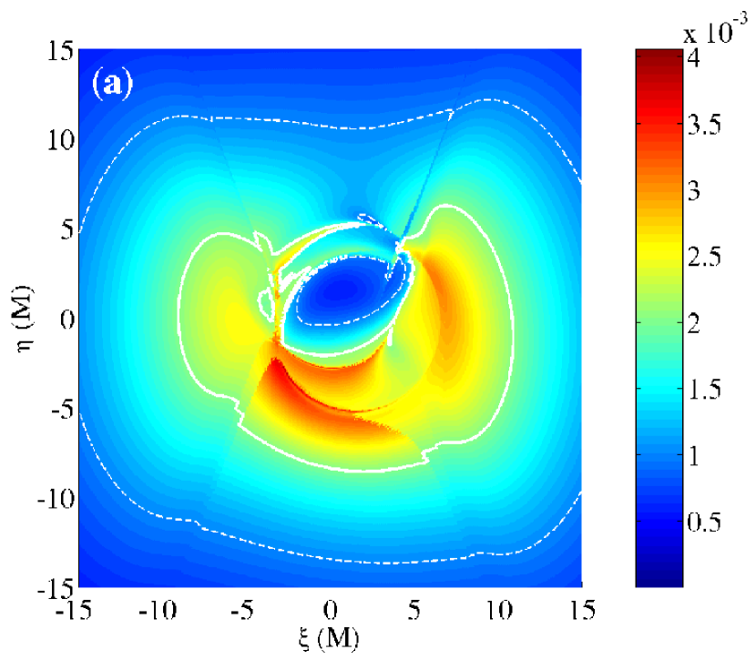
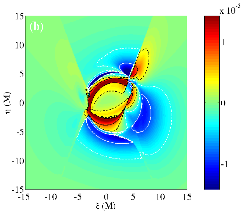
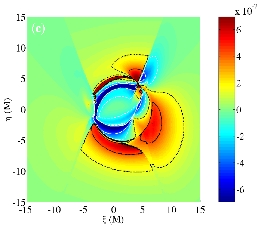
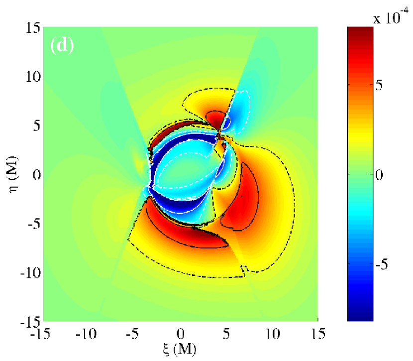
Figure 2: Stokes $I$, $Q$, $U$, and $V$ per unit $M^{2}$ are shown in panels (a), (b), (c), and (d), respectively, for the unpolarised emission mechanism described in section 4.5 and the disk model described in section 5.1 and appendix A orbiting a maximally rotating black hole from a vantage point $45^{\circ}$ above the equatorial plane at the frequency $\omega_{\infty}=3\omega_{P,{\rm max}}/4$. The contour levels are at 0.2 (dashed) and 0.6 (solid) of the maximum values shown on the associated colorbars. The integrated fluxes over the region shown are $I=1.3$, $Q=-9.4\times 10^{-4}$, $U=4.9\times 10^{-5}$, and $V=6.2\times 10^{-2}$. All fluxes are in units of $(M/D)^{-2}\omega_{P\,{\rm max}}^{2}$ as discussed above equation (53).

Figure 2 may be compared with Figure 3 in which Stokes $I$, $Q$, $U$, and $V$ are shown at $\omega_{\infty}=3\omega_{P\,{\rm max}}$ for the same unpolarised emission model. In the latter case the refractive effects are significantly repressed. This demonstrates the particularly limited nature of the frequency regime in which these types effects can be expected to occur. In this case there still does exist a net circular polarisation, now with integrated values $I=1.0$, $Q=-4.8\times 10^{-6}$, $U=2.4\times 10^{-7}$, and $V=1.2\times 10^{-3}$.

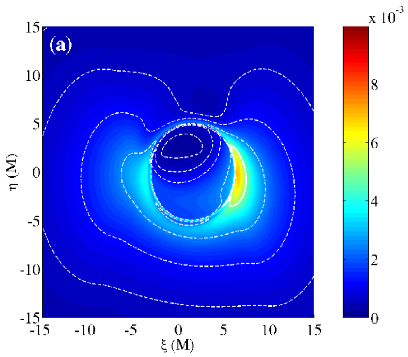
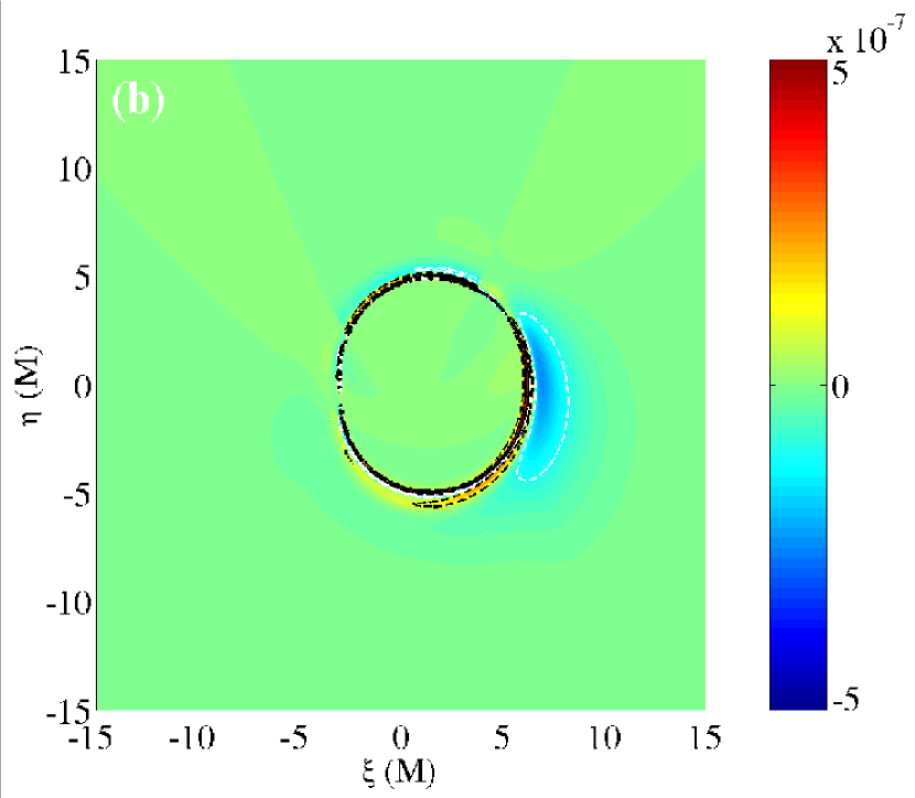
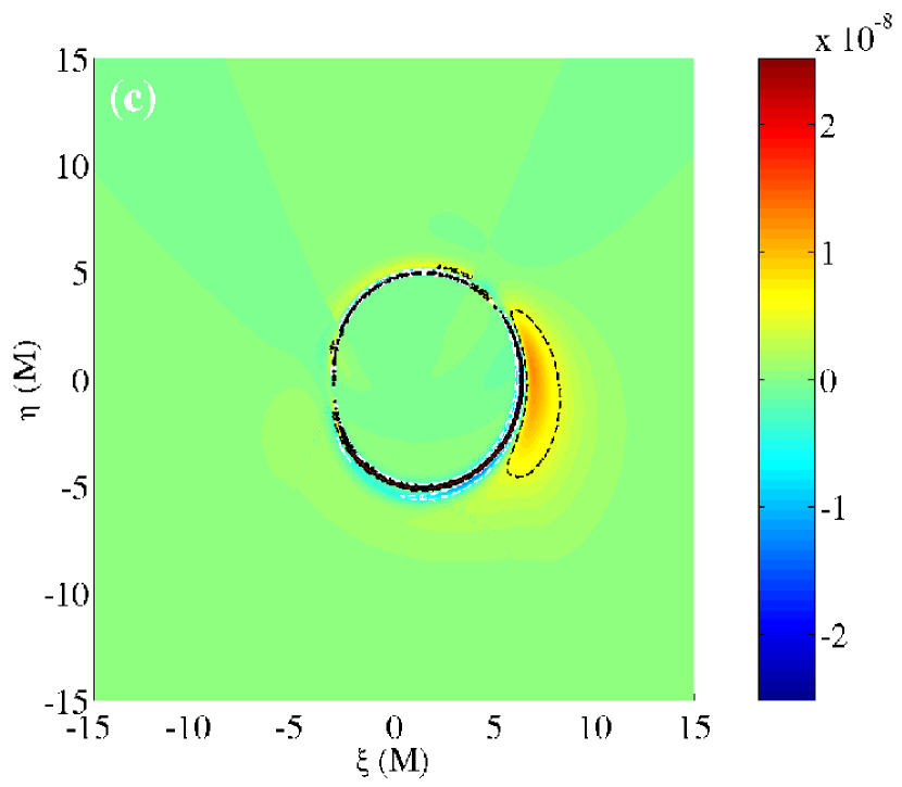
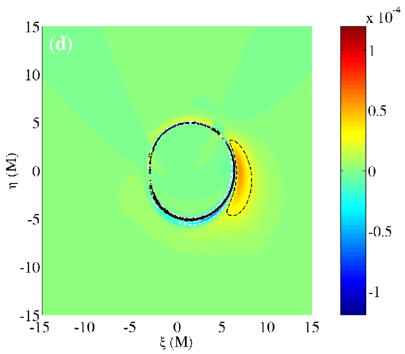
Figure 3: Same as Figure 2 except with $\omega_{\infty}=3\omega_{P\,{\rm max}}$. The integrated fluxes over the region shown are $I=1.0$, $Q=-4.8\times 10^{-6}$, $U=2.4\times 10^{-7}$, and $V=1.2\times 10^{-3}$. All fluxes are in units of $(M/D)^{-2}\omega_{P\,{\rm max}}^{2}$ as discussed above equation (53).

5.3.2 Polarised Emission

In general, synchrotron emission will be polarised. As a result it is necessary to produce polarisation maps using the emission model described in sections 4.3 and 4.4. In this case a net polarisation will exist even in the absence of any refraction. In order to compare the amount of polarisation generated by refractive effects to that created intrinsically, Figure 4 shows Stokes $I$, $Q$, $U$, and $V$ calculated using the polarised emission model and ignoring refraction (i.e. setting the rays to be null geodesics) for $\omega_{\infty}=3\omega_{P,{\rm max}}/4$. Strictly speaking, this is a substantial over estimate of the polarisation. This is because, in the absence of refraction, in principle it is necessary to include Faraday rotation and conversion in the transfer effects considered. As a result of the high plasma density and magnetic field strengths, the Faraday rotation and conversion depths for this system should be tremendous for non-refractive rays, effectively depolarising any emission.

In comparison to Figures 2 and 3, the general morphology of the polarisation maps are substantially different. In addition, the amount of linear polarisation is significantly larger, having an integrated value of over 60% compared to less than 0.1% in Figure 2 and less than $10^{-3}$% in Figure 3. This calculation can be compared to that done by Bromley et al., 2001. In both it was assumed that the rays were null geodesics. In both Faraday rotation/conversion were neglected (in Bromley et al., 2001 because for their disk model it was assumed to be negligible.) However, in Bromley et al., 2001 it was also assumed that the radiative transfer could always be done in the adiabatic regime. As a result, the net polarisation was determined entirely by the emission mechanism. However, as discussed in section 3.1 this is only possible in the strongly coupled regime. In this case, the dichroic terms in equation (42) provide the source of circular polarisation, even in the absence of a circularly polarised emission, resulting from the different absorption properties of the two polarisation eigenmodes. This is what leads to the presence of circular polarisation in Figure 4 but not in Bromley et al., 2001. In this case, the integrated values of the Stokes parameters are $I=1.1$, $Q=6.0\times 10^{-1}$, $U=-4.9\times 10^{-3}$, and $V=6.9\times 10^{-2}$. The vertical feature directly above the black hole in panels (b) and (c) are associated with the rapid decrease in the magnetic field strength in the evacuted funnel above and below the black hole and are due to the geometric transfer effect discussed in section 3.3.

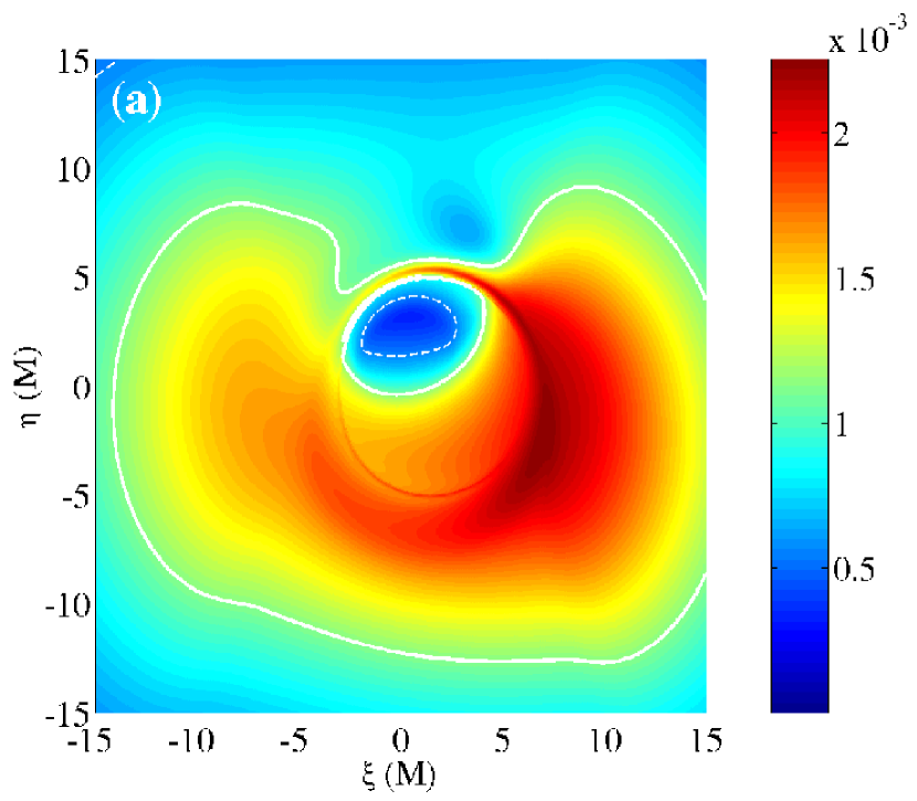
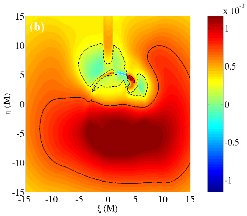
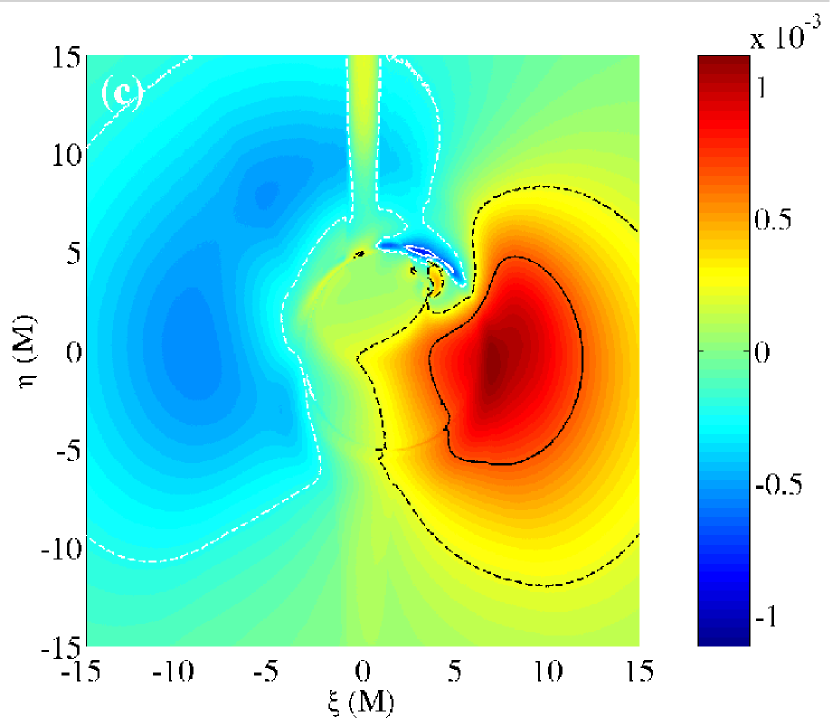
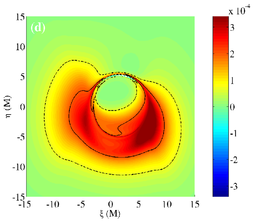
Figure 4: Same as Figure 2 except using the polarised emission mechanism (described in sections 4.3 and 4.4) and ignoring refractive plasma effects. The integrated fluxes over the region shown are $I=1.1$, $Q=6.0\times 10^{-1}$, $U=-4.9\times 10^{-3}$, and $V=6.9\times 10^{-2}$. All fluxes are in units of $(M/D)^{-2}\omega_{P\,{\rm max}}^{2}$ as discussed above equation (53).

Finally, in Figure 5, both refractive effects and the polarised emission mechanism are included (again at $\omega_{\infty}=3\omega_{P,{\rm max}}/4$). Many of the qualitative features of Figure 2 still persist. The integrated values of the Stokes parameters are $I=1.3$, $Q=-2.2\times 10^{-3}$, $U=1.2\times 10^{-4}$, and $V=1.4\times 10^{-1}$. While the intrinsic polarisation in the emission does make a quantitative difference, it is clear that in this case the generic polarimetric properties are dominated by the refractive properties. This is most clearly demonstrated by noting the strong supression of linear polarisation. In Figure 5 the linear polarisation fraction is less than 0.2% as compared with nearly 60% in Figure 4.

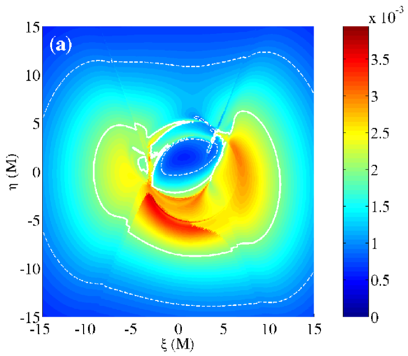
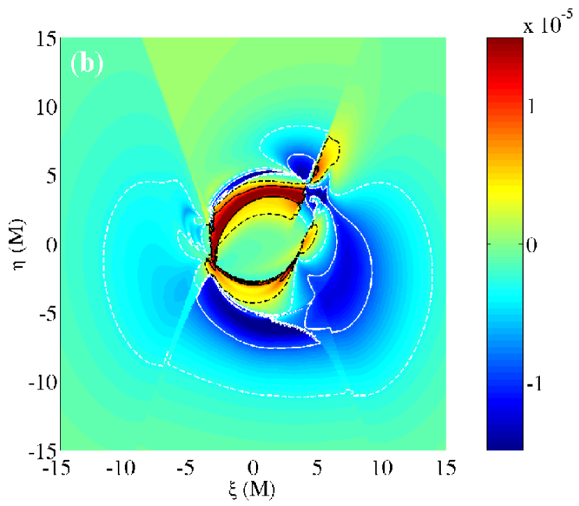
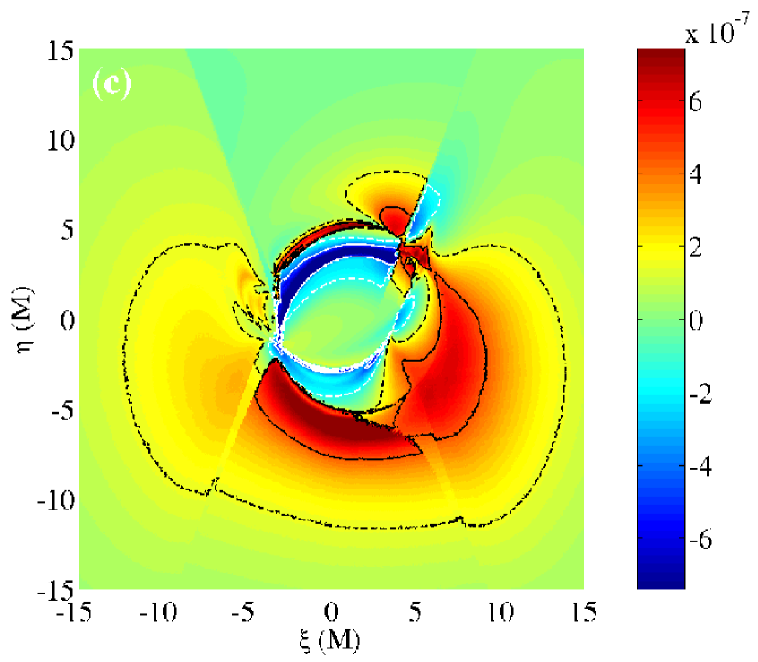
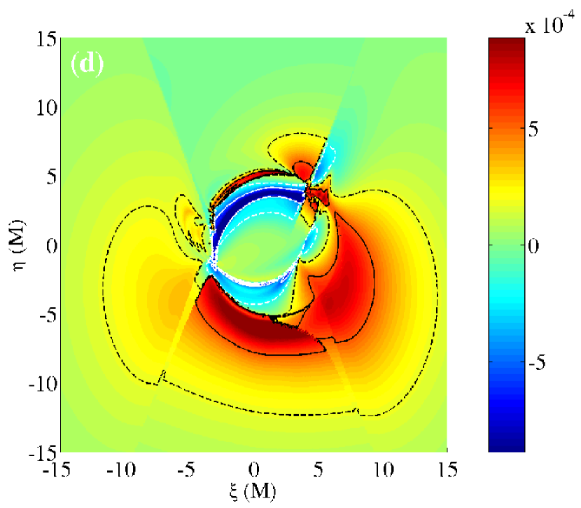
Figure 5: Same as Figure 4 except including refractive plasma effects. The integrated fluxes over the region shown are $I=1.3$, $Q=-2.2\times 10^{-3}$, $U=1.2\times 10^{-4}$, and $V=1.4\times 10^{-1}$. All fluxes are in units of $(M/D)^{-2}\omega_{P\,{\rm max}}^{2}$ as discussed above equation (53).

5.4 Integrated Polarisations

Figure 6 shows the Stokes parameters as a function of frequency for when only polarised emission is considered, only refractive plasma effects are considered, and when both are considered. There are two notable effects due to refraction: (i) the significant suppression of the linear polarisation, and (ii) the large amplification of circular polarisation. The linear polarisation is decreased by at least two orders of magnitude, and in particular, at least two orders of magnitude less than the final circular polarisation. On the other hand, the circular polarisation is more than doubled at its peak, and increases by many orders of magnitude at higher frequencies. Nonetheless, by $\omega_{\infty}=10\omega_{P\,{\rm max}}$, both polarisations are less than one tenth of their maxima. As a result, it is clear that this mechanism is restricted to approximately one decade in frequency, centred about $\omega_{P\,{\rm max}}$.

Figure 6: The log of the integrated intensity, total linear polarisation, and circular polarisation are shown as a function of the observation frequency at infinity for when only polarised emission is considered (open triangles), only refractive plasma effects are considered (open squares), and when both are considered (filled circles). As in Figures 1-5, the disk model described in section 5.1 and appendix A orbiting a maximally rotating black hole is viewed from a vantage point $45^{\circ}$ above the equatorial plane. All fluxes are in units of $(M/D)^{-2}\omega_{P\,{\rm max}}^{2}$ as discussed above equation (53).

Figure 7 shows the circular polarisation fraction as a function of frequency for the same set of cases that were depicted in the previous figure. As can be seen in Figure 6, the circular and linear polarisation spectral index are approximately equal, and both are softer than that of the total intensity. The result is a decreasing circular polarisation fraction with increasing frequency.

Figure 7: Shown is the circular polarisation fraction as a function of the observation frequency at infinity for when only polarised emission is considered (open triangles), only refractive plasma effects are considered (open squares), and when both are considered (filled circles). As in Figures 1-6, the disk model described in section 5.1 and appendix A orbiting a maximally rotating black hole is viewed from a vantage point $45^{\circ}$ above the equatorial plane.

6 Conclusions

We have presented refraction as a mechanism for the generation of polarisation when $\omega_{\infty}\sim\omega_{P},\,\omega_{B}$. That this will typically result in mostly circular polarisation is a result of the fact that the polarisation eigenmodes are significantly elliptical only when the wave-vector and the magnetic field are within $\omega_{B}/\omega$ of perpendicular, which is usually a small number near the surface where the polarisation freezes out. In addition to producing circular polarisation, this mechanism also significantly suppresses linear polarisation. Because it does require significant refraction to take place, it is necessarily limited to approximately a decade in frequency, making it simple to identify.

As shown in section 5.4, the resulting circular polarisation will be softer than the intensity. However, because of optical depth effects, as the observation frequency increases the polarimetric properties of such a system will be dominated be increasingly smaller areas. As a result, the fractional variability in such a system would be expected to increase with frequency. Furthermore, even though the emission may arise from a large region, the polarimetric properties will continue to be determined by this compact area, making it possible to have variability on time scales short in comparison to those associated with the emission region. In addition, variability in the circular polarisation would be expected to be correlated with variability in the integrated intensity at frequencies where the emission is dominated by contributions from close to the horizon (e.g. X-rays).

Possible applications to known astrophysical sources include the Galactic Centre (at submm wavelengths) and extinct high mass X-ray binaries (in the infrared). These will be disscussed in further detail in an upcoming paper.

Appendix A A Thick Disk Model

In general, the innermost portions of the accretion flow will take the form of a thick disk. The equation for hydrostatic equilibrium in the limit that $\Omega\gg v_{r}$ is given by

$$\frac{\partial_{\mu}P}{\rho+\frac{\Gamma}{\Gamma-1}P}=-\partial_{\mu}\ln E+\frac{\Omega\partial_{\mu}L}{1-\Omega L}\,,$$ (55)

where here $\Gamma$ is the adiabatic index, $E=-\overline{u}_{t}$, $\Omega=\overline{u}^{\phi}/\overline{u}^{t}$, and $L=-\overline{u}_{\phi}/\overline{u}_{t}$ (Blandford & Begelman, 2003). Note that, given the metric, any two of the quantities $E$, $\Omega$, or $L$, may be derived from the third. Explicitly, $\Omega$ and $L$ are related by

$$\Omega=\frac{g^{\phi\phi}L+g^{t\phi}}{g^{tt}+g^{t\phi}L}\,,$$ (56)

and the condition that $\overline{u}^{\mu}\overline{u}_{\mu}=\overline{u}^{t}\overline{u}_{t}+\overline{u}^{\phi}\overline{u}_{\phi}=-1$ gives $E$ in terms of $\Omega$ and $L$ to be

$$E=\left[-\left(g^{tt}+g^{t\phi}L\right)\left(1-\Omega L\right)\right]^{-1/2}\,.$$ (57)

In principle this should be combined with a torque balance equation which explicitly includes the mechanism for angular momentum transport through the disk. However, given a relationship between any two of the quantities $E$, $\Omega$, and $L$ specifies this automatically. Thus the problem can be significantly simplified if such a relationship can be obtained, presumably from the current MHD disk simulations.

A.1 Barotropic Disks

For a barotropic disk the left side of equation (55) can be explicitly integrated to define a function $H$:

$$H=\int\frac{dP}{\rho(P)+\frac{\Gamma}{\Gamma-1}P}\,,$$ (58)

which may be explicitly integrated for gases with constant $\Gamma$ to yield

$$H=\ln\left(1+\frac{\Gamma}{\Gamma-1}\frac{P}{\rho}\right)\,.$$ (59)

Therefore, reorganising equation (55) gives

$$\partial_{\mu}\left(H-\ln E\right)=-\frac{\Omega\partial_{\mu}L}{1-\Omega L}\,,$$ (60)

which in turn implies that $\Omega$ is a function of $L$ alone. Specifying this function allows the definition of another function $\Xi$:

$$\Xi=\int\frac{\Omega(L)dL}{1-\Omega(L)L}\,.$$ (61)

Using their definitions, it is possible to solve $\Omega=\Omega(L)$ for $L(x^{\mu})$ and hence $\Xi(x^{\mu})$. Then $H$ and $\Xi$ are related by,

$$H=H_{0}+\ln E-\Xi\,,$$ (62)

which then may be inverted to yield $\rho(H_{0}-\ln E+\Xi)$. Inverting $H$ for $\rho$ then yields $\rho(x^{\mu})$. The quantity $H_{0}$ sets the density scale and may itself be set by choosing $\rho$ at some point:

$$H_{0}=H(\rho_{0})-(\ln E-\Xi)(x_{0}^{\mu})\,.$$ (63)

A.1.1 Keplerian Disk

As a simple, but artificial, example of the procedure, a Keplerian disk is briefly considered in the limit of weak gravitating Schwarzschild black hole (i.e. $r\gg M$). Note that this cannot be done in flat space because in equation (55) the gravitational terms are present in the curvature only. For a Keplerian flow, $\Omega=\sqrt{M/(r\sin\theta)^{3}}\simeq M^{2}L^{-3}$. In that case using the definition of $\Xi$ gives

$$\Xi =M^{2}\int\frac{dL}{L^{3}-M^{2}L}$$

$$=\int\frac{d\ell}{\ell^{3}-\ell}=\ln\sqrt{1-\ell^{-2}}\,,$$ (64)

where $\ell=L/M$. However, $\ln E$ is given by

$$\ln E=-\ln\sqrt{-g^{tt}(1-\Omega L)}=\ln\sqrt{1-\frac{2M}{r}}-\ln\sqrt{1-\ell^{-2}}\,,$$ (65)

and hence,

$$H =H_{0}-\ln E+\Xi$$

$$=H_{0}-\ln\sqrt{1-\frac{2M}{r}}+\ln\left(1-\ell^{-2}\right)$$

$$\simeq H_{0}+\frac{M}{r}-\frac{M}{r\sin\theta}\,,$$ (66)

where $\ell=\sqrt{r\sin\theta/M}$ and the weakly gravitating condition were used. As expected, along the equatorial plane $H$, and therefore $\rho$, is constant. For points outside of the equatorial plane pressure gradients are required to maintain hydrostatic balance.

A.1.2 Pressure Supported Disk

Accretion disks will in general have radial as well as vertical pressure gradients. Inward pressure gradients can support a stable disk inbetween the innermost stable orbit and the photon orbits, thus decreasing the radius of the inner edge of the disk. Around a Schwarzschild black hole this can bring the inner edge of the disk down to $3M$. In a maximally rotating Kerr spacetime this can allow the disk to extend down nearly to the horizon.

Far from the hole, accreting matter will create outward pressure gradients. An angular momentum profile appropriate for a Kerr hole which goes from being super to sub-Keplerian is

$$L(r_{\rm eq}) =\left\{\begin{array}[]{l}\left.\left(\sqrt{g^{t\phi~{}2}_{~{}~{},r}-g^{tt}_{~{}~{},r}g^{\phi\phi}_{~{}~{},r}}-g^{t\phi}_{~{}~{},r}\right)g^{\phi\phi~{}-1}_{~{}~{},r}\right|_{r=r_{\rm eq}}\\ \quad\quad\quad\quad{\rm if~{}}r_{\rm eq}<r_{\rm inner}\\ \\ c_{1}M^{3/2}r_{\rm eq}^{-1}+c_{2}M^{1/2}+l_{0}\sqrt{Mr_{\rm eq}}\\ \quad\quad\quad\quad{\rm otherwise}\end{array}\right.$$ (72)

$$\Omega(r_{\rm eq}) =\left.\frac{g^{\phi\phi}L+g^{t\phi}}{g^{tt}+g^{t\phi}L}\right|_{r=r_{\rm eq}}\,,$$ (73)

where both $L$ and $\Omega$ are parametrised in terms of the equatorial radius, $r_{\rm eq}$. The condition that $L$ reduces to the angular momentum profile of a Keplerian disk for radii less than the inner radius ensures that no pathological disk structures are created within the photon orbit. The constants $c_{1}$ and $c_{2}$ are defined by the requirement that at the inner edge of the disk, $r_{\rm inner}$, and at the density maximum, $r_{\rm max}$, the angular momentum must equal that of the Keplerian disk. In contrast, $l_{0}$ is chosen to fix the large $r$ behaviour of the disk. The values chosen here were $r_{\rm inner}=1.3M$, $r_{\rm max}=2M$, and $l_{0}=0.1$. The value of $H_{0}$ was set so that $H(r_{\rm eq}=100M)=0$, thus making the disk extend to $r_{\rm eq}=100M$.

In addition to defining $\Omega$ and $L$ it is necessary to define $P(\rho)$. Because the gas in this portion of the accretion flow is expected to be unable to efficiently cool, $\Gamma=5/3$ was chosen. The proportionality constant in the polytropic equation of state, $\kappa$, is set by enforcing the ideal gas law for a given temperature ($T_{0}$) at a given density ($\rho_{0}$). Thus,

$$P(\rho)=\rho_{0}\frac{kT_{0}}{m_{p}}\left(\frac{\rho}{\rho_{0}}\right)^{5/3}\,.$$ (74)

Note that $\rho_{0}$ and $T_{0}$ provide a density and temperature scale. A disk solution obtained for a given $\rho_{0}$ and $T_{0}$ may be used to generate a disk solution for a different set of scales simply by multiplying the density everywhere by the appropriate constant factor.

Figure 8: Shown are the contours of the density and azimuthal velocity as measured by the zero angular momentum observer, and the magnetic field lines. Starting at the density maximum ($r_{\rm eq}=2M$ and $z=0$), the density is contoured at levels $10^{-0.5}$ to $10^{-4.5}$ times the maximum density in multiples of $10^{-1}$. From left to right, the velocity is contoured at levels $2^{-0.5}c$ to $2^{-5}c$ in multiples of $2^{-0.5}$. In order to provide a distinction between the velocity contours and the magnetic field lines, the velocity contours are terminated at the disks surface.

A.2 Non-Sheared Magnetic Field Geometries

The disk model discussed thus far is purely hydrodynamic. Typically, magnetic fields will also be present. In general, it is necessary to perform a full MHD calculation in order to self-consistently determine both the plasma and magnetic field structure. However,an approximate steady state magnetic field can be constructed by requiring that the field lines are not sheared.

To investigate the shearing between two nearby, space-like separated points in the plasma, $x_{1}^{\mu}$ and $x_{2}^{\mu}$, consider the invariant interval between them:

$$\Delta s^{2}=\Delta x^{\mu}\Delta x_{\mu}\quad{\rm where}\quad\Delta x^{\mu}=x_{2}^{\mu}-x_{1}^{\mu}\,.$$ (75)

The condition that this doesn’t change in the LFCR frame is equivalent to

$$\frac{d\Delta s^{2}}{ds}=0\,.$$ (76)

Expanding in terms of the definition of $\Delta s$ gives,

$$\frac{d}{ds}g_{\mu\nu}\Delta x^{\mu}\Delta x^{\nu}=g_{\mu\nu,\sigma}\frac{dx^{\sigma}}{ds}\Delta x^{\mu}\Delta x^{\nu}\\ +2g_{\mu\nu}\Delta x^{\mu}\frac{d\Delta x^{\nu}}{ds}=0\,.$$ (77)

Note that by definition,

$$\frac{dx^{\mu}}{ds}=\overline{u}^{\mu}\quad{\rm and}\quad\frac{d\Delta x^{\mu}}{ds}=\overline{u}_{2}^{\mu}-\overline{u}_{2}^{\mu}=\overline{u}^{\mu}_{,\sigma}\Delta x^{\sigma}\,.$$ (78)

Hence,

$$\frac{d\Delta s^{2}}{ds} =\left(g_{\mu\nu,\sigma}\overline{u}^{\sigma}+2g_{\mu\sigma}\overline{u}^{\sigma}_{,\nu}\right)\Delta x^{\mu}\Delta x^{\nu}$$

$$=\left(g_{\mu\nu,\sigma}\overline{u}^{\sigma}+2\overline{u}_{\mu,\nu}-2g_{\mu\sigma,\nu}\overline{u}^{\sigma}\right)\Delta x^{\mu}\Delta x^{\nu}$$

$$=2\left(\overline{u}_{\mu,\nu}-\Gamma^{\sigma}_{\mu\nu}\overline{u}_{\sigma}\right)\Delta x^{\mu}\Delta x^{\nu}$$

$$=2\left(\nabla_{\mu}\overline{u}_{\nu}\right)\Delta x^{\mu}\Delta x^{\nu}=0\,.$$ (79)

The final equality is easy to understand from a geometrical viewpoint; for there to be no shearing, there can be no change in the direction of $\Delta x^{\mu}$ of the component of the plasma four-velocity along $\Delta x^{\mu}$.

That a steady state, axially symmetric magnetic field must lie upon the non-shearing surfaces can be seen directly by considering the covariant form of Maxwell’s equations. In particular $\nabla_{\nu}^{*}\!F^{\mu\nu}=0$, where ${}^{*}\!F^{\mu\nu}$ is the dual of the electromagnetic field tensor, which in the absence of an electric field in the frame of the plasma takes the form ${}^{*}\!F^{\mu\nu}={\cal B}^{\mu}\overline{u}^{\nu}-{\cal B}^{\nu}\overline{u}^{\mu}$. Therefore,

$${\cal B}_{\mu}\nabla_{\nu}^{*}\!F^{\mu\nu} ={\cal B}_{\mu}{\cal B}^{\mu}\nabla_{\nu}\overline{u}^{\nu}+{\cal B}_{\mu}\overline{u}^{\nu}\nabla_{\nu}{\cal B}^{\mu}$$

$$\quad-{\cal B}_{\mu}\overline{u}^{\mu}\nabla_{\nu}{\cal B}^{\nu}-{\cal B}_{\mu}{\cal B}^{\nu}\nabla_{\nu}\overline{u}^{\mu}$$

$$=-{\cal B}^{\mu}{\cal B}^{\nu}\nabla_{\nu}\overline{u}_{\mu}=0\,,$$ (80)

where the first three terms vanish due to the symmetries and the requirement that ${\cal B}^{\mu}\overline{u}_{\mu}=0$. This is precisely the non-shearing condition obtained in equation (79).

For plasma flows that are directed along the Killing vectors of the spacetime, $\xi_{i}^{\mu}$, i.e.

$$\overline{u}^{\mu}=u^{t}t^{\mu}+\sum_{i}u^{i}\xi_{i}^{\mu}\,,$$ (81)

where $t^{\mu}$ is the time-like Killing vector, it is possible to simplify the no-shear condition considerably.

$$\Delta x^{\mu}\Delta x_{\nu}\nabla_{\mu}\overline{u}^{\nu}$$

$$\quad=\Delta x^{\mu}\Delta x_{\nu}\left(u^{t}\nabla_{\mu}t^{\nu}+\sum_{i}u^{i}\nabla_{\mu}\xi_{i}^{\nu}\right)$$

$$\quad\quad+\Delta x^{\mu}\Delta x_{\nu}\left(t^{\nu}\partial_{\mu}u^{t}+\sum_{i}\xi_{i}^{\nu}\partial_{\mu}u^{i}\right)$$

$$\quad=\Delta x_{t}\Delta x^{\mu}\partial_{\mu}u^{t}+\sum_{i}\Delta x_{i}\Delta x^{\mu}\partial_{\mu}u^{i}=0\,,$$ (82)

Where terms in the first parentheses vanish due to Killing’s equation. The additional constraint that $\Delta x_{\mu}\overline{u}^{\mu}=0$ gives

$$\Delta x_{t}=-\sum_{i}\Omega_{i}\Delta x_{i}\,,$$ (83)

where $\Omega_{i}\equiv u^{i}/u^{t}$ is a generalisation of the definition of $\Omega$ at the beginning of the section. Inserting this into equation (82) and simplifying yields

$$\sum_{i}\Delta x_{i}\Delta x^{\mu}\partial_{\mu}\Omega_{i}=0\,,$$ (84)

i.e. the no shear hypersurfaces are those upon which all of the $\Omega_{i}$ are constant.

For the plasma flows considered in §A.1 the plasma velocity is in the form of equation (81) where the space-like Killing vector is that associated with the axial symmetry, $\phi^{\mu}$. Thus with $\Omega_{\phi}=\Omega$, the no-shear condition for this class of plasma flows is

$$\Delta x^{\mu}\partial_{\mu}\Omega=0\,.$$ (85)

Note that while we have been considering only axially symmetric plasma flows, this no shear condition is more generally valid, extending to the case where $\Omega$ is a function of $t$ and $\phi$ as well as $r$ and $\theta$. However, in this case it is not the perfect-MHD limit of Maxwell’s equations.

For a cylindrically symmetric disk, the no-shear condition may be used to explicitly construct the non-shearing poloidal magnetic fields by setting

$${\cal B}^{r}={\cal B}\Omega_{,\theta}\quad{\rm and}\quad{\cal B}^{\theta}=-{\cal B}\Omega_{,r}\,.$$ (86)

Once the magnitude of ${\cal B}^{\mu}$ is determined at some point along each non-shearing surfaces (e.g. in the equatorial plane), it may be set everywhere by $\nabla_{\mu}{\cal B}^{\mu}-B^{\mu}\overline{u}^{\nu}\nabla_{\nu}\overline{u}_{\mu}=0$, which comes directly from Maxwell’s equations in covariant form and $B^{\mu}\overline{u}_{\mu}=0$. Inserting the form in equation (86) into the first term gives

$$\nabla_{\mu}{\cal B}^{\mu} =\frac{1}{\sqrt{g}}\partial_{\nu}\sqrt{g}{\cal B}^{\nu}$$

$$=\frac{1}{\sqrt{g}}\left(\partial_{r}\sqrt{g}{\cal B}\Omega_{,\theta}-\partial_{\theta}\sqrt{g}{\cal B}\Omega_{,r}\right)$$

$$=\frac{1}{\sqrt{g}}\left(\Omega_{,\theta}\partial_{r}\sqrt{g}{\cal B}-\Omega_{,r}\partial_{\theta}\sqrt{g}{\cal B}\right)$$

$$={\cal B}^{\nu}\partial_{\nu}\ln\sqrt{g}{\cal B}\,.$$ (87)

The second term can be simplified using equation (81),

$${\cal B}^{\mu}\overline{u}^{\nu}\nabla_{\nu}\overline{u}_{\mu} ={\cal B}^{\mu}\overline{u}^{\nu}\nabla_{\nu}\left(u^{t}t_{\mu}+u^{\phi}\phi_{\mu}\right)$$

$$={\cal B}^{\mu}\overline{u}^{\nu}\left(t_{\mu}\partial_{\nu}u^{t}+\phi_{\mu}\partial_{\nu}u^{\phi}-u^{t}\nabla_{\mu}t_{\nu}-u^{\phi}\nabla_{\mu}\phi_{\nu}\right)$$

$$={\cal B}_{t}\overline{u}^{\nu}\partial_{\nu}u^{t}+{\cal B}_{\phi}\overline{u}^{\nu}\partial_{\nu}u^{\phi}+{\cal B}^{\mu}\overline{u}^{\nu}\left(t_{\nu}\partial_{\mu}u^{t}\phi_{\nu}\partial_{\mu}u^{\phi}\right)$$

$$\quad+{\cal B}^{\mu}\overline{u}^{\nu}\nabla_{\mu}\overline{u}_{\nu}$$

$$={\cal B}^{\mu}\left(\overline{u}_{t}\partial_{\mu}u^{t}+\overline{u}_{\phi}\partial_{\mu}u^{t}\Omega\right)$$

$$={\cal B}^{\mu}\left(\overline{u}_{t}+\Omega\overline{u}_{\phi}\right)\partial_{\mu}u^{t}+\overline{u}_{\phi}u^{t}{\cal B}^{\mu}\partial_{\mu}\Omega$$

$$=-{\cal B}^{\mu}\partial_{\mu}\ln u^{t}\,,$$ (88)

where the stationarity and axially symmetry have been used in the third step and the no-shear condition was used in the final step. Therefore, the magnitude ${\cal B}$ can be determined by

$$\nabla_{\mu}{\cal B}^{\mu}-B^{\mu}\overline{u}^{\nu}\nabla_{\nu}\overline{u}_{\mu} ={\cal B}^{\mu}\partial_{\mu}\ln\sqrt{g}{\cal B}-{\cal B}^{\mu}\partial_{\mu}\ln u^{t}$$

$$={\cal B}^{\mu}\partial_{\mu}\ln\frac{\sqrt{g}{\cal B}}{u^{t}}=0\,,$$ (89)

and hence

$$\frac{\sqrt{g}{\cal B}}{u^{t}}={\rm constant}$$ (90)

along the non-shearing surfaces. If ${\cal B}$ is given along a curve which passes through all of the non-shearing surfaces (e.g. in the equatorial plane), ${\cal B}^{\mu}$ is defined everywhere through equations (86) and (90).

A.2.1 Non-Shearing Magnetic Fields in a Cylindrical Flow

An example application of this formalism is a cylindrical flow in flat space. In this case, $\Omega$ is a function of the cylindrical radius $\varpi\equiv r\sin\theta$. The Keplerian disk is a specific example with $\Omega=\varpi^{-3/2}$. The direction of the magnetic field is determined by,

$$\Omega_{,r}=\frac{d\Omega}{d\varpi}\sin\theta\quad\quad{\rm and}\quad\quad\Omega_{,\theta}=\frac{d\Omega}{d\varpi}r\cos\theta\,.$$ (91)

The magnitude, ${\cal B}$ is given by

$$\frac{r^{2}\sin\theta}{\sqrt{1-r^{2}\sin^{2}\theta\Omega^{2}}}{\cal B}=f(\Omega)\,,$$ (92)

and thus

$${\cal B}=\frac{1}{r}b(\varpi)\,,$$ (93)

where the particular form of $b(\varpi)$ depends upon the particular form of $f(\Omega)$. Therefore,

$${\cal B}^{r}=b(\varpi)\cos\theta\quad\quad{\rm and}\quad\quad{\cal B}^{\theta}=-b(\varpi)\frac{1}{r}\sin\theta\,,$$ (94)

which is precisely the form of a cylindrically symmetric vertical magnetic field.

A.2.2 Stability to the Magneto-Rotational Instability

A sufficiently strong non-shearing magnetic field configuration will remain stable to the magneto-rotational instability (MRI). The criterion for instability to the MRI is

$$\left({\bf k}\cdot{\bf v}_{\rm A}\right)^{2}<-r\frac{d\Omega^{2}}{dr}\,,$$ (95)

where $\bf{k}$ is the wave vector of the unstable mode and $\bf{v}_{\rm A}$ is the Alfvén velocity (Hawley & Balbus, 1995). For a nearly vertical magnetic field geometry, stability will be maintained if modes with wavelength less than twice the disk height ($h$) are not unstable. With

$$v_{\rm A}=\frac{B}{\sqrt{4\pi\rho}}=\frac{\omega_{B}}{\omega_{P}}\sqrt{\frac{m_{e}}{m_{P}}}\,c\,,$$ (96)

a Keplerian disk will be stable if

$$\frac{4\pi}{h}\frac{\omega_{B}}{\omega_{P}}\sqrt{\frac{m_{e}}{m_{P}}}\,c>\sqrt{3}\left(\frac{M}{r}\right)^{3/2}\frac{c}{M}\,.$$ (97)

A conservative criterion may be obtained by approximating $h\simeq h_{0}r$ for some constant of proportionality $h_{0}$, hence

$$\frac{\omega_{B}}{\omega_{P}}\ga 6h_{0}\sqrt{\frac{M}{r}}\simeq 0.3\,,$$ (98)

for $h_{0}\simeq 0.1$ and $r\simeq 7$ which are typical for the disk pictured in Figure 8.

Comparison to equipartion fields can provide some insight into how unrestrictive the stability criterion really is. Given $\beta=P_{\rm gas}/P_{\rm mag}$ and the ideal gas law it is straight forward to show that

$$\frac{\omega_{B}}{\omega_{P}}=\sqrt{\frac{2kT}{\beta m_{e}c^{2}}}\simeq\sqrt{3\beta^{-1}T_{10}}\,,$$ (99)

where $T$ is the ion temperature. Because the ion temperature in a thick disk will typically be on the order of or exceed $10^{12}$ K, the equipartition $\omega_{B}$ ($\beta=1$) will be at least an order of magnitude larger than $\omega_{P}$. As a result the field needed to stabilise the disk against the MRI is an order of magnitude less than equipartition strength, and hence is not physically unreasonable.

A.2.3 Magnetic Field Model

Considering the restriction placed upon the magnetic field strength discussed in the previous sections, ${\cal B}$ was set such that in the equatorial plane

$$\omega_{B}=\omega_{P}+\eta\left(r+10M\right)^{-5/4}\,,$$ (100)

where the second term provides a canonical scaling at large radii. Here $\eta$ was chosen to be $0.01$.

References

- Agol (1997) Agol E., 1997, Ph.D. Thesis, pp 2+
- Arons & Barnard (1986) Arons J., Barnard J. J., 1986, ApJ, 302, 120
- Barnard & Arons (1986) Barnard J. J., Arons J., 1986, ApJ, 302, 138
- Bekefi (1966) Bekefi G., 1966, Radiation Processes in Plasma Physics. New York: Wiley, 1966
- Blandford & Begelman (2003) Blandford R. D., Begelman M. C., 2003, astro-ph/0306184
- Boyd & Sanderson (1969) Boyd T. J. M., Sanderson J. J., 1969, Plasma Dynamics. Thomas Nelson and Sons LTD, London
- Broderick & Blandford (2003) Broderick A., Blandford R., 2003, MNRAS
- Bromley et al. (2001) Bromley B. C., Melia F., Liu S., 2001, ApJL, 555, L83
- Budden (1952) Budden K. G., 1952, Proc. Roy. Soc.
- Budden (1964) Budden K. G., 1964, Lectures on Magnetoionic Theory. Gordon and Breach, New York
- Connors et al. (1980) Connors P. A., Stark R. F., Piran T., 1980, ApJ, 235, 224
- Ginzburg (1970) Ginzburg V. L., 1970, The propagation of electromagnetic waves in plasmas. International Series of Monographs in Electromagnetic Waves, Oxford: Pergamon, 1970, 2nd rev. and enl. ed.
- Hawley & Balbus (1995) Hawley J. F., Balbus S. A., 1995, Publications of the Astronomical Society of Australia, 12, 159
- Heyl et al. (2003) Heyl J. S., Shaviv N. J., Lloyd D., 2003, MNRAS, 342, 134
- Jones & O’Dell (1977a) Jones T. W., O’Dell S. L., 1977a, ApJ, 214, 522
- Jones & O’Dell (1977b) Jones T. W., O’Dell S. L., 1977b, ApJ, 215, 236
- Laor et al. (1990) Laor A., Netzer H., Piran T., 1990, MNRAS, 242, 560
- Melrose & Gedalin (2001) Melrose D. B., Gedalin M., 2001, Phys. Rev. E, 64, 027401
- Petrova (2000) Petrova S. A., 2000, A&A, 360, 592
- Petrova (2002) Petrova S. A., 2002, A&A, 383, 1067
- Ruszkowski & Begelman (2002) Ruszkowski M., Begelman M. C., 2002, ApJ, 573, 485
- Rybicki & Lightman (1979) Rybicki G. B., Lightman A. P., 1979, Radiative processes in astrophysics. New York, Wiley-Interscience, 1979. 393 p.
- Sazonov (1969) Sazonov V. N., 1969, JETP, 56, 1075
- Sazonov & Tsytovich (1968) Sazonov V. N., Tsytovich V. N., 1968, Radiofizika, 11, 1287
- Shaviv et al. (1999) Shaviv N. J., Heyl J. S., Lithwick Y., 1999, MNRAS, 306, 333
- Weltevrede et al. (2003) Weltevrede P., Stappers B. W., Horn L. J. v. d., Edwards R. T., 2003, astro-ph/0309578
- Westfold (1959) Westfold K. C., 1959, ApJ, 130, 241