Probing the magnetic field with molecular ion spectra - II

Abstract

We present further observational evidence in support of our earlier proposal (Houde et al., 2000) for detecting the presence of the magnetic field in molecular clouds by comparing spectra of molecular ions with those of neutral molecules. The ion lines tend to be narrower and do not show the wings due to flows, when the magnetic field is sufficiently strong. We obtained spectra for the optically thin lines of the H¹³CN and H¹³CO⁺ species in a sample of ten molecular clouds and found the results to be in agreement with our previous observations of the main isotopic species, HCN and HCO⁺, made in OMC1, OMC2, OMC3 and DR21OH, thus eliminating the possibility of optical depth effects playing a role in the ion line narrowing. HCS⁺ was also detected in four of these star forming regions. We also discuss previously published results by Benson et al. (1998) of N₂H⁺ detections in a large sample of dark clouds. We show that the similarity in line widths between ion and neutral species in their sample is consistent with the relatively small amount of turbulence and other flows observed in these clouds.

1 Introduction.

In a previous paper (Houde et al., 2000, hereafter Paper I), we argued that the presence of a magnetic field in a weakly ionized plasma can be detected through comparisons between ion and neutral molecular line profiles. It was shown that, for regions inhabited with a sufficiently strong magnetic field, we expect ions to exhibit narrower line profiles and a significant suppression of high velocity wings in cases where there is non-alignment between the mean field and the neutral flow(s). A further condition is that the flow(s) involved (which could also exist in the form of vorticity, i.e. turbulence) must not have a local zero mean velocity. For a Maxwellian gas velocity distribution there will be no effect.

As supporting evidence for our assertions, we presented observations of HCN, HCO⁺ and N₂H⁺ for the OMC1, OMC2, OMC3 and DR21OH molecular clouds obtained at Caltech Submillimeter Observatory (CSO). In each instance, we observed the effect described above. One could, however, argue that if for some reason the lines of the neutral species were to be significantly more opaque than their ionic counterparts, the differences in the line profiles between the neutrals and ions could simply be the result of greater saturation of the neutral lines rather than the presence of the magnetic field. It would then appear necessary to verify the effect on less abundant species which are more likely to exhibit optically thin lines. This paper addresses this question by presenting detections of H¹³CN and H¹³CO⁺ in a group of ten molecular clouds, including the four studied in Paper I. Furthermore, HCS⁺ was also detected in four of them: OMC3, DR21OH, S140 and W3 IRS5. These detections are important in that they provide comparisons of another ion with a suitable neutral species. We also present HCN, HCO⁺ and N₂H⁺ data for L1551 IRS5. This brings to eleven the number of objects studied so far.

As will be shown, the same effects are observed with the less abundant isotopic species (H¹³CN and H¹³CO⁺); the ion species generally exhibiting narrower line profiles and significantly suppressed wings.

Another argument that could be used to counter our assertions is the importance that chemical differentiation can have on the spectral appearance of different molecular species. In fact, dramatic abundance variations between species have been observed in some molecular cores, as in the case of L1498 (Kuiper et al., 1996), and one might worry that species with different spatial distributions would also exhibit different velocity profiles. But as will be shown, the consistent success of our specific physical model in predicting the relative narrowing of the ion lines renders the need for such chemical postulate less immediate. Moreover, a case can be made against chemical differentiation being the dominant factor in explaining the relative line widths. For example, why are the observed ion lines always narrower, not broader often? Why are the ion lines narrower in cases where the spatial distributions are shown to be the same? Certainly many factors must be taken into account in order to explain the differences in the velocity profiles, but our model’s success in answering questions like these forces us to emphasize the fact that the presence of the magnetic field is most important and, therefore, should not be neglected.

In the last section of the paper, we discuss recent N₂H⁺ observations of dense cores in dark clouds (Benson et al., 1998). As these cores exhibit, on average, narrow line profiles ($\Delta v\sim 0.4$ km/s) and are believed to be primarily thermally supported, they provide us with a good opportunity to test the assertion made in Paper I that there should not be any significant differences between the widths of ion and neutral molecular lines in regions of low turbulence and void of flows.

2 Ion velocity behavior.

It was shown in Paper I that it is possible to calculate the components of the effective velocity of an ion subjected to a flow of neutral particles in a region inhabited with a magnetic field. Under the assumptions that the flow is linear, the plasma is weakly ionized and that all collisions between the ion and the neutrals are perfectly elastic, we get for the mean and variance of the ion velocity components:

$$\left\langle\mathbf{v}_{\|}\right\rangle = \left\langle\mathbf{v}_{\|}^{n}\right\rangle$$ (1)

$$\left\langle\mathbf{v}_{\bot}\right\rangle = \frac{\left\langle\mathbf{v}_{\bot}^{n}\right\rangle+\left\langle\omega_{r}\right\rangle^{-1}\left[\left\langle\mathbf{v}_{\bot}^{n}\right\rangle\times\left\langle\overrightarrow{\omega_{g}}\right\rangle\right]}{1+\left(\frac{\left\langle\overrightarrow{\omega_{g}}\right\rangle}{\left\langle\omega_{r}\right\rangle}\right)^{2}}$$ (2)

$$\sigma_{\|}^{2} = \frac{a\left[\left\langle\left|\mathbf{v}_{\bot}^{n}\right|^{2}\right\rangle-\left\langle\mathbf{v}_{\bot}\right\rangle^{2}\right]+b\left[\sigma_{\|}^{n}\right]^{2}}{\left[\frac{m}{\mu}-1\right]}$$ (3)

$$\sigma_{\bot}^{2} = \frac{g\left[\left\langle\left|\mathbf{v}_{\bot}^{n}\right|^{2}\right\rangle-\left\langle\mathbf{v}_{\bot}\right\rangle^{2}\right]+h\left[\sigma_{\|}^{n}\right]^{2}}{\left[\frac{m}{\mu}-1\right]}$$ (4)

$$\sigma_{T}^{2} = \frac{\left[\left\langle\left|\mathbf{v}_{\bot}^{n}\right|^{2}\right\rangle-\left\langle\mathbf{v}_{\bot}\right\rangle^{2}\right]+\left[\sigma_{\|}^{n}\right]^{2}}{\left[\frac{m}{\mu}-1\right]}$$ (5)

with

$$\left\langle\overrightarrow{\omega_{g}}\right\rangle = \frac{e\left\langle\mathbf{B}\right\rangle}{mc}$$ (6)

$$\left\langle\omega_{r}\right\rangle \simeq \frac{\mu}{m}\nu_{c}$$ (7)

$$\left[\sigma^{n}\right]^{2} = \left\langle\left|\mathbf{v}^{n}\right|^{2}\right\rangle-\left\langle\mathbf{v}^{n}\right\rangle^{2}$$ (8)

$m$ and $\mu$ are the ion mass and the reduced mass. The ion and neutral flow velocities ($\mathbf{v}$ and $\mathbf{v}^{n}$) were broken into two components: one parallel to the magnetic field ($\mathbf{v}_{\|}$ and $\mathbf{v}_{\|}^{n}$) and another ($\mathbf{v}_{\bot}$ and $\mathbf{v}_{\bot}^{n}$) perpendicular to it. $\left\langle\omega_{r}\right\rangle$, $\left\langle\overrightarrow{\omega_{g}}\right\rangle$ and $\nu_{c}$ are the relaxation rate, the mean ion gyrofrequency vector and the (mean) collision rate.

Under the assumption that the neutral flow consists mainly of molecular hydrogen and has a mean molecular mass $A_{n}=2.3$, we get $a\simeq 0.16$, $b\simeq 0.67$, $g=1-a$ and $h=1-b$ (these are functions with a weak dependence on the ion and neutral masses, the values given here apply well to the different ion masses encountered in this paper).

In the “strong” magnetic field limit ($\left\langle\omega_{g}\right\rangle\gg\left\langle\omega_{r}\right\rangle$), the previous set of equations is simplified by the fact that the ion gets trapped in the magnetic field, this implies that $\left\langle\mathbf{v}_{\bot}\right\rangle\sim 0$ (by equation (2)). This condition is probably easily met in a typical cloud where the required magnetic field strength, which scales linearly with the density, can be calculated to be $\left\langle B\right\rangle\gtrsim 1\,\mu$G for a density of $\sim 10^{6}$ cm^-3.

Upon studying the implications of equations (1)-(8), we developed three expectations concerning the differences between the line profiles of coexistent ion and neutral species:

• for regions inhabited with a strong enough magnetic field which is, on average, not aligned with the local flows ($\left\langle\mathbf{v}_{\|}^{n}\right\rangle$ is not dominant), we expect ionic lines to exhibit narrower profiles and a suppression of high velocity wings when compared to neutral lines since $\left\langle\mathbf{v}_{\bot}\right\rangle\sim 0$

• there should be no significant differences between the line profiles when the flows and the mean magnetic field are aligned as the ion velocity is completely determined by $\left\langle\mathbf{v}_{\|}\right\rangle$ (or equivalently $\left\langle\mathbf{v}_{\|}^{n}\right\rangle$)

• a thermal (or microturbulent) line profile would not show any manifestation of the presence of the magnetic field since the mean velocity of the neutral flow is zero.

We refer the reader to Paper I for more details.

2.1 line widths and profiles.

Equations (1)-(8) describe the effect the mean magnetic field has on ions. To derive the line profile for ion species, one could, in principle, apply this set of equations to each and every neutral flow present in a region of a given molecular clouds and project the resulting ion velocities along the line of sight. The sum of all these contributions would give us the observed line profile.

Even though we don’t have such a detailed knowledge of the dynamics of molecular clouds, we can still apply this procedure to the study of simple cases. More precisely, we will concentrate on a given position in a cloud where all the neutral flows are such that they have i) azimuthal symmetry about the axis defined by the direction of the mean magnetic field and ii) reflection symmetry across the plane perpendicular to the same axis. For example, a bipolar outflow would fit this geometry. With these restrictions, we get for the observed ion line profiles:

$$\left\langle v_{obs}\right\rangle = 0$$ (9)

$$\sigma_{obs}^{2} = \sum_{k}C^{k}\left[\left\langle\left|\mathbf{v}_{\|}^{k}\right|^{2}\right\rangle\cos^{2}\left(\alpha\right)+\frac{1}{2}\left\langle\left|\mathbf{v}_{\bot}^{k}\right|^{2}\right\rangle\sin^{2}\left(\alpha\right)\right]$$ (10)

where $\alpha$ is the angle between the direction of the mean magnetic field and the line of sight. The summation runs over every flow contained in any given quadrant of any plane which is perpendicular to the plane of reflection symmetry and which also contains the axis of symmetry. $C^{k}$ is the weight associated with the flow $k$, which presumably scales with the ion density (if the line is optically thin). An equivalent set of equations applies equally well to any coexistent neutral species (which we assume to exist in proportions similar to that of the ion), provided we replace $v_{obs}$ by $v_{obs}^{n}$, $\sigma_{obs}$ by $\sigma_{obs}^{n}$ and $\mathbf{v}^{k}$ by $\left[\mathbf{v}^{n}\right]^{k}$. Using (1)-(8), one can easily verify that these two sets of equations (for neutrals and ions) are identical when the mean magnetic field is negligible ($\left\langle\omega_{g}\right\rangle\ll\left\langle\omega_{r}\right\rangle$).

Under the assumptions that there is no intrinsic dispersion in the neutral flows and that the mean magnetic field is strong ($\left\langle\omega_{g}\right\rangle\gg\left\langle\omega_{r}\right\rangle$), we get for the neutral and ion line widths:

$$\left[\sigma_{obs}^{n}\right]^{2} = \sum_{k}C^{k}\left\langle\left[\mathbf{v}^{n}\right]^{k}\right\rangle^{2}\left[\left\langle\cos\left(\theta^{k}\right)\right\rangle^{2}\cos^{2}\left(\alpha\right)+\frac{1}{2}\left\langle\sin\left(\theta^{k}\right)\right\rangle^{2}\sin^{2}\left(\alpha\right)\right]$$ (11)

$$\sigma_{obs}^{2} \simeq \sum_{k}C^{k}\left\langle\left[\mathbf{v}^{n}\right]^{k}\right\rangle^{2}\left[\rule{0.0pt}{21.52771pt}\left\langle\cos\left(\theta^{k}\right)\right\rangle^{2}\cos^{2}\left(\alpha\right)\right.$$ (12)

$$\,\,\,\,\,\,\,\,\,\,\,\,\left.+\frac{\left\langle\sin\left(\theta^{k}\right)\right\rangle^{2}}{\left[\frac{m}{\mu}-1\right]}\left[a\cos^{2}\left(\alpha\right)+\frac{g}{2}\sin^{2}\left(\alpha\right)\right]\right]$$

where $\theta^{k}$ is the angle between flow $k$ and the axis of symmetry. From equations (11)-(12) one can see that if the flows are aligned with the mean magnetic field ($\theta^{k}\simeq 0$), then neutrals and ions will have similar line widths. On the other hand, when the flows are perpendicular to the field ($\theta^{k}\simeq\frac{\pi}{2}$) the ions have a much narrower profile which scales with their molecular mass as $\left[\frac{m}{\mu}-1\right]^{-\frac{1}{2}}$.

We can further consider the average width one would expect for both kinds of molecular species when a sample of objects is considered. This can be achieved by averaging equations (11)-(12) over the angle $\alpha$ (assuming the sources in the sample to be more or less similar). Assuming that there is no privileged direction in space for the mean magnetic field, we get:

$$\left\langle\left[\sigma_{obs}^{n}\right]^{2}\right\rangle = \frac{1}{3}\sum_{k}C^{k}\left\langle\left[\mathbf{v}^{n}\right]^{k}\right\rangle^{2}$$ (13)

$$\left\langle\sigma_{obs}^{2}\right\rangle \simeq \frac{1}{3}\sum_{k}C^{k}\left\langle\left[\mathbf{v}^{n}\right]^{k}\right\rangle^{2}\left[\left\langle\cos\left(\theta^{k}\right)\right\rangle^{2}+\frac{\left\langle\sin\left(\theta^{k}\right)\right\rangle^{2}}{\left[\frac{m}{\mu}-1\right]}\right]\,.$$ (14)

A variation of the angle $\alpha$ between the mean magnetic field and the line of sight can have a significant effect on the width of the observed ion line profile from a given object (see equation (12)). But this is not necessarily true for neutral species, we can see from equation (11) that the line width is a lot less sensitive to variations in $\alpha$ than that of the ion. The same statements are true for the sample of similar sources (of different orientations) considered here. We can therefore expect the mean width of a neutral line to be larger than its variation between sources and make the following approximation:

$$\frac{\left\langle\sigma_{obs}^{2}\right\rangle}{\left\langle\left[\sigma_{obs}^{n}\right]^{2}\right\rangle}\simeq\left\langle\frac{\sigma_{obs}^{2}}{\left[\sigma_{obs}^{n}\right]^{2}}\right\rangle\,.$$

The term on the right hand side represents the average of the square of the ratio of the ion to neutral line widths. By computing this ratio, one can get an idea of the propensity shown by the flows and the mean magnetic field for alignment with each other.

Going back to equations (13)-(14), we once again see that if the flows are parallel to the field ($\theta^{k}\simeq 0$), the mean ratio of ion to neutral line widths is close to unity. When the flows are perpendicular ($\theta^{k}\simeq\frac{\pi}{2}$) to the field, the square of this ratio is proportional to $\left[\frac{m}{\mu}-1\right]^{-1}$. On the other hand, if the flows don’t have any preferred direction and are randomly oriented (with a uniform distribution) we then find:

$$\left\langle\frac{\sigma_{obs}^{2}}{\left[\sigma_{obs}^{n}\right]^{2}}\right\rangle\simeq\frac{1}{3}\left[1+\frac{2}{\frac{m}{\mu}-1}\right]$$ (15)

which equals 0.38 (0.37) for an ion of molecular mass $A_{i}=30$ (45).

3 Observations of H¹³CN, H¹³CO⁺ and HCS⁺.

In this section we complement our previous observations of HCN, HCO⁺ and N₂H⁺ in OMC1, OMC2, OMC3 and DR21OH with observations of H¹³CN, H¹³CO⁺ and HCS⁺ on a sample of ten objects. These observations are important in that they allow us to ensure that the effect reported in Paper I was not caused by excess saturation of the HCN line profiles. H¹³CN, H¹³CO⁺ and HCS⁺ are substantially less abundant than HCN and HCO⁺, so their emission lines are more likely to be optically thin. Another fundamental reason for the importance of these further observations is that the effects of the magnetic field should be felt by all species of ions. It is therefore desirable to test our concept with observations from as many ion species as possible.

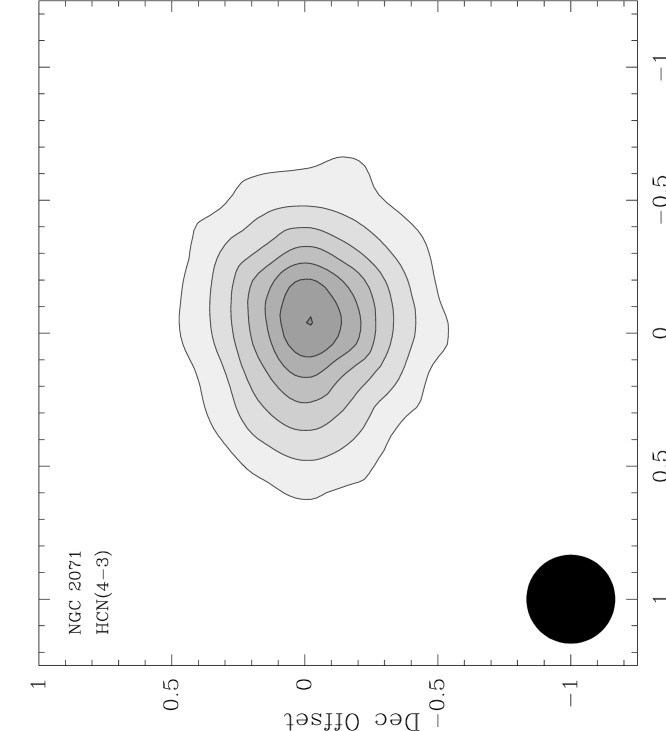
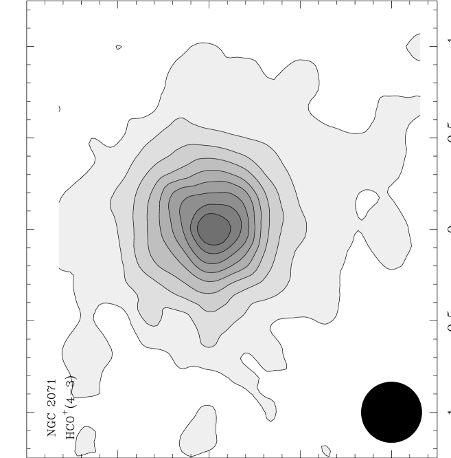
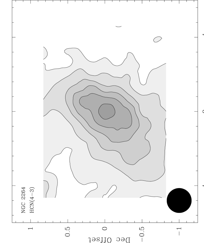
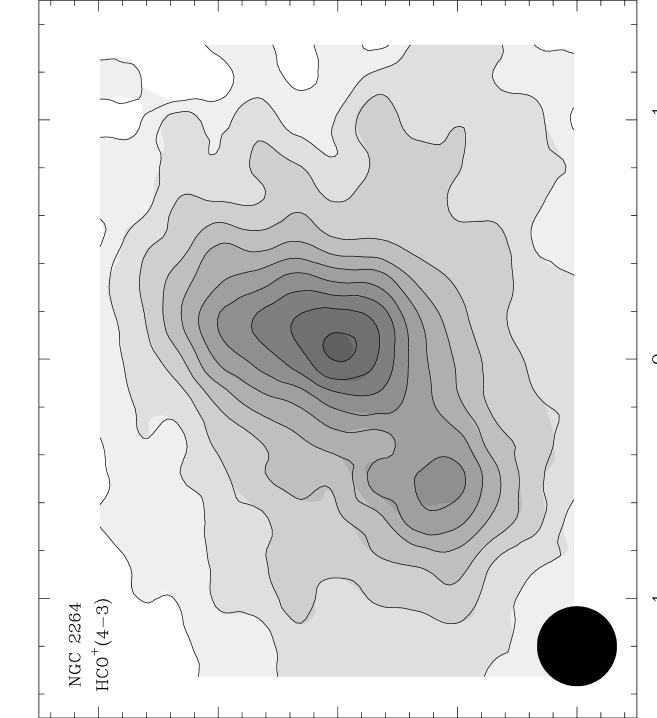
Figure 4: HCN and HCO⁺ ($J\rightarrow 4-3$) maps of NGC 2071 (top) and NGC 2264 (bottom). Although the ion spatial distributions are somewhat more extended, the two peaks are well aligned and the HCN and HCO⁺ systematic velocities agree (from figure 3). The maps for NGC 2071 (NGC 2264) have the same lowest contour level of 5 K$\cdot$km/s (2.5 K$\cdot$km/s) and the following levels increase linearly with an interval of the same amount. The maps’ grid spacing of $10\arcsec$ is half of the beam width (shown in the lower left corners). The pointing accuracy is better than $\sim 5\arcsec$.

We present the spectra in figures 1, 2 and 3. All observations were obtained with the 200-300 GHz and 300-400 GHz receivers at the CSO over a total of fifteen nights during the months of October, November and December 1999. The spectra were calibrated using scans made on planets available during this period (Mars, Jupiter and Saturn). Telescope efficiencies were calculated to be $\sim 70$ % for the 200-300 GHz receiver (beam width of $\sim 32\arcsec$) and $\sim 60$ % for the 300-400 GHz receiver (beam width of $\sim 20\arcsec$). The maps of NGC 2071 and NGC 2264 in HCN and HCO⁺ ($J\rightarrow 4-3$) presented in figure 4 were obtained with the 300-400 GHz receiver in April 1999.

As can be seen, all objects show the line profiles of the ion species as being narrower than those of the neutral species. This is most evident in OMC1, OMC2-FIR4 and W3 IRS5. A suppression of the high velocity wings is the most obvious feature in the case of DR21OH.

Upon closer inspection of the spectra obtained for OMC2-FIR4, we note that the neutral species exhibit profiles that can easily be separated into two components: one narrow line with a FWHM $\sim 1$ km/s that we can associate with the quiescent part of the cloud and a broad feature with a FWHM $\sim 8$ km/s which we assume to be related to (out)flows. On the other hand, the flow component is virtually non-existent in the ion spectra. From this, we can conclude that there is probably a significant misalignment between the direction of the flows and that of the mean magnetic field for this object.

In the case of DR21OH, it is worth noting the striking difference between this set of spectra and the one obtained for the main isotopes (see figure 2 of Paper I). Indeed, a double peaked profile was the most obvious feature in the HCN and HCO⁺ spectra. This was also observed in CN observations by Crutcher et al. (1999) which lead them to identify the peaks as representing two different velocity components and assign two different magnetic field values as measured with the Zeeman effect. But as pointed out before, these molecular species are certainly abundant enough that we should not be surprised if they exhibited strongly self-absorbed line profiles. This effect is well known and can lead to an underestimation of the kinetic temperature of molecular clouds as described, for instance, by Phillips et al. (1981). The fact that the less abundant isotopes do not exhibit the same double peaked profile suggests that this is what is at play in the case of DR21OH and that we are really dealing with a single velocity component.

We present in table 1 a comparison of the line widths (more precisely their standard deviations $\sigma_{v}$) for the different species discussed in this paper, as well as for those studied in Paper I, for our sample of molecular clouds. The widths were measured after the lines were modeled with a multi-Gaussian profile. We have separated the data into four different groups within which the comparison between ion and neutral species should be made. The separations occur naturally and are based on two criteria: i) the perceived optical depth of the lines and ii) the telescope beam applicable to different sets of observations (for example, for H¹³CN (and H¹³CO⁺) in the $J\rightarrow 4-3$ transition, the beam size is $\sim 20\arcsec$ whereas it is $\sim 32\arcsec$ for the lower $J\rightarrow 3-2$ transition). We have also included two detections of H₃O⁺ made on W3 IRS5 by Phillips et al. (1992), these are important since they allow us to test our theory on a different ion species which has a significantly lower molecular mass ($A_{i}=19$).

We have, whenever possible, verified that the opacity of the lines of the H¹³CN, H¹³CO⁺, HCS⁺ and H₃O⁺ species are indeed thin. This was accomplished using the ratio of the line temperature between two different transitions of a given species (assuming LTE and unity beam filling factors (Emerson, 1996)). For example, in the case of the H¹³CO⁺ spectra for OMC2-FIR4 we have line temperatures of 1.9 K and and 1.3 K for the $J\rightarrow 3-2$ and $J\rightarrow 4-3$ transitions respectively. From their ratio and the assumptions made above, we calculated an excitation temperature of $\sim 11$ K (assumed to be the same for both transitions) which then in turn allows us to obtain opacities of $\sim 0.17$ and $\sim 0.12$ for the $J\rightarrow 3-2$ and $J\rightarrow 4-3$ transitions respectively. It should be kept in mind that LTE may not be appropriate for these transitions/sources. Furthermore, the values thus obtained are quite sensitive to the beam filling factors which are probably different for lines observed with different beam sizes. However, we are not seeking a precise value for the opacities, but merely a reassurance that these lines are thin, which this technique provides.

In all cases, the lines were found to be optically thin with the ions generally more opaque than the neutrals, the highest opacity calculated was $\sim 0.3$. One possible exception is the H¹³CN $J\rightarrow 3-2$ line for OMC1, where a comparison with the same transition of the main isotope gives an opacity of $\sim 0.6$. At any rate, it appears that we can safely assume that differences in opacity between ion and neutral lines won’t bring any ambiguity in studying the effects of the magnetic field (see section 1). We can therefore be confident that our widths comparisons are justified.

Upon examination of table 1, we note that in all cases the ion lines exhibit smaller widths ($\sigma_{v}$) than the comparable neutral lines. As was stated in Paper I, this difference in line width could also be partly due to other factors (sampling effect, chemical differentiation, …). But to bring support to the hypothesis that HCN and HCO⁺ are suitable candidate for our study, we discussed observational evidence from the extensive work of Ungerechts et al. (1997), more precisely the fact that their maps of the region surrounding OMC1 for these two molecular species show similar spatial distributions. We, in turn, provided our own maps of OMC2-FIR4 for the same species which also show resemblance in the distributions as well as a good alignment of their respective peaks. We add to the evidence with figure 4 where we again present HCN and HCO⁺ maps in the $J\rightarrow 4-3$ transitions, but this time for NGC 2071 and NGC 2264. The same comments apply for those maps: although the ion spatial distributions are somewhat more extended, the two peaks are well aligned. And from figure 3, we can also attest on the agreement of the systematic velocities for the two species.

If all is well with HCN and HCO⁺, it appears reasonable to assume that the same is true for their less abundant isotopic counterparts H¹³CN and H¹³CO⁺. But we should point out that such comments are probably not true for N₂H⁺ when compared to HCN. It is well known (Bachiller, 1996, 1997) that N₂H⁺ is only observed in the colder condensations of the gas whereas HCN often takes part in outflows, this would automatically result in the former exhibiting narrower line profiles. Our conclusions will, therefore, not be based on comparisons from the data obtained for these two species.

This being said, we interpret the fact that we consistently detect narrower ion line profiles over a sizable sample of molecular clouds for many different ion species as strong evidence in favor of our theory. The ratio of ion to neutral line widths range anywhere from $\sim 0.2$ to $\sim 0.9$ (see table 2), which is not unexpected considering the analysis made in section 2.1. We then showed that ion line widths are strongly dependent on the alignment of the neutral flows with the mean magnetic field (see equation (12)) and are therefore liable to vary from one object to the next. The largest value for this ratio is $\simeq 0.93$ in the case of NGC 2071, implying a good alignment between the field and the flows. Interestingly, this object is known to exhibit strongly collimated jets (Girart et al., 1999, and references therein), this suggests the possibility that these are closely linked to the direction of the mean magnetic field. This aspect will be studied in detail in a subsequent paper.

As a final comment in this section, we point out that the effect of the magnetic field on ion line profiles appears to be roughly similar in importance whether the lines observed are optically thick or thin. This can seen from table 2 where we show the ion to neutral line width ratios for our sample of objects.

3.1 Statistics of the ratios of line widths.

Following our discussion at the end of section 2.1, it is interesting to average the square of the ratio of the ion to neutral line widths over our sample and compare the results with equation (15). We find:

$$\left\langle\frac{\sigma_{\mbox{\scriptsize H}^{13}\mbox{\scriptsize CO}^{+}}^{2}}{\sigma_{\mbox{\scriptsize H}^{13}\mbox{\scriptsize CN}}^{2}}\right\rangle = 0.42$$ (16)

$$\left\langle\frac{\sigma_{\mbox{\scriptsize HCS}^{+}}^{2}}{\sigma_{\mbox{\scriptsize H}^{13}\mbox{\scriptsize CN}}^{2}}\right\rangle = 0.32$$ (17)

which we interpret as meaning that, although this ratio can vary significantly from one object to the next, there is, on average, no obvious propensity for the alignment between the flows and the mean magnetic field in high density molecular clouds such as those studied here. For we know, from the aforementioned discussion, that if the neutral flows don’t have any preferred orientation in relation to the magnetic field, these ratios would be 0.38 for H¹³CO⁺ and 0.37 for HCS⁺. It should, however, be kept in mind that our sample of objects is not entirely composed of (more or less) similar objects, as was assumed when we derived equation (15).

4 Regions of low turbulence.

All the objects discussed so far present a fair amount of turbulence as can be attested by a comparison of the widths of the observed line profiles with their expected thermal width. The former being many times broader than the latter. In fact, as was mentioned earlier we would only expect to observe narrower ion lines in situations where this is the case. According to equations (1)-(8) and (12), we can identify three scenarios for which one should not expect any significant difference between the line widths of ion and neutral species:

• the value of the mean magnetic field is such that $\left\langle\omega_{g}\right\rangle\ll\left\langle\omega_{r}\right\rangle$

• the mean magnetic field is aligned with the flow(s)

• the region under study has little or no (macro)turbulence.

In what follows, we will investigate some observational evidence that, we will argue, show cases where the last scenario is at work.

4.1 Dark clouds with dense cores.

Recently, Benson et al. (1998) studied, among other things, the correlation of the velocity and line widths between the spectra of N₂H⁺ and other neutral species (C₃H₂, CCS and NH₃) on large samples of dark clouds (with dense cores). Their sample contains sources which are very different from those that we have been studying so far in that:

• they have much narrower line profiles, the mean line widths (FWHM) are $0.37$ km/s for N₂H⁺, $0.46$ km/s for C₃H₂, $0.38$ km/s for CCS and $0.36$ km/s for NH₃

• most of the cores are primarily thermally supported, the corresponding thermal width of a neutral molecule of mean mass is $0.45$ km/s at $10$ K

• the densities probed with their observations are roughly two orders of magnitude lower, $n\gtrsim 10^{4}$ cm^-3 in their case compared to $n\gtrsim 10^{6}$ cm^-3 in ours.

As stated before, we expect that regions of low turbulence such as these dark cloud cores would not show significant differences between the width of the line profiles of ion and neutral species. The measured mean line widths reported above seem to indicate that this is the case, only the C₃H₂ species shows a mean line width noticeably different from that of the ion species. However, this situation improves when we limit the comparisons to only those objects which are common to each sample (i.e., the different sets of N₂H⁺, CCS and C₃H₂ observations). This group of objects is listed in table 3 along with the measured line widths. With this restriction, we find that the mean line widths are now 0.36 km/s for N₂H⁺, 0.37 km/s for CCS and 0.41 km/s for C₃H₂. More to the point, if we calculate the root mean square value of the line widths ratios between the different species we get:

$$\sqrt{\left\langle\frac{\Delta v_{\mbox{\scriptsize N}_{2}\mbox{\scriptsize H}^{+}}^{2}}{\Delta v_{\mbox{\scriptsize C}_{3}\mbox{\scriptsize H}_{2}}^{2}}\right\rangle} = 0.90$$

$$\sqrt{\left\langle\frac{\Delta v_{\mbox{\scriptsize N}_{2}\mbox{\scriptsize H}^{+}}^{2}}{\Delta v_{\mbox{\scriptsize CCS}}^{2}}\right\rangle} = 1.05$$

$$\sqrt{\left\langle\frac{\Delta v_{\mbox{\scriptsize CCS}}^{2}}{\Delta v_{\mbox{\scriptsize C}_{3}\mbox{\scriptsize H}_{2}}^{2}}\right\rangle} = 0.97\,.$$

It is therefore evident that the differences in mean line width between ion and neutral species are quite insignificant (compare with equations (16)-(17)). We should point out, however, that we have assumed that all the species are coexistent in the clouds. This is not necessarily true, the authors indeed discuss the lack of correlation between the column densities of N₂H⁺ and those of the neutral species.

It is also worth mentioning that in a recent paper Crutcher (1999) gives upper limits for the component of the magnetic field parallel to the line of sight for a few of the sources studied by Benson et al. (1998). These measurements were obtained using observations of the Zeeman effect in OH emission lines at 1665 and 1667 MHz with a beam size of $18\arcsec$ (Crutcher et al., 1993). The upper limits are all of the order of $\sim 10$ $\mu$G, underlining the relative weakness of the magnetic field.

One might then argue that, according to equations (1)-(8), perhaps the field strength is too low to cause any narrowing in the lines profiles of ions. But since we know that this manifestation should be apparent in the strong magnetic field limit ($\sim 0.01$ $\mu$G at a density of $\sim 10^{4}$ cm^-3, which is well below the typical value measured in the interstellar medium (Heiles, 1987)), it is probably safe to assume that the low level of turbulence and other flows is the cause for the similarity between the ion and neutral spectral widths and not the weakness of the field.

5 Conclusion.

We have presented new observational evidence that helps to verify our assertions that the presence of a sufficiently strong magnetic field in a weakly ionized and turbulent plasma leads to ions exhibiting narrower line profiles and significantly suppressed high velocity wings when compared to neutral lines.

The effect was verified by comparing optically thin transitions of H¹³CN, H¹³CO⁺ and HCS⁺ made on a sample of ten high density molecular clouds. The results are in agreement with our previous observations (Paper I) of probably optically thick lines detected in OMC1, OMC2, OMC3 and DR21OH.

We also discussed the comparison of the line widths of N₂H⁺, CCS, C₃H₂ and NH₃ made on samples of cold and primarily thermally supported clouds previously published by Benson et al. (1998). We show that the lack of a significant difference between the widths of ion to neutral lines is exactly what would be expected for this type of object and therefore confirm a different aspect of our concept presented in Paper I.

Figure 1: H¹³CN , H¹³CO⁺ and HCS⁺ (for DR21OH and OMC3-MMS6) observations at the center position of (clockwise starting from top left): OMC1, OMC2-FIR4, OMC3-MMS6 and DR21OH.

Figure 2: H¹³CN , H¹³CO⁺ and HCS⁺ (for S140 and W3 IRS5) observations at the center position of (clockwise starting from top left): M17SWN, M17SWS, S140 and W3 IRS5.

Figure 3: HCN, HCO⁺, N₂H⁺, H¹³CN and H¹³CO⁺ observations at the center position of NGC 2071 (left) and NGC 2264 (right).

Table 1: line widths in star formation regions.

	$\sigma_{v}$ (km/s)				$\sigma_{v}$ (km/s)				$\sigma_{v}$ (km/s)					$\sigma_{v}$ (km/s)
	HCN	HCO+	N2H+		HCN	HCO+	N2H+		H13CN	H13CO+	H3O+	H3O+		H13CN	H13CO+	HCS+	HCS+
Source	$4-3$	$4-3$	$4-3$		$3-2$	$3-2$	$3-2$		$4-3$	$4-3$	$3^{+}_{0}-2^{-}_{0}$	$3^{+}_{2}-2^{-}_{2}$		$3-2$	$3-2$	$6-5$	$5-4$
W3 IRS5	6.88	2.96	$\cdots$		$\cdots$	$\cdots$	$\cdots$		5.25	1.51	2.38	2.38		4.25	1.99	1.21	1.20
L1551 IRS5	1.03	0.92	0.94		$\cdots$	$\cdots$	$\cdots$		$\cdots$	$\cdots$	$\cdots$	$\cdots$		$\cdots$	$\cdots$	$\cdots$	$\cdots$
OMC3-MMS6	1.40	0.71	0.56		1.25	0.79	$\cdots$		$\cdots$	0.40	$\cdots$	$\cdots$		0.98	0.47	0.51	0.55
OMC1	$\cdots$	$\cdots$	$\cdots$		17.42	3.23	1.87		$\cdots$	$\cdots$	$\cdots$	$\cdots$		8.55	1.85	$\cdots$	$\cdots$
OMC2-FIR4	3.59	2.72	1.34		$\cdots$	$\cdots$	$\cdots$		3.33	1.05	$\cdots$	$\cdots$		3.02	0.65	$\cdots$	$\cdots$
NGC 2071	3.98	3.69	1.18		$\cdots$	$\cdots$	$\cdots$		3.12	2.01	$\cdots$	$\cdots$		$\cdots$	$\cdots$	$\cdots$	$\cdots$
NGC 2264	1.88	1.60	1.38		$\cdots$	$\cdots$	$\cdots$		1.04	0.92	$\cdots$	$\cdots$		$\cdots$	$\cdots$	$\cdots$	$\cdots$
M17SWN	3.29	2.96	1.82		$\cdots$	$\cdots$	$\cdots$		2.82	1.91	$\cdots$	$\cdots$		2.19	2.03	$\cdots$	$\cdots$
M17SWS	2.04	1.84	1.32		$\cdots$	$\cdots$	$\cdots$		0.89	0.69	$\cdots$	$\cdots$		1.51	1.19	$\cdots$	$\cdots$
DR21OH	5.75	4.61	2.08		$\cdots$	$\cdots$	2.41		2.95	1.93	$\cdots$	$\cdots$		2.82	2.04	1.86	1.72
S140	2.69	2.14	1.34		$\cdots$	$\cdots$	$\cdots$		1.50	1.36	$\cdots$	$\cdots$		1.42	1.12	1.09	0.90

Table 2: Ion to neutral width ratios in star formation regions.

	Coordinates (1950)		$v$	$\langle$ratio$\rangle$
Source	RA	DEC	(km/s)	thick	thin
W3 IRS5	$2^{\mathrm{h}}21^{\mathrm{m}}53\fs 3$	$61\arcdeg 52\arcmin 21\farcs 4$	$-38.1$	0.43	0.39
L1551 IRS5	$4^{\mathrm{h}}28^{\mathrm{m}}40\fs 2$	$18\arcdeg 01\arcmin 41\farcs 0$	6.3	0.89	$\cdots$
OMC1	$5^{\mathrm{h}}32^{\mathrm{m}}47\fs 2$	$-05\arcdeg 24\arcmin 25\farcs 3$	9.0	0.19	0.22
OMC3-MMS6	$5^{\mathrm{h}}32^{\mathrm{m}}55\fs 6$	$-05\arcdeg 03\arcmin 25\farcs 0$	11.3	0.51	0.48
OMC2-FIR4	$5^{\mathrm{h}}32^{\mathrm{m}}59\fs 0$	$-05\arcdeg 11\arcmin 54\farcs 0$	11.2	0.76	0.27
NGC 2071	$5^{\mathrm{h}}44^{\mathrm{m}}30\fs 2$	$00\arcdeg 20\arcmin 42\farcs 0$	9.5	0.93	0.64
NGC 2264	$6^{\mathrm{h}}38^{\mathrm{m}}25\fs 6$	$09\arcdeg 32\arcmin 19\farcs 0$	8.2	0.85	0.88
M17SWN	$18^{\mathrm{h}}17^{\mathrm{m}}29\fs 8$	$-16\arcdeg 12\arcmin 55\farcs 0$	19.6	0.90	0.81
M17SWS	$18^{\mathrm{h}}17^{\mathrm{m}}31\fs 8$	$-16\arcdeg 15\arcmin 05\farcs 0$	19.7	0.90	0.78
DR21OH	$20^{\mathrm{h}}37^{\mathrm{m}}13\fs 0$	$42\arcdeg 12\arcmin 00\farcs 0$	$-2.6$	0.80	0.69
S140	$22^{\mathrm{h}}17^{\mathrm{m}}40\fs 0$	$63\arcdeg 03\arcmin 30\farcs 0$	$-7.0$	0.80	0.85

Table 3: line widths in dense dark clouds.

	Coordinates (1950)			$\Delta v$ (km/s)
Source	RA	DEC		N2H+	CCS	C3H2
Per 5	$3^{\mathrm{h}}26^{\mathrm{m}}45\fs 5$	$31\arcdeg 28\arcmin 48\farcs 0$		0.37	0.27	0.43
B5	$3^{\mathrm{h}}44^{\mathrm{m}}28\fs 7$	$32\arcdeg 43\arcmin 30\farcs 0$		0.43	0.41	0.48
L1498	$4^{\mathrm{h}}07^{\mathrm{m}}50\fs 0$	$25\arcdeg 02\arcmin 13\farcs 0$		0.25	0.20	0.30
L1495	$4^{\mathrm{h}}11^{\mathrm{m}}02\fs 7$	$28\arcdeg 01\arcmin 58\farcs 0$		0.25	0.25	0.32
L1527	$4^{\mathrm{h}}36^{\mathrm{m}}49\fs 3$	$25\arcdeg 57\arcmin 16\farcs 0$		0.31	0.28	0.57
L1512	$5^{\mathrm{h}}00^{\mathrm{m}}54\fs 4$	$32\arcdeg 39\arcmin 00\farcs 0$		0.19	0.18	0.26
L43E	$16^{\mathrm{h}}31^{\mathrm{m}}46\fs 3$	$-15\arcdeg 40\arcmin 50\farcs 0$		0.27	0.69	0.45
L260	$16^{\mathrm{h}}44^{\mathrm{m}}22\fs 3$	$-09\arcdeg 30\arcmin 02\farcs 0$		0.22	0.21	0.20
L234E	$16^{\mathrm{h}}45^{\mathrm{m}}22\fs 6$	$-10\arcdeg 51\arcmin 43\farcs 0$		0.23	0.24	0.34
L63	$16^{\mathrm{h}}47^{\mathrm{m}}21\fs 0$	$-18\arcdeg 01\arcmin 00\farcs 0$		0.24	0.36	0.27
L483	$18^{\mathrm{h}}14^{\mathrm{m}}50\fs 5$	$-04\arcdeg 40\arcmin 49\farcs 0$		0.35	0.38	0.44
B133	$19^{\mathrm{h}}03^{\mathrm{m}}25\fs 3$	$-06\arcdeg 57\arcmin 20\farcs 0$		0.62	0.46	0.39
B335	$19^{\mathrm{h}}34^{\mathrm{m}}33\fs 3$	$07\arcdeg 27\arcmin 00\farcs 0$		0.32	0.26	0.45
L1251E	$22^{\mathrm{h}}38^{\mathrm{m}}10\fs 8$	$74\arcdeg 55\arcmin 50\farcs 0$		0.93	1.03	0.85

References

- Bachiller (1996) Bachiller, R. 1996, ARA&A, 34, 111
- Bachiller (1997) Bachiller, R. 1997, in Molecules in astrophysics: probes and processes, ed. van Dishoeck, E. F. (Dordrecht: Kluwer), 103
- Benson et al. (1998) Benson, P. J., Caselli, P., Myers, P. C. 1998, ApJ, 506, 743
- Choudhuri (1998) Choudhuri, A. R. 1998, The physics of fluids and plasmas, an introduction for astrophysicists (Cambridge)
- Crutcher (1999) Crutcher, R. M. 1999, ApJ, 520, 706
- Crutcher et al. (1993) Crutcher, R. M., Troland, T. H., Goodman, A. A., Heiles, C., Kaz s, I., & Myers, P. C. 1993, ApJ, 407, 175
- Crutcher et al. (1999) Crutcher, R. M., Troland, T. H., Lazareff, B., Paubert, G., Kaz s, I. 1999, ApJ, 514, L121
- Emerson (1996) Emerson, D. 1996, Interpreting astronomical spectra (Wiley)
- Frisch (1995) Frisch, U. 1995, Turbulence (Cambridge)
- Girart et al. (1999) Girart, J. M., Ho, P. T. P., Rudolph, A. L., Estalella, R., Wilner, D. J., and Chernin, L. M. 1999, ApJ, 522, 921
- Heiles (1987) Heiles, C. 1987, in Interstellar processes, eds. Hollenbach, D. H., Thronson Jr, H. A. (Reidel), 171
- Houde et al. (2000) Houde, M., Bastien, P., Peng, R., Phillips, T. G., and Yoshida, H. 2000, ApJ, in press (Paper I)
- Kuiper et al. (1996) Kuiper, T. B. H., Langer, W. D., and Velusamy, T. 1996, ApJ, 468, 761
- Mouschovias (1991a) Mouschovias, T. Ch. 1991a, in The physics of star formation, eds. C. J. Lada, N. D. Kylafis (Dordrecht: Kluwer), 61
- Mouschovias (1991b) Mouschovias, T. Ch. 1991b, in The physics of star formation, eds. C. J. Lada, N. D. Kylafis (Dordrecht: Kluwer), 449
- Phillips et al. (1981) Phillips, T. G., Knapp, G. R., Huggins, P. J., Werner, M. W., Wannier, P. G., and Neugebauer, G., and Ennis, D. 1981, ApJ, 245, 512
- Phillips et al. (1992) Phillips, T. G., van Dishoeck, E. F., and Keene, J. B. 1992, ApJ, 399, 533
- Shu et al. (1987) Shu, F. H., Adams, F. C., & Lizano, S. 1987 ARA&A, 25, 23
- Tang et al. (1995) Tang, J. and Saito, S. 1995, ApJ, 451, L93
- Tennekes & Lumley (1972) Tennekes, H, Lumley, J. L. 1972, A first course in Turbulence, (MIT Press)
- Ungerechts et al. (1997) Ungerechts, H., Bergin, E. A., Goldsmith, P. F., Irvine, W. M., Schloerb, F. P., & Snell, R. L. 1997, ApJ, 482, 245.
- Zuckerman & Evans (1974) Zuckerman, B., Evans, N. J. II 1974, ApJ, 192, L149.