Probing the magnetic field with molecular ion spectra.

Abstract

Observations of the effect of the magnetic field on its environment are usually achieved with techniques which rely on the interaction with the spin of the particles under study. Because of the relative weakness of this effect, extraction of the field characteristics proves to be a most challenging task. We take a totally different approach to the problem and show that the manifestation of the magnetic field can be directly observed by means of a comparison of the spectra of molecular ions with those of neutral molecules. This takes advantage of the strong cyclotron interaction between the ions and the field, but requires the presence of flows or turbulent motion in the gas. We compare our theory to data obtained on the OMC1, OMC2, OMC3 and DR21OH molecular clouds.

1 Introduction.

The suspected effects of the magnetic field in the process of star formation are well documented in the literature. They may occur during the initial collapse of clouds, by providing frictional support through collisions between ions and neutrals, or through the establishment of a pressure associated with long wavelength magnetohydrodynamic waves arising from small scale fluctuations in the field, or again as source of magnetohydrodynamic forces at the center of the molecular outflow phenomenon (Shu et al., 1987; Mouschovias, 1991a, b; Crutcher et al., 1993). The need for accurate measurements of the magnetic field and its effects on the environment cannot be understated. This is, however, a formidable task. Up to now, the observed manifestations of the magnetic field, in star forming regions, consist of Zeeman line broadening measurements (which are best carried out at low frequencies, due to the increasing dominance of the Doppler width over Zeeman splitting with increasing frequency) and in the magnetic alignment of the dust grains known to exist in molecular clouds.

Despite the weakness of the interaction between the field and the observed molecular species and the numerous difficulties inherent to the technique, Zeeman measurements provide us with the only way of measuring the intensity of the magnetic field (more specifically its component normal to the plane of the sky (Crutcher et al., 1993, 1999)). On the other hand, a measure of the degree of alignment of the grains can be obtained from the level of linear polarization detected from continuum emission emanating from molecular clouds. The polarization is believed to be caused by anisotropic emission from dust grains. Recent studies (Hildebrand et al., 1999; Draine & Weingartner, 1996) reveal that the intensity of the magnetic field has very little to do with the level of polarization induced by the dust. The field is needed to align the grains and the level of polarization is basically a function of the spin imparted to the individual grains by some agent, most likely the radiation field. The thermally generated spin is known to be too small to explain the observed effect (Draine & Weingartner, 1996).

In this paper, we present theoretical and observational evidence for a different effect which demonstrates the presence of the magnetic field. Its signature resides in the line profiles of molecular ion species at millimeter and submillimeter wavelengths. It will be shown that, under the right conditions, even a weak field ($\sim 10$ $\mu$G) will cause ions to exhibit narrower profiles and a suppression of high velocity wings when compared to the lines of neutral species.

There are of course several possible effects that could confuse the issue, including optical depth differences between species and lack of spatial coexistence. We deal with such problems in part in this paper and in more depth in a subsequent one.

2 Ion spectra versus neutral spectra.

Probably the first thing we should point out is that the lines observed in molecular clouds are usually many times broader than their thermal width. It is generally assumed that this is due to the presence of turbulence in the interstellar medium (Zuckerman & Evans, 1974; Falgarone & Phillips, 1990). This will be the point of view adopted here. Turbulence is characterized by vortex streaming, the motions taking place in eddies of different sizes (Tennekes & Lumley, 1972). In what follows, we will concentrate on a small portion of a given eddy so that the region considered is small enough that motions of the local flow can be approximated as being linear, with the understanding that on a larger scale the motion exhibits vorticity. This analysis can be applied without approximation to cases involving linear flows (e.g., jets, outflows, …).

The effect to be discussed is the tendency for ions to be forced into gyromagnetic motion about the magnetic field direction, rather than following the streaming flow of the general neutral motion. It is necessary to discuss the ion-neutral collisions and we start with a simplified approach. We will assume that we are dealing with a weakly ionized plasma, where the neutral flow is mainly composed of molecular hydrogen; we therefore assume a molecular mass number of $A_{n}=2.3$ for its constituents.

2.1 Approximate solution - head on collisions.

The equation of motion of a single ion subjected to a flow of neutral particles in the presence of a magnetic field is given by:

$$\frac{d\mathbf{v}}{dt}=\frac{e}{m_{i}c}\,\mathbf{v}\times\mathbf{B}+\mathbf{F}_{c}\,\,,$$ (1)

where $m_{i}$, $\mathbf{v}$, $\mathbf{B}$ are the mass of the ion, its velocity and the magnetic field. $\mathbf{F}_{c}$ is the force (per unit mass) on the ion due to the collisions with neutrals. The nature of the interaction during a collision can be quite complicated and how the momentum is transfered between the particles needs to be handled carefully. But in order to get an idea of the behavior of the ion we will initially assume that all the collisions are perfectly elastic and “head on”. Accordingly, the force of interaction can be approximated by:

$$\mathbf{F}_{c}=-2\frac{\mu}{m_{i}}\left(\mathbf{v}-\mathbf{v}^{n}\right)\sum_{m=-\infty}^{\infty}\delta\left(t-\tau_{m}\right)\,\,,$$ (2)

where $\mu$, $\mathbf{v}^{n}$, $\tau_{m}$ are the reduced mass, the neutral flow velocity and the different times at which collisions randomly occur. It will make things easier if we break up the velocities into two components, one parallel to the mean magnetic field ($\mathbf{v}_{\|}$ and $\mathbf{v}_{\|}^{n}$) and the other perpendicular ($\mathbf{v}_{\bot}$ and $\mathbf{v}_{\bot}^{n}$). In steady state conditions, it can be shown that the mean and variance of the velocity components are given by (see the appendix for details):

$$\left\langle\mathbf{v}_{\|}\right\rangle = \left\langle\mathbf{v}_{\|}^{n}\right\rangle$$ (3)

$$\left\langle\mathbf{v}_{\bot}\right\rangle = \frac{\left\langle\mathbf{v}_{\bot}^{n}\right\rangle+\left\langle\omega_{r}\right\rangle^{-1}\left[\left\langle\mathbf{v}_{\bot}^{n}\right\rangle\times\left\langle\overrightarrow{\omega_{g}}\right\rangle\right]}{1+\left(\frac{\left\langle\overrightarrow{\omega_{g}}\right\rangle}{\left\langle\omega_{r}\right\rangle}\right)^{2}}$$ (4)

$$\sigma_{\|}^{2} = \frac{\left[\sigma_{\|}^{n}\right]^{2}}{\left[\frac{m_{i}}{\mu}-1\right]}$$ (5)

$$\sigma_{\bot}^{2} = \frac{\left\langle\left|\mathbf{v}_{\bot}^{n}\right|^{2}\right\rangle-\left\langle\mathbf{v}_{\bot}\right\rangle^{2}}{\left[\frac{m_{i}}{\mu}-1\right]}$$ (6)

$$\sigma_{T}^{2} = \sigma_{\|}^{2}+\sigma_{\bot}^{2}$$ (7)

with

$$\left\langle\overrightarrow{\omega_{g}}\right\rangle = \frac{e\left\langle\mathbf{B}\right\rangle}{m_{i}c}$$ (8)

$$\left\langle\omega_{r}\right\rangle = 2\frac{\mu}{m_{i}}\nu_{c}$$ (9)

$\left\langle\omega_{r}\right\rangle$ is what we will call, for reasons to be discussed later, the relaxation rate. $\left\langle\overrightarrow{\omega_{g}}\right\rangle$, $\nu_{c}$ are the mean ion gyrofrequency vector and the (mean) collision rate.

Equation (4) represents the drift that the ion can possess in relation to the neutral flow and it is at the heart of the effect that we are now studying. Equation (6) gives a measure of the gyration amplitude of the ion around a guiding center in the region occupied by the magnetic field. We have also allowed for an inherent velocity dispersion in the neutral flow as can be seen by the presence of the term $\sigma_{\|}^{n}$ and the fact that $\left\langle\left|\mathbf{v}_{\bot}^{n}\right|^{2}\right\rangle\neq\left\langle\mathbf{v}_{\bot}^{n}\right\rangle^{2}$.

From equations (3)-(7) it can be deduced that, as could be expected, the ion completely follows the flow when the latter is aligned with the field ($\mathbf{v}_{\bot}^{n}=0$). More interesting, however, is the ion behavior when the neutral flow is perpendicular to the field ($\mathbf{v}_{\|}^{n}=0$). In such cases, the following observations can be made:

• for weak field intensities ($\left\langle\omega_{g}\right\rangle\ll\left\langle\omega_{r}\right\rangle$) the ion follows the flow as $\left\langle\mathbf{v}_{\bot}\right\rangle\sim\left\langle\mathbf{v}_{\bot}^{n}\right\rangle$

• as the field gains in strength the ion starts to drift in a direction perpendicular to both the flow and the field until we get to the point where $\left\langle\mathbf{v}_{\bot}\right\rangle\sim 0$ when the field reaches high intensities ($\left\langle\omega_{g}\right\rangle\gg\left\langle\omega_{r}\right\rangle$). The ion is then basically trapped in the field and its mean square velocity can be evaluated solely with equation (6), $\sigma_{\bot}$ is found to be smaller than the flow velocity by a factor of a few. For example, if we choose $A_{i}=29$ and $A_{n}=2.3$ for the ion and neutral molecular mass numbers we find this factor to be $\sim 3.5$. That is, an ion would have on average an effective velocity at least $\sim 3.5$ times smaller than that of a neutral molecule of the same mass.

This last observation has important implications. Let us assume that an observed emission line from a neutral molecular species is composed of contributions from a family of flows (or eddies) of different velocities. We can then infer that for regions inhabited with a strong enough magnetic field which is, on average, not aligned with the local flow(s), we expect ionic lines to exhibit narrower profiles and a suppression of high velocity wings when compared to neutral lines.

Obviously, we cannot expect all the flows to be perpendicular to the mean magnetic field. In any given case, there will be a distribution in the value of the angle existing between the directions of the flows and the field. We have only considered the extremities of this distribution (flows aligned or perpendicular to the mean field direction), in general for a given angle both velocity components ($\mathbf{v}_{\|}$ and $\mathbf{v}_{\bot}$) would have to be simultaneously included in the analysis. The total resulting effect observed will, in general, reside somewhere in between what is obtained for these special cases.

It is also important to note that this phenomenon will only be observable in regions where the motions of the neutral particles do not have a zero mean velocity, i.e. $\left\langle\mathbf{v}^{n}\right\rangle\neq 0$. For, if they did, equations (5) and (6) would have exactly the same form and the velocity dispersions would be the same for ions and neutrals. In other words, a thermal (or microturbulent) line profile would not show any manifestation of the presence of the magnetic field.

2.2 Refined solution.

It can be seen from equations (4), (6) and (9) that the amplitude of the effective velocity not only depends on the mean magnetic field strength but also on the amount of momentum transfered during a collision. It is therefore important to solve the problem for the more realistic cases where the collisions are not necessarily “head on”. We, however, still retain the assumption that all are perfectly elastic.

We now we get for the mean velocities and dispersions:

$$\left\langle\mathbf{v}_{\|}\right\rangle = \left\langle\mathbf{v}_{\|}^{n}\right\rangle$$ (10)

$$\left\langle\mathbf{v}_{\bot}\right\rangle = \frac{\left\langle\mathbf{v}_{\bot}^{n}\right\rangle+\left\langle\omega_{r}\right\rangle^{-1}\left[\left\langle\mathbf{v}_{\bot}^{n}\right\rangle\times\left\langle\overrightarrow{\omega_{g}}\right\rangle\right]}{1+\left(\frac{\left\langle\overrightarrow{\omega_{g}}\right\rangle}{\left\langle\omega_{r}\right\rangle}\right)^{2}}$$ (11)

$$\sigma_{\|}^{2} = \frac{\left[\left\langle\left|\mathbf{v}_{\bot}^{n}\right|^{2}\right\rangle-\left\langle\mathbf{v}_{\bot}\right\rangle^{2}\right]M\left(a,\gamma\right)+\left[\sigma_{\|}^{n}\right]^{2}N\left(a,\gamma\right)}{\left[\frac{2\left\langle a\cos\left(\gamma\right)\right\rangle}{\left\langle a^{2}\right\rangle}-1\right]D\left(a,\gamma\right)}$$ (12)

$$\sigma_{\bot}^{2} = \frac{\left[\left\langle\left|\mathbf{v}_{\bot}^{n}\right|^{2}\right\rangle-\left\langle\mathbf{v}_{\bot}\right\rangle^{2}\right]P\left(a,\gamma\right)+\left[\sigma_{\|}^{n}\right]^{2}Q\left(a,\gamma\right)}{\left[\frac{2\left\langle a\cos\left(\gamma\right)\right\rangle}{\left\langle a^{2}\right\rangle}-1\right]D\left(a,\gamma\right)}$$ (13)

$$\sigma_{T}^{2} = \frac{\left[\left\langle\left|\mathbf{v}_{\bot}^{n}\right|^{2}\right\rangle-\left\langle\mathbf{v}_{\bot}\right\rangle^{2}\right]+\left[\sigma_{\|}^{n}\right]^{2}}{\left[\frac{2\left\langle a\cos\left(\gamma\right)\right\rangle}{\left\langle a^{2}\right\rangle}-1\right]}$$ (14)

where:

$$D\left(a,\gamma\right) = 2\left\langle a\cos\left(\gamma\right)\right\rangle-\left\langle a^{2}\cos^{2}\left(\gamma\right)\right\rangle+\frac{1}{2}\left\langle a^{2}\sin^{2}\left(\gamma\right)\right\rangle$$

$$M\left(a,\gamma\right) = \frac{\left\langle a\cos\left(\gamma\right)\right\rangle}{\left\langle a^{2}\right\rangle}\left\langle a^{2}\sin^{2}\left(\gamma\right)\right\rangle$$

$$N\left(a,\gamma\right) = \left[\frac{2\left\langle a\cos\left(\gamma\right)\right\rangle}{\left\langle a^{2}\right\rangle}-1\right]\left\langle a^{2}\cos^{2}\left(\gamma\right)\right\rangle+\frac{1}{2}\left\langle a^{2}\sin^{2}\left(\gamma\right)\right\rangle$$

$$P\left(a,\gamma\right) = D\left(a,\gamma\right)-M\left(a,\gamma\right)$$

$$Q\left(a,\gamma\right) = D\left(a,\gamma\right)-N\left(a,\gamma\right)$$

The relaxation rate is now given by:

$$\left\langle\omega_{r}\right\rangle=\left\langle a\cos\left(\gamma\right)\right\rangle\nu_{c}\,\,.$$ (15)

$a$ is the ratio of the change in velocity of the ion after a collision to the initial relative velocity between the two particles, $\gamma$ is the scattering angle of the ion as measured in its initial rest frame and the different averages ($\left\langle a\cos\left(\gamma\right)\right\rangle$, …) are evaluated over the space of the scattering angle of the colliding neutral particle in the same frame of reference. We give in table 1 set of values for the different averages for two different ion molecular masses ($A_{i}=29$ and $45$). We would also like to point out that from numerical calculations we obtain the following relations (which could also be derived from simple physical considerations):

$$\left\langle a\cos\left(\gamma\right)\right\rangle \simeq \frac{\mu}{m_{i}}$$

$$\frac{2\left\langle a\cos\left(\gamma\right)\right\rangle}{\left\langle a^{2}\right\rangle} = \frac{m_{i}}{\mu}$$

which allow us to see that our first evaluation of the relaxation rate in equation (9) was wrong by a factor of two whereas the denominator in equation (14) for $\sigma_{T}^{2}$ is unchanged. Another difference between equations (12)-(13) and (5)-(6) is that we now have a “mixing” between the two variances; the neutral dispersion parallel (perpendicular) to the magnetic field affects the ion velocity dispersion perpendicular (parallel) to the field. This is of course due to our more realistic treatment of the collisions where momentum can now be transfered between different directions. But despite these few changes, all the conclusions reached in the previous section still hold.

In figure 1, we have plotted curves for the ion effective velocity (according to equations (10)-(15)) as a function of the mean magnetic field intensity when $\left\langle\mathbf{v}_{\|}^{n}\right\rangle=0$, $\left|\left\langle\mathbf{v}_{\bot}^{n}\right\rangle\right|=10$ km/s and the neutral density $n=5\times 10^{6}$ cm^-3. For simplicity, we also set $\left\langle\left|\mathbf{v}^{n}\right|^{2}\right\rangle=\left\langle\mathbf{v}^{n}\right\rangle^{2}$. As can be seen, the field makes its presence felt even for relatively weak intensities ($\left\langle B\right\rangle\gtrsim 10\,\mu$G) and the transition between the regimes where ions follow the neutral flow to where they are trapped by the field is quite abrupt ($1\,\mu$G $\lesssim\left\langle B\right\rangle\lesssim 10\,\mu$G). It is important to point out that it is, in principle, possible to evaluate the mean intensity of the magnetic field from this figure. One would have to compare the width of neutral and ion spectra and find the field strength that matches it at a given angle between the direction of the field and the line of sight to the observer. When this line of sight is parallel (perpendicular) to the field, the ion velocity should follow the curve for $\sqrt{\left\langle\mathbf{v}_{\|}^{2}\right\rangle}$ ($\sqrt{\left\langle\mathbf{v}_{\bot}^{2}\right\rangle}$). There are, however, a few things that stop us from achieving this. Among these are the unknown amount of velocity dispersion inherent to the neutral flow and the uncertainty in the neutral density (used to determine the collision rate). We should also point out that recent observations indicate that field strengths in molecular clouds are in the range of a few hundreds $\mu$G (Crutcher et al., 1999) where our curves in figure 1 are basically flat and the ion velocity is insensitive to field strength variations. But we should not rule out the possibility that the determination of the field properties could become feasible in the future when using more complete models. Still at this point, it is nonetheless possible to assign a lower value for the field strength (given the density of the gas).

3 Observational evidence.

We would now like to bring support to our assertion of the previous section that we should expect that in certain conditions ion lines should have narrower profiles than neutral species. Furthermore, we contend that this situation is likely to happen frequently. The reason for this lies with equations (10)-(11).

As we recall, the requirement is for a poor alignment between the local magnetic field and the “mean” flow; the effect being maximized when they are perpendicular to each other. Assuming that the magnetic field is strong enough, we can see from the aforementioned equations that ions in general will not follow the motion of the flow but will tend to drift away in a direction perpendicular to it. But since the total mean ionic velocity is minimal when the flow and the field are perpendicular to each other, charged particles will be more likely to aggregate in regions where this is the case. It is therefore very tempting to define two groups of objects (as far as the observation of the effects of the magnetic field is concerned):

1. the field is aligned with the flow, no significant differences between the spectra of comparable neutral and ion

2. no general alignment between the field and the flow(s), the ion species exhibit narrower line profiles and suppression of the high velocity wings in their spectra.

In what follows, we present observational evidence showing some examples that we believe belong to the second class.

3.1 Observations of HCN, HCO⁺ and N₂H⁺.

In HCN, HCO⁺ and N₂H⁺ we have three fairly similar molecules except for the obvious fact that the last two are ions whereas the first is a neutral. Indeed, they are all linear molecules with comparable atomic mass, similar rotation spectra and almost identical critical densities ($n_{c}\simeq 10^{6}$ cm^-3). They therefore appear to be excellent candidates to test our proposal.

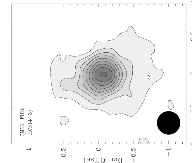
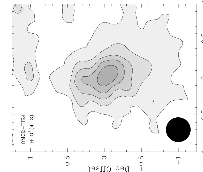
Figure 3: HCN and HCO⁺ ($J\rightarrow 4-3$) maps of OMC2-FIR4. Although the ion spatial distribution appears somewhat more extended, the two peaks are well aligned and the HCN and HCO⁺ systematic velocities agree (from figure 2). The two maps have the same lowest contour level of 5 K$\cdot$km/s ($\sim 10\sigma$) and the following levels increase linearly with an interval of 5 K$\cdot$km/s. The maps’ grid spacing of $10\arcsec$ is half of the beam width (shown in the lower left corners). The pointing accuracy is better than $\sim 5\arcsec$.

We present in figure 2 spectra of these three molecules in the $J\rightarrow 3-2$ transition for OMC1 and $J\rightarrow 4-3$ for OMC2-FIR4, OMC3-MMS6 and DR21OH obtained at the Caltech Submillimeter Observatory with the 200-300 GHz and 300-400 GHz receivers. The observations (including the maps presented in figure 3) were done on several nights during the months of March, April, June and August 1999. Pointing was checked at regular interval using scans made on planets available at the time. Telescope efficiencies were calculated to be $\sim 70$ % for the 200-300 GHz receiver (beam width of $\sim 32\arcsec$) and $\sim 60$ % for the 300-400 GHz receiver (beam width of $\sim 20\arcsec$).

As can be seen from figure 2, all these spectra show the characteristics described earlier; the ion lines are all significantly narrower than the HCN lines and the suppression of the wings is also obvious. These conclusions are made more definite in table 2 where we present a comparison of the line widths (more precisely the standard deviations $\sigma_{v}$) of the species for these molecular clouds. The widths were measured after the lines were modeled with a multi-Gaussian profile. We interpret the fact that the predictions made here on the differences in the appearance in the spectra between comparable neutral and ion molecular species seem to be easily observable in molecular clouds as strong evidence in favor of our assertions.

We should however point out that the differences between the line profiles of neutral and ion species could be partly due to other factors. Indeed, the assumed coexistence of the different molecular species is not necessarily correct. Although we tried to choose ion and neutral species that are as similar as possible, it is likely that their observations sample different parts of the molecular clouds. In some cases, it might even be possible that two species are exposed to significantly different dynamical processes that could cause one of them to exhibit a narrower or larger line profile no matter what the effect of the magnetic field might be. Maps of the different molecular species for a given object could shed some light on this question. In the case of OMC1, Ungerechts et al. (1997) have extensively mapped the Orion molecular cloud (around OMC1) with 20 different chemical and isotopic molecular species. Amongst other things, they find an impressive degree of uniformity in the chemical abundances; but most interesting to us is how similar their maps of HCN and HCO⁺ are ($J\rightarrow 1-0$, beam width of $\sim 50\arcsec$). On the other hand, N₂H⁺ seems to have a very different spatial distribution (see their figure 2). We also present in figure 3 our maps of OMC2-FIR4 in HCN and HCO⁺ ($J\rightarrow 4-3$) done at the CSO. Although the ion species appears somewhat more extended, the two peaks are well aligned. This and the fact the two species have similar line center velocity (see figure 2) brings support to the coexistence assumption for these molecules in the OMC2 cloud.

The question of abundances is also important. For example, a given species could exhibit more opaque lines which could change some characteristics of the line profiles (such as the relative importance of the high velocity wings, saturation or self-absorption). In fact, we believe that the differences between the spectra of N₂H⁺ and HCO⁺ are probably the result of this effect (see the case of DR21OH in figure 2, the self-absorption feature at $\sim-2.5$ km/s is much weaker in the N₂H⁺ spectrum implying a lower abundance).

Chemical differentiation could also play a role in explaining the differences between spectra. In this effect, we expect that our analysis only applies to long-lived ion species (like the protonated molecules considered here), other more reactive species (CO⁺, SO⁺, …) should more or less behave as neutrals as almost every collision in which they are involved would entail a chemical reaction (Schilke, 1999).

4 Relaxation time and interaction between charged particles.

In our analysis of the problem in section 2, we have considered the behavior of a given ion without taking into account the presence of any other charged particles. One might intuitively guess that for a weakly ionized plasma, like the ones probed with our observations at the CSO presented in the last section, it is probably safe to do so.

One can make sure of this by comparing the mean time between collisions for charged particles in such a plasma with the time it takes an ion to relax to its steady state after being excited to a different velocity. The excitation could occur, for example, during a collision with an electron. However, because of the huge disparity between the masses of the two particles, it is unlikely that the ion would be much perturbed by such an encounter. A collision with another ion is more likely to produce a significant change in its velocity.

At any rate, it turns out that the ion relaxation time is given by the reciprocal of the relaxation rate defined by equation (15), as one can verify when solving the equation of motion (1) for a mean collision force $\left\langle\mathbf{F}_{c}\right\rangle$. The solution shows that the ion velocity decays exponentially with a time constant equal to $\left\langle\omega_{r}\right\rangle^{-1}$. When this time is compared to the mean collision time between ions, it is seen to be at least a few orders of magnitude smaller. Our simplified analysis is therefore justified.

5 Conclusion.

We argue that the presence of a magnetic field in a weakly ionized plasma can be easily detected through a comparison of ion and neutral line profiles. More precisely, we expect ion lines to often exhibit narrower profiles and significant suppression of high velocity wings. We have presented observational evidence obtained for four different molecular clouds which agrees with our theory.

Because of the low intensities of field required for the effect to be noticeable, we expect the phenomenon to be widespread. However, where the mean magnetic field is aligned with the neutral flow(s), or where the line width is dominated by the thermal width, should not show any significant differences between comparable neutral and ion spectra. These aspects of the problem will be treated in subsequent papers.

Appendix A Derivations.

Equations (3) and (4) can be easily derived by taking the mean of the equation of motion (1) and then assuming a steady state:

$$\left\langle\frac{d\mathbf{v}}{dt}\right\rangle=0$$

Using equation (2) as an approximation for the force of interaction between ions and neutrals we get from the mean equation of motion:

$$\left\langle\mathbf{F}_{c\|}\right\rangle = 0$$ (A1)

$$\left\langle\mathbf{F}_{c\bot}\right\rangle = -\frac{e}{m_{i}c}\left\langle\mathbf{v}_{\bot}\right\rangle\times\left\langle\mathbf{B}\right\rangle$$ (A2)

with

$$\left\langle\mathbf{F}_{c}\right\rangle=-2\frac{\mu}{m_{i}}\nu_{c}\left(\left\langle\mathbf{v}\right\rangle-\left\langle\mathbf{v}^{n}\right\rangle\right)$$ (A3)

where $\nu_{c}$ is the mean collision rate. From equation (A1) and (A3) it is straightforward to get equation (3) for $\left\langle\mathbf{v}_{\|}\right\rangle$. Equation (A2) can be transformed to:

$$\left\langle\mathbf{v}_{\bot}\right\rangle=-\frac{\left\langle\omega_{r}\right\rangle}{\left\langle\overrightarrow{\omega_{g}}\right\rangle^{2}}\left[\left(\left\langle\mathbf{v}_{\bot}\right\rangle-\left\langle\mathbf{v}_{\bot}^{n}\right\rangle\right)\times\left\langle\overrightarrow{\omega_{g}}\right\rangle\right]$$

into which we can insert equation (A2) using (A3) and finally get equation (4) which we rewrite here:

$$\left\langle\mathbf{v}_{\bot}\right\rangle=\frac{\left\langle\mathbf{v}_{\bot}^{n}\right\rangle+\left\langle\omega_{r}\right\rangle^{-1}\left[\left\langle\mathbf{v}_{\bot}^{n}\right\rangle\times\left\langle\overrightarrow{\omega_{g}}\right\rangle\right]}{1+\left(\frac{\left\langle\overrightarrow{\omega_{g}}\right\rangle}{\left\langle\omega_{r}\right\rangle}\right)^{2}}$$ (A4)

$\left\langle\overrightarrow{\omega_{g}}\right\rangle$ and $\left\langle\omega_{r}\right\rangle$ are defined in equation (8) and (9) respectively.

Equations (5) and (6) for the velocity dispersions can be derived by using the following procedure. We concentrate on the equation for $\sigma_{\bot}^{2}$. If we assume that the time of interaction during a collision is infinitively small, we can express $\mathbf{v}_{\bot}^{\prime}$, the ion velocity (perpendicular to the field) immediately after a collision, as a function of the velocity $\mathbf{v}_{\bot}$ just before the collision:

$$\mathbf{v}_{\bot}^{\prime}=\mathbf{v}_{\bot}+\frac{\Delta\mathbf{p}_{\bot}}{m_{i}}$$ (A5)

with $\Delta\mathbf{p}_{\bot}=-2\mu\left(\mathbf{v}_{\bot}-\mathbf{v}_{\bot}^{n}\right)$ the change in the ion momentum. Upon taking the mean of the square of equation (A5) while once again imposing steady state conditions, i.e. $\left\langle\left|\mathbf{v}_{\bot}^{\prime}\right|^{2}\right\rangle=\left\langle\left|\mathbf{v}_{\bot}\right|^{2}\right\rangle$, we are left with:

$$\left\langle\mathbf{v}_{\bot}\cdot\frac{\Delta\mathbf{p}_{\bot}}{m_{i}}\right\rangle=-\frac{1}{2}\left\langle\left|\frac{\Delta\mathbf{p}_{\bot}}{m_{i}}\right|^{2}\right\rangle$$ (A6)

Taking into account the fact that $\left\langle\mathbf{v}_{\bot}\right\rangle\cdot\left\langle\mathbf{v}_{\bot}^{n}\right\rangle=\left\langle\mathbf{v}_{\bot}\right\rangle^{2}$, as can be verified with equation (A4), it is then straightforward to obtain:

$$\sigma_{\bot}^{2}=\frac{\left\langle\left|\mathbf{v}_{\bot}^{n}\right|^{2}\right\rangle-\left\langle\mathbf{v}_{\bot}\right\rangle^{2}}{\left[\frac{m_{i}}{\mu}-1\right]}$$ (A7)

The equation for $\sigma_{\|}^{2}$ follows from the same procedure.

The more refined set of equations (10)-(15) can also be obtained in similar fashion but the task is rendered somewhat more complicated by the fact the interaction force $\mathbf{F}_{c}$ is not simply given by equation (2). We will omit their derivation here as they are somewhat lengthy and don’t bring anything substantially new to the discussion.

One last word concerning the energetics involved in the collision process. From the above discussion, it is apparent that an ion which starts off with the same velocity as the neutral flow would eventually settle into a steady state of lower kinetic energy (assuming a strong magnetic field). Once again focusing on the approximate head-on collision model as seen in the reference frame of the observer, we can understand this loss of energy by noting that the drag force felt by the ion (equation (2)) is proportional to the relative velocity between the colliding particles. As the ion is attempting to travel in a circular orbit around a given guiding center, this relative velocity is greater when it is going upstream (and losing energy through collisions) than when it is going downstream (and gaining energy from the collisions). This will lead, on average, to a net loss of energy over a complete orbit.

Figure 1: Ion effective velocity ($\sqrt{\left\langle\mathbf{v}_{\|}^{2}\right\rangle}$, $\sqrt{\left\langle\mathbf{v}_{\bot}^{2}\right\rangle}$ and $\sqrt{\left\langle\mathbf{v}^{2}\right\rangle}$) as a function of the mean magnetic field strength when $\mathbf{v}_{\|}^{n}=0$, $\left|\mathbf{v}_{\bot}^{n}\right|=10$ km/s, $n=5\times 10^{6}$ cm^-3 and $A_{i}=29$.

Figure 2: HCN (top), HCO⁺(middle) and N₂H⁺ (bottom) observations at the position of peak intensity of (clockwise starting from top left): OMC1, OMC2-FIR4, OMC3-MMS6 and DR21OH. The bump at $\sim 30$ km/s in the middle spectrum of OMC1 is a contamination from other species (SO₂, ¹³CH₃CN, …).

Parameter	$A_{i}=29$	$A_{1}=45$
$\left\langle a\cos\left(\gamma\right)\right\rangle$	0.07734	0.05028
$\left\langle a^{2}\cos^{2}\left(\gamma\right)\right\rangle$	0.00778	0.00332
$\left\langle a^{2}\sin^{2}\left(\gamma\right)\right\rangle$	0.00359	0.00157
$\left\langle a^{2}\right\rangle$	0.01137	0.00489

Table 1: Numerical values for the different averages present in equations (10)-(15) for ion molecular masses of 29 and 45.

	Coordinates (1950)		$\sigma_{v}$(km/s)
Object	R.A.	Decl.	HCN	HCO+	N2H+
OMC-1	5 32 47.2	-05 24 25.3	17.42	3.23	1.87
OMC-2 FIR 4	5 32 59.0	-05 11 54.0	3.59	2.72	1.34
OMC-3 MMS 6	5 32 55.6	-05 03 25.0	1.40	0.71	0.56
DR 21(OH)	20 37 13.0	42 12 00.0	5.75	4.61	2.08

Table 2: Comparisons of line widths (standard deviations $\sigma_{v}$) between HCN, HCO⁺, and N₂H⁺ for the four objects presented in figure 2.

References

- Choudhuri (1998) Choudhuri, A. R. 1998, The physics of fluids and plasmas, an introduction for astrophysicists (Cambridge)
- Crutcher et al. (1993) Crutcher, R. M., Troland, T. H., Goodman, A. A., Heiles, C., Kaz s, I., & Myers, P. C. 1993, ApJ, 407, 175
- Crutcher et al. (1999) Crutcher, R. M., Troland, T. H., Lazareff, B., Paubert, G., Kaz s, I. 1999, ApJ, 514, L121
- Draine & Weingartner (1996) Draine, B. T., & Weingartner, J. C. 1996, ApJ, 470, 551
- Falgarone & Phillips (1990) Falgarone, E. & Phillips. T. G. 1990, ApJ, 359, 344
- Hildebrand et al. (1999) Hildebrand, R. H., Dotson, J. L., Dowell, C. D., Schleuning, D. A., & Vaillancourt, J. E. 1999, ApJ, 516, 834
- Mouschovias (1991a) Mouschovias, T. Ch. 1991a, in The physics of star formation, eds. C. J. Lada, N. D. Kylafis (Dordrecht: Kluwer), 61
- Mouschovias (1991b) Mouschovias, T. Ch. 1991b, in The physics of star formation, eds. C. J. Lada, N. D. Kylafis (Dordrecht: Kluwer), 449
- Schilke (1999) Schilke, P. 1999, private communication
- Shu et al. (1987) Shu, F. H., Adams, F. C., & Lizano, S. 1987 ARA&A, 25 ,23
- Tennekes & Lumley (1972) Tennekes, H & Lumley, J.L. 1972, A first course in Turbulence (MIT Press)
- Ungerechts et al. (1997) Ungerechts, H., Bergin, E. A., Goldsmith, P. F., Irvine, W. M., Schloerb, F. P., & Snell, R. L. 1997, ApJ, 482, 245.
- Zuckerman & Evans (1974) Zuckerman, B., Evans, N. J. II 1974, ApJ, 192, L149.