The H$\alpha$ Light Curves and Spatial Distribution of Novae in M81

Abstract

We present the results of a preliminary H$\alpha$ survey of M81 for novae conducted over a 5 month interval using the 5’ field of view camera (WFCAM) on the Calypso Telescope at Kitt Peak, AZ. We observed M81 nearly every clear night during this interval, covering the entire galaxy, and discovered 12 novae. Our comprehensive time coverage allowed us to produce the most complete set of H$\alpha$ light curves for novae in M81 to date. A raw nova rate for M81 gives 23 yr^-1 which, because of the nature of our survey, is a hard lower limit. An analysis of the completeness in our survey gives a corrected nova rate of 30 yr^-1. This agrees well with the rate of 33${}^{+13}_{-8}$ yr^-1, derived from Monte Carlo simulations using nova light curves and survey frame limits. The spatial distribution of the novae we discovered follows the bulge light much better than the disk or total light according to Kolmogorov - Smirnov tests of their radial distributions. The asymmetry in the distribution of novae across the major axis line of M81 implies a bulge-to-disk nova ratio of $>$ 9 and supports the idea that novae originate primarily in older stellar populations.

1 Introduction

Extragalactic novae are particularly appealing objects for studies of close binary evolution. They are the tracer of interacting close binary stars, visible to much greater distances than any other well studied standard candle except supernovae (novae display M_v up to $-10$). By studying the novae in a nearby galaxy, one can gather a homogeneous sample of objects, all at the same distance, that is not plagued by the selection effects hampering an analysis of the cataclysmic variable (CV) population in our own galaxy.

Given the large fraction of all stars that exist in binaries, the effort to understand binary formation and evolution has wide reaching implications for understanding stellar populations. There are currently many unsolved problems in the theory of close binary formation and evolution that are difficult to tackle using CVs in our own galaxy because of the selection effects mentioned above.

The prediction that the nova rate should correlate with the star formation history in the underlying stellar population (Yungelson, Livio, & Tutukov, 1997) is one example. This prediction is based on our understanding of how close binaries form and evolve, combined with our understanding of how the mass of a nova progenitor influences the nova outburst. Massive white dwarfs come from massive progenitors. These massive white dwarfs erupt as novae frequently as they need only accrete a small amount of hydrogen from their companions to explode as novae. This, in turn, implies that stellar populations with a low star formation rate should have a correspondingly low nova rate, i.e., early-type galaxies with older stellar populations should have a lower luminosity specific nova rate (LSNR) than late-type galaxies with ongoing star formation.

Efforts have been made to detect a trend in LSNR with galaxy type (della Valle et al., 1994; Shafter, Ciardullo, & Pritchet, 2000), but the random errors are too large to date for a meaningful comparison. Typical extragalactic nova surveys are carried out using short runs, and significant assumptions must be made about the mean lifetimes of novae in order to derive nova rates (Shafter & Irby, 2001). It is also rare that an extragalactic survey has been able to spatially cover an entire galaxy and avoid making some assumption about the distribution of novae with light to derive a galactic nova rate. The resulting errors in the nova rates are large, but systematic biases are far more pernicious.

In order to accurately compare nova rates with the underlying stellar population, we are pursuing a research program that uses the comprehensive time and spatial coverage afforded by a dedicated observatory. We have begun our program with M81 and used 5 continuous months of observing time to produce a survey that requires no assumptions about nova distribution or mean lifetime. Not since Arp (1956) surveyed the central parts of M31 has such extensive, continuous coverage of a galaxy for novae been attempted.

Our survey updates the 5 year photographic survey of M81 for novae reported by Shara, Sandage, & Zurek (1999). They found 23 novae, evenly divided over the disk and central bulge. Significant incompleteness must be present in that survey due to photographic saturation in the bright central regions of the galaxy and due to large gaps in their time coverage. The results we present below show that a comprehensive spatial and temporal survey is required to minimize the systematic effects of incompleteness.

2 Observations

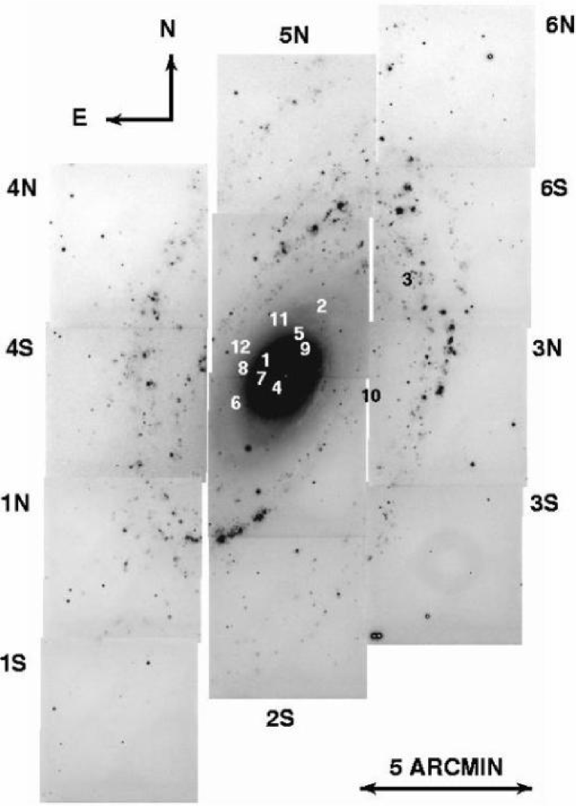
Figure 1: H$\alpha$ mosaic of the 12 M81 survey fields (labeled) with the positions of the 12 novae discovered in the 2003 season indicated as white or black numbers. Note that most of the novae are close to the nucleus of the galaxy and the asymmetry of the nova distribution across the major axis.

We used the WFCAM 2048x2048 pixel CCD on the Calypso 1.2m telescope at 4x4 binning for our observations of M81. This configuration yields a pixel scale of 0”.6 px^-1 and a field size of 5’ on a side. The seeing for our observations had a median of 1”.5 and ranged from 1”.0 to 2”.5. In an effort to cover the entire spatial extent of M81 in our search for novae we divided M81 into 12 fields covering roughly 15’ in Right Ascension and 23’ in Declination. Figure 1 is an H$\alpha$ mosaic of the 12 fields showing the extent of our spatial coverage, the identification of the fields, and the location of the 12 novae discovered.

All observations were taken through an H$\alpha$ filter with a 30Å full width at half-maximum (FWHM) bandpass. This filter was chosen for several reasons. Because of the longer duration of novae in H$\alpha$ compared to the B-band (Ciardullo et al., 1987), we minimize the possibility of missing novae due to inevitable gaps in coverage. The redder wavelengths observed with the H$\alpha$ filter means that our images are less influenced by internal extinction in M81, and less influenced by scattered moonlight during the fuller phases of the moon. To illustrate this point, Figure 2 shows the distribution of frame limits (described in § 4) with days from New Moon. Only within 1.5 days of the full moon is any effect seen. It is also our goal to explore the H$\alpha$ light curve as a tool for understanding the physics of nova outbursts. So far attempts to do this have failed, but with our dense time sampling the possibility opens up that features of the H$\alpha$ rise, previously poorly observed, may correlate with properties of the nova progenitor.

Each individual exposure was 1200s and we attempted to get at least 5 exposures on a given field in one night for a total exposure time of 100 minutes per epoch. Although most of our epochs reached this goal, observing conditions varied considerably and so the number of useful exposures per epoch ranges from 2 to 9.

Ideally we would have observed all 12 fields every clear night. This was impossible to achieve with the requirement that we get 100 minutes of exposure per epoch. Thus, we cycled through the 12 fields over the course of a varying number of nights depending on the time available on a given night subject to weather, M81’s availability, and occasional equipment problems. Guide stars were not readily available for some of the fields or were faint, with the result that the number of usable survey epochs for each field varies from 5 to 21.

Our survey ran from December 31, 2002 (JD 2452638.8) to June 6, 2003 (JD 2452796.6) covering a total of 158.8 days. At the end of this time, two novae were still observable in decline in one of the fields (5S). An additional 15 epochs were obtained of this field to follow the declining novae until June 26, 2003 (JD 2452816.7), during which time no new novae were discovered in this field. This period from June 6 to June 26, 2003 is not included in our nova rate calculations.

Table 1 summarizes the observations in our survey. The field designations correspond to those in Figure 1, with the exception that field 5S and 2N are unlabeled (but their location is obvious). The fields with Bulge in the last column also contain a significant amount of M81’s disk as can be seen from Figure 1.

3 Reduction

All exposures were bias subtracted and flat fielded using the standard tools in IRAF (Tody, 1986). The exposures for a given epoch (from 2 to 9) were then registered and combined to produce a coadded image for each epoch using the following DAOPHOT programs (Stetson, 1987): DAOPHOT to measure the point sources, DAOMATCH and DAOMASTER to derive and refine the transformations, and MONTAGE2 to perform the registration and coaddition. The registration master was chosen to be the best coadded image from the entire set for a given field based on measurements of the seeing in each coadded image over the entire survey. The coaddition process removed all but a few cosmic rays.

4 Nova Detection

The coadded images were blinked against each other to detect changing point sources. Nova candidates were required to be observed in at least two epochs and to be missing on an epoch of sufficient depth coverage to confirm its transient nature. We also used the raw images for an epoch to confirm the presence of the candidate in each individual frame.

For the bulge region of M81 (Fields 2N and 5S), where the intensity gradient makes detection more difficult, we used the following technique. We produced a spatial median filtered image of the coadded frame using a box size of 11 by 11 pixels to remove point sources and preserve the low frequency structure of the image. This was then subtracted from the original coadded frame which removed the intensity gradient of the bulge, but preserved the point sources embedded within it. Residual light in the subtracted image within 20” of the nucleus made detection of the innermost novae very difficult. This subtraction technique was performed on each coadded image of the bulge fields after which they were blinked against each other. Since most of the novae were detected in the bulge region, the subtraction proved to be important for detecting novae in M81.

For each coadded image of each field we determined the frame limit by using artificial stars and the exact techniques outlined above for detecting the novae. Closer to the nucleus of M81, frame limits were derived from the flattened images. For field 2N, an additional set of frame limits was derived near the position of Nova 4. For field 5S, two additional sets of frame limits were derived near the positions of Nova 1 and Nova 5.

Table 2 summarizes the 12 novae discovered with our survey. Astrometry was derived for each nova using the WCSTOOLS package (Mink, 2002) and the Guide Star Catalog-II. Positions are accurate to better than 2” based on the fit residuals to the GSC-II stars. The corrected nuclear distances were calculated using the equations and parameters given in Shara, Sandage, & Zurek (1999).

Could our candidates be anything other than novae? Their positions in M81 rule out foreground or background objects. We checked the position of each candidate against the list of known Hubble-Sandage (HS) variables in M81 (Sandage, 1984) and found no coincidence. These bright blue HS variables are the only known non-nova variables that approach the brightnesses of our candidates. In fact, the brightest B-band magnitude for the HS variables in M81 is 19.1 (Sandage, 1984). These are massive stars and are likely to be much fainter in the red at the H$\alpha$ passband than in the B-band. Considering the peak magnitudes of our candidates (see below), there is little chance that any of our nova candidates is actually one of these bright blue variables…or anything other than a nova.

5 Nova Photometry

Since crowding was not an issue, aperture photometry was used to measure point source brightnesses in each coadded image. We used the IRAF apphot package to measure point source brightnesses. Variable seeing was accounted for by setting the measurement aperture radius in each image to 1/2 the FWHM of the stellar profile to maximize the signal-to-noise ratio. The FWHM was measured from a set of well isolated stars in each image.

The photometric calibration was achieved using a two-step process, which was required because of the negligible overlap between fields, and the lack of H$\alpha$ standards in many of the fields. The first step was to tie all the frames to a common system. This was achieved using the R-band photometry of Perelmuter & Racine (1995). An offset from our instrumental H$\alpha$ magnitudes to the calibrated R magnitudes was calculated for each epoch of each field using from 18 to 70 stellar sources per field with an accuracy of better than 0.1 magnitude. Non-stellar sources (HII regions) were excluded by virtue of their much brighter instrumental H$\alpha$ magnitude relative to R than the stellar sources.

Once all magnitudes were on this common R system, an offset was needed to the standard AB system where $m_{H\alpha}=0.0$ for $f_{\lambda}=2.53\times 10^{-9}$ erg cm^-2 s^-1 Å^-1. For our filter with a FWHM of 30Å, this gives a zero point flux of $7.59\times 10^{-8}$ erg cm^-2 s^-1. We used the foreground extinction corrected and standardized flux measurements of M81 planetary nebulae (PNe) published by Magrini et al. (2001) to calculate this offset. They used a 90Å FWHM H$\alpha$ filter which would include [NII] if present. Our filter excludes [NII] so we had to assume that for the set of PNe used, the [NII] fluxes are small. Using our filter zero point flux, we converted the fluxes from Magrini et al. (2001) into H$\alpha$ filter magnitudes for the 107 PNe we were able to measure in 7 of our fields. We then compared these H$\alpha$ filter magnitudes with the common R system magnitudes for the PNe to calculate an offset between the two systems. We calculated a mean offset from 78 PNe of $-0.26\pm 0.13$ magnitudes. We excluded 29 outliers that showed evidence of stronger [NII] by virtue of their having a lower instrumental H$\alpha$ magnitude than predicted from the conversion of the flux to H$\alpha$ filter magnitude. Without individual spectra of the PNe, this exclusion is less than perfect and limited our photometric accuracy.

As a check on this calibration, we found one object which is in both the R catalog of Perelmuter & Racine (1995) and the H$\alpha$ flux catalog of Magrini et al. (2001). Object 2111 from Perelmuter & Racine (1995) with an R magnitude of 19.64 is object 93 from Magrini et al. (2001) which has an H$\alpha$ magnitude (using the zero point flux above) of 19.42. This gives an offset of -0.22, in good agreement with our calibration.

This calibration should allow comparison of our H$\alpha$ nova light curves with the M31 H$\alpha$ light curves of Ciardullo et al. (1990), with one important caveat. Because our filter is 2.5 times narrower, many of the faster novae with expansion velocities $>$ 685 km s^-1 have overfilled our 30Å bandwidth. The M31 novae can have expansion velocities up to 1715 km s^-1 and not overfill the 75Å filter bandwidth used by Ciardullo et al. (1990). Because nova ejection velocity is a function of nova luminosity (Shara, 1981), a direct comparison of the nova luminosity distribution between M31 and M81 is precluded for this survey.

Table 3 presents our calibrated photometry for each nova at each observed epoch. The errors in Column 3 are the 1-$\sigma$ internal photometric errors. The three points in parenthesis for Nova 6 are unfiltered magnitudes from the KAIT telescope (Weisz & Li, 2003). Filippenko & Chornock (2003) report that the spectrum of this nova exhibited strong double-peaked hydrogen Balmer emission lines and that many Fe II, Ca II, and O I lines also appeared in emission, and thereby confirm this object as a nova.

6 The H$\alpha$ Light Curves

Figure 3 and Figure 4 present our calibrated H$\alpha$ light curves for the 12 novae discovered in M81 during our survey. Figure 3 presents the 6 novae for which we have observed the maximum $m_{H\alpha}$, while Figure 4 presents the 6 novae observed days or weeks after maximum $m_{H\alpha}$. The frame limits are plotted as short horizontal lines with downward pointing arrows, while the solid circles with error bars are the nova observations from Table 3.

A simple linear fit was made to the decline portion of each light curve to calculate the decline rates in $m_{H\alpha}$ day^-1. The thin lines in Figure 3 and Figure 4 show the resulting fits. Table 4 presents the properties of the nova light curves including the rise time and decline rate for each nova. We consider the H$\alpha$ rise times to be lower limits because we do not have continuum light curves to to accurately define the outburst time.

We cannot compare the brightness distribution of our novae to that in M31, because of the filter-overfilling described above, but we can compare the nova decline rates. Figure 5 shows the comparison of our decline rates with the M31 decline rates reported in Ciardullo et al. (1990) and Shafter & Irby (2001). We see that the distribution is similar, but there is an indication of incompleteness in our slowest decline rate bin. Both M31 surveys spanned at least two years and therefore had longer overall time baselines. Our survey is continuous, but only covers a 5 month period. At the slowest reported decline rate for an M31 nova of 0.0018 $m_{H\alpha}$ day^-1 (Ciardullo et al., 1990), in 5 months a nova would only change by 0.3 magnitudes in H$\alpha$ and would not be seen in our survey as a transient point source. In fact, it would take over 500 days before such a slow nova would change by one magnitude. Based on Figure 5, and accounting for small number fluctuations, we estimate that there are roughly 10 very slow novae that remain to be detected in the present survey. As we extend our survey in time, we will continue to blink epochs from the season reported here in an effort to discover these very slowly declining novae.

Two of the light curves show that, in H$\alpha$, novae can take a long time to reach maximum brightness; Nova 12 took more than 13 days , and Nova 5 took at least 50 days. Nova 12 can be compared with Nova 26 in Ciardullo et al. (1990) which took $\sim$15 days from outburst to reach maximum. Our Nova 5 is unprecedented; its 50 day rise is, as far as we know, the longest ever observed for a nova in H$\alpha$. Nova 20 from Ciardullo et al. (1990) shows a small decline before reaching maximum light, like our Nova 5, and could have taken a similar length of time to reach maximum.

Figure 6 shows a comparison of nova rise times in H$\alpha$ and the continuum. The H$\alpha$ data consist of the 6 novae from this paper (see Table 4) and the three novae with well observed rises from Ciardullo et al. (1990). The continuum data are from the photographic light curves presented in Arp (1956). Of the 30 novae discovered by Arp, we used 21 for which we could determine a reliable rise time. The continuum distribution has a sharp peak at 1 day, but extends out to nearly as long a rise time as the longest one for H$\alpha$. The H$\alpha$ distribution shows no peak, and does seem to cluster in the range from 3 to 15 days. The arithmetic mean of the continuum rise times is 9.0 days. The arithmetic mean for the H$\alpha$ rise times is 13.3 days, but should only be considered a lower limit given that all the rise times from Table 4 are lower limits. For the four novae from Ciardullo et al. (1990) that have both B-band and H$\alpha$ photometry (including Nova Cyg 1975), we see that the H$\alpha$ maximum always occurs after the B-band maximum. It appears that H$\alpha$ rise times are generally longer than continuum rise times, but without a large set of light curves in both continuum and H$\alpha$ for each nova, we cannot say more. We hope to remedy this in the next observing season for M81 (see below).

The slow rise times in H$\alpha$ of some novae may lead to inaccuracy in the calculation of nova rates if only the maximum light and decline rates are used, especially with a survey, such as ours, with many closely spaced epochs. Nova light curves which cover the rising portion of the outburst and allow determination of the decline rate are needed for calculating accurate completenesses and nova rates.

7 Completeness

Because of the dense time sampling and variable depth of our survey, we developed an approach to finding the completeness of each field that is more appropriate than assigning a single frame limit to the entire survey. With a set of relatively complete H$\alpha$ nova light curves and the frame limit for each epoch of each field, we can calculate the completeness for a given field by simulating the random outburst times of a large sample ($10^{5}$) of novae. This approach assumes that we have a set of H$\alpha$ light curves that is representative of the nova population in M81.

7.1 Representative H$\alpha$ Light Curves

Of the 12 light curves reported in this work, three novae have sufficient coverage of the rising part of the light curve and have reasonably well determined decline rates to qualify for this set: Novae 5, 7, and 12 (see Figure 3). We can combine these with the H$\alpha$ photometry of the 8 novae listed in Table 11 of Shafter & Irby (2001) to get a representative set of 11 H$\alpha$ nova light curves to use in our random outburst simulation.

In order to include the M31 light curves in our representative set, we need to correct for the difference in galaxy distances and the difference in filter bandwidths. Using the distance moduli quoted in Shafter, Ciardullo, & Pritchet (2000) we apply a correction to the M31 novae of +3.48 magnitudes to place them at the distance of M81. The filter bandpass we used is 2.5 times narrower than used by Ciardullo et al. (1990) for the M31 novae and so they would appear 1 magnitude brighter in our survey making the correction +2.48 magnitudes. If the M31 novae had, in fact, been observed with our filter, they would have overfilled the bandpass by varying amounts and therefore been fainter by up to a factor of 2. Spectroscopic observations of M31 novae by Ciardullo, Ford, & Jacoby (1983) show typical emission line widths of 40-60 Å. However, spectra of novae in M31 reported by Tomaney & Shafter (1992) show the slowest, and therefore faintest, novae to have expansion velocities of less than 685 km s^-1, which would not overfill our filter. Since we are interested in calculating the completeness at the faint end, we elect not to apply an uncertain overfilling factor to the M31 novae. Therefore, our total correction to the M31 novae to include them with our M81 photometry through a 30 Å filter is +2.48 magnitudes.

To see if this set is truly representative of novae in M81, we can compare the range of decline rates in this set (0.0044 to 0.087 mag day^-1) with Figure 5. We see that this range covers the majority of the novae in this figure. By adding the slower novae from M31, we account for the very slow novae we are apparently missing, according to Figure 5. We can also compare the range of maximum magnitudes in this set ($m_{H\alpha}$ from 17.0 to 20.9) with the maximum magnitudes reported in Ciardullo et al. (1990) for M31. After accounting for the magnitude offset as described above, we see that our set spans the majority of the range of novae in M31. For the following analysis, we will assume that our 11 novae are a representative set for M81.

7.2 Random Outburst Simulations

We used each nova in this representative set to make a random outburst simulation for each set of frame limits we measured. This produced 11 simulations for each of the 15 frame limit sets for a total of 165 simulations. To create each simulation, which consisted of 10⁵ trials, we used an uniformly distributed random number generator to shift the representative nova light curve in time so that its outburst occurred within the 159 days of our survey. The frame limit set being studied was then compared with each shifted light curve to determine if it would have been a valid nova candidate in that field. A valid candidate must pass the criteria describe above: it must be brighter than at least two frame limits in the set, and it must be fainter than at least one of the frame limits, to confirm its transient nature. The number of times a simulated nova was identified as a candidate was divided by the number of trials to produce a fractional completeness for that representative nova in the frame limit set being studied.

In order to compare the randomly shifted nova light curve with the frame limits in the set, and determine if the simulated nova would have been a candidate in the field being studied, the following algorithm was adopted. Any nova magnitude on a frame epoch before outburst was set to 99.9 (i.e. a non-detection). Nova magnitudes on frame epochs between two light curve points were calculated using linear interpolation. Nova magnitudes on frame epochs after the last point in the light curve were calculated using the measured decline rate for the nova. This is much more accurate than extrapolating beyond the end of the light curve since the last points in a nova light curve tend to be the faintest and therefore the noisiest.

The completeness as a percentage, averaged over the 11 representative novae, is given for the 15 frame limit sets in Table 5 and plotted in Figure 7. Two correlations are apparent. The first and strongest is the correlation with the number of observed epochs. The lowest completeness is obtained for the fields with the smallest number of observed epochs and suggests a substantial incompleteness for these fields. The other correlation is with nuclear distance. For fields 2N and 5S, the completeness drops considerably as the distance to the nucleus decreases. For a frame limit set measured at 42” from the nucleus of M81, and plotted in Figure 7 as a filled diamond, we derive a completeness of 72%. For the closest frame limit set at 24” from the nucleus, and plotted in Figure 7 as a filled square, we derive a completeness of only 48%. This suggests that a significant incompleteness exists in our survey within an arcminute of the nucleus of M81.

The completeness as a percentage, averaged over the 15 frame limit sets, is given for the 11 representative novae in Table 6 and plotted in Figure 8. The effect of maximum magnitude on completeness is readily apparent. This trend is not without scatter, however, due to the complex interaction between the shape of the light curve and the depth of the survey as a function of epoch.

8 The Nova Rate

The effects noted above demonstrate that assigning a single limiting magnitude to our survey is overly simplistic. This fact, combined with our dense time coverage, indicates that we can improve on the mean nova lifetime approach of Ciardullo et al. (1990) for calculating the nova rate for M81. A raw global nova rate can be obtained simply by dividing the observed number of novae that erupted during the survey by the time covered. Excluding the two novae that erupted before the start of the survey (Nova 1 and Nova 3) gives $R=10/0.43$yr $=23$ yr^-1 and is obviously a hard lower limit on the M81 nova rate. This rate also requires no correction for partial spatial coverage since we are covering the entire galaxy. For comparison, Shafter, Ciardullo, & Pritchet (2000) report a nova rate for M81 of $R=24\pm 8$ yr^-1, based on 15 novae discovered over a three year period, and refer to an unpublished study whose preliminary results indicate that the nova rate in M81 may be somewhat lower than this.

We can adjust our raw rate by the completenesses shown in Table 5. Since the novae in fields 2N and 5S were distributed closer to the nucleus of M81, we must account for the lower completenesses found. For field 2N, we use a completeness which is the average of the two positions measured, or 64%. For field 5S, we also average the completeness measurements to get a 82% average completeness. Dividing the number of novae that erupted in each field by the appropriate completeness fraction and adding, we derive a completeness corrected number of novae during our 5 month survey of 13. Using this corrected number of novae, we find a global M81 nova rate of $R=13/0.43$yr $=30$ yr^-1. This is still a conservative lower limit because by averaging the completenesses in the two Bulge fields, we are assuming that the number of novae at each measurement location is the same. Figure 1 shows that the novae are more likely to come from the regions of lower completeness nearer to the nucleus of M81 and hence the true completeness correction is probably larger than what we have used here.

8.1 The Monte Carlo Approach

Shafter & Irby (2001) describe a Monte Carlo technique which uses the maximum magnitudes and decline rates of the novae in their Table 11 and their survey faint limit to find the most probable nova rate in their survey region. We used the 11 representative nova light curves described above combined with our frame limits in a similar Monte Carlo experiment to derive nova rates for each of our fields.

This technique makes many independent estimates of the observed nova rate in the given field as a function of the true nova rate $[N_{obs}(N_{t})]$. For a given trial estimate of $N_{t}$, the true rate, we choose a random set of light curves and outburst times and use the frame limits to calculate the number of observed novae, using the candidate criteria described above. We repeat this 10⁵ times and record how many times we recover the number of nova candidates actually observed for that field. The estimate of the true nova rate $N_{t}$ is then incremented and the process is repeated. This produces a probability distribution for $N_{t}$ in the given field. The best estimate for $N_{t}$ is that which corresponds to the peak of this distribution.

Figure 9 shows the probability distributions for an interesting subset of fields. The two distributions at the top of the figure, for Field 1S and Field 4S, show the difference between two disk fields with no observed novae, but very different time coverage and depth. This is reflected in the widths of the distributions and consequently the errors on the estimated true nova rate. The middle two distributions are for fields 3N and 6S, having one nova observed in each. The bottom two distributions are for the two fields that had the bulk of the observed novae with 3 for Field 2N and 7 for Field 5S.

Table 7 presents the results of the simulations for each of 15 sets of frame limits. To derive a global nova rate from these data, we add up the nova rates in all the fields. Without accounting for the incompleteness near the center of M81, i.e., using the frame limit sets derived at the field centers of the two bulge fields, we find a global nova rate of 28${}^{+10}_{-4}$ yr^-1 which is in good agreement with our corrected nova rate of 30 yr^-1. If we include the rates from the frame limit sets closer to the nucleus of M81, as we did for the completeness, we get a higher nova rate. Averaging the two rates for Field 2N we get a rate of 11${}^{+7}_{-5}$ yr^-1. Averaging the three rates for Field 5S we get 18${}^{+7}_{-6}$ yr^-1. Adding these rates to the nova rates for the other fields, we derive a Monte Carlo, completeness-corrected nova rate for M81 of 33${}^{+13}_{-8}$ yr^-1. We point out again that this is a conservative estimate because we have not accounted for the distribution of novae in our simplistic averaging of nova rates for fields 2N and 5S.

8.2 The Luminosity Specific Nova Rate

The 2-micron All Sky Survey (2MASS) offers a uniform infrared photometric system for normalizing nova rates from different galaxies to their underlying stellar luminosity. This will remove one of the major uncertainties in the study of how the luminosity specific nova rate (LSNR) in a galaxy varies with Hubble type. The Large Galaxy Atlas of the 2MASS (Jarrett et al., 2003) gives a K-band integrated magnitude for M81 of 3.831$\pm$0.018. Using this we derive a K-band luminosity for M81 of $L_{K}=8.34\pm 0.14\times 10^{10}L_{\odot,K}$. We derive a LSNR of $\rho_{k}=3.96^{+1.8}_{-1.1}$ yr${}^{-1}[10^{10}L_{\odot,K}]^{-1}$ from our nova rate of 33${}^{+13}_{-8}$ yr^-1, from the Monte Carlo experiment.

This LSNR moves the position of the data point for M81 in Figure 6 from Shafter, Ciardullo, & Pritchet (2000) up from $\rho_{k}=1.80\pm 0.71$. This does not change the conclusion they drew from it, namely that no correlation exists between $\rho_{k}$ and galaxy $B-K$ color. There are many systematic and random errors that could mask such a correlation. The normalization of nova rate to infrared luminosity using 2MASS should reduce the scatter in this diagram caused by non-uniform infrared galaxy magnitudes. We maintain that the biggest source of error in this diagram is that nova rates are systematically underestimated for the inner regions of galaxies where most of the novae may well occur. This figure could change substantially as global nova rates are improved and normalized to a uniform measurement of stellar luminosity for these galaxies. We now show that novae probably do appear preferentially in the bulge of M81.

9 The Spatial Distribution

We do not yet have enough novae in M81 to perform a reliable maximum likelihood decomposition of bulge and disk novae as did Ciardullo et al. (1987) for M31. We can, however, do a simple test comparing the distribution of light and novae. We used the bulge/disk decomposition of Simien & de Vaucouleurs (1986), Table 4, to calculate the cumulative radial distributions of the bulge, the disk, and the total light of M81. We then compared these with the cumulative radial distribution of the novae. We used the Kolmogorov - Smirnov (KS) test to determine at what confidence level we can rule out the hypotheses that the nova distribution is identical to the three different light distributions. Figure 10 shows the results of this comparison.

The ”best match” with the nova distribution of the three is the bulge light distribution which can only be ruled out at the 21% confidence level. The total light fares considerably worse by over a factor of two and can be ruled out at the 57% confidence level. The disk light distribution is the worst match and can be ruled out at the 99% confidence level. Even though the bulge light does the best, the confidence level of 21% is still high. This is most likely due to the incompleteness in the central regions of the galaxy (see Figure 7).

Another diagnostic for the bulge-to-disk ratio of novae was described in Hatano et al. (1997). They used a model for dust in M31 and predicted its effect on the distribution of novae in the bulge region. They state that if novae arise primarily in the bulge, a large asymmetry in their distribution would be apparent because the dust in the disk obscures the bulge novae behind the disk. In this case there would be fewer novae seen on one side of the bulge than on the other. They use the major axis of M31 as the dividing line between novae on top of the disk and novae on the bottom and compared the number of novae below the disk, on the bottom of the bulge, with the number of novae in the bulge above the disk. This ratio is called the bottom-to-top ratio (the BTR). If disk novae predominate, the asymmetry is much less pronounced across this line since the fraction of novae obscured by the disk is the same on each side of the major axis. Using their dust model, Hatano et al. (1997) calculated the BTR for two different scenarios for M31: one with a bulge-to-disk nova ratio of 9 which produced a BTR of 0.33, and one with a bulge-to-disk nova ratio of 1/2 which produced a BTR of 0.63.

If we look at our sample of novae in M81, we can calculate the same BTR diagnostic. M81 clearly has dust in the disk that extends into the bulge (Jacoby et al., 1989). Its inclination of $60^{\circ}\kern-4.83694pt.\kern 0.99585pt4$ (Shara, Sandage, & Zurek, 1999) is not that different from the inclination of $77^{\circ}\kern-4.83694pt.\kern 0.99585pt0$ for M31 (Ciardullo et al., 1987). By examining the image of M81 from the Hubble Atlas (Sandage, 1961), one can see that the top of the bulge is on the north-east side of the major axis line. If we say that the 10 novae within 2’.5 of the nucleus of M81 are the apparent bulge novae, we see that 2 of these novae are south of the major axis line (on the bottom) and 8 of these novae are north of it (on the top) giving a BTR of 2/8 $=$ 0.25. This BTR is much closer to the model for M31 from Hatano et al. (1997) with a bulge-to-disk nova ratio of 9 and clearly rules out the scenario with a bulge-to-disk nova ratio of 1/2. One thing we must consider is that our novae were discovered using H$\alpha$ light, while the models of Hatano et al. (1997) were based on novae in M31 discovered in the B-band. Using the redder H$\alpha$ light should reduce the effect of dust on the discovery rate of novae in the bulge. One would expect, for the same bulge-to-disk nova ratio, that the distribution in H$\alpha$ light would be more symmetric, not less, than the distribution in the B-band. In addition, the fact that M81 is slightly more face on than M31 should also reduce the asymmetry, since a face on galaxy would show no asymmetry regardless of the bulge-to-disk nova ratio. The fact that our distribution is even more asymmetric than their M31 scenario with a bulge-to-disk nova ratio of 9 argues for an even higher bulge-to-disk nova ratio in M81.

Unless the disk of M81 has a vastly different distribution of dust than the disk of M31, one must ask why Hatano et al. (1997) conclude that M31 has a bulge-to-disk nova ratio close to 1/2 while, using the same assumptions, we conclude that M81 has a bulge-to-disk nova ratio greater than 9. One possibility is that Hatano et al. (1997) used data from photographic surveys which have been shown to be incomplete in the inner regions of M31 (Ciardullo et al., 1987). Another problem, compared with our survey, is that M31 has never been surveyed comprehensively. Thus, calculations of the ratio of disk to bulge novae must account for differences in disk and bulge discovery rates from fundamentally different surveys, adding large uncertainties to the calculation. A uniform, comprehensive survey, such as presented here, removes these uncertainties.

The spatial distribution of the novae in M81 adds more weight to the idea that novae are associated with older stellar populations. It is important to continue to test this idea because, if verified beyond a doubt, it would strongly constrain the theory of how these objects form and evolve. We would have to consider that novae take much longer to form than previously thought and may not appear at all in young stellar populations.

10 Bulge versus Disk Novae

We can examine our novae sample in M81 to test the idea that bulge novae are preferentially fainter and slower than disk novae. della Valle & Livio (1998) found that for novae in the Milky Way, the bulge novae were spectroscopically distinct, having Fe II lines in the early emission spectrum, slower expansion velocities, and slower decline rates, while the disk novae had He and N lines, larger expansion velocities, and faster decline rates. Unfortunately, the two unambiguous disk novae reported here, Novae 3 and 10, were not covered well enough to determine their maximum magnitudes, although their decline rates are toward the slow end of the distribution (see Table 4). The presence of Fe II lines in the spectrum of Nova 6 (Filippenko & Chornock, 2003) implies that it could be one of the slow bulge novae. The decline rate for this nova is, however, the fastest one observed in M81 and argues that it may be one of the hybrid objects that evolve from showing Fe II lines to the faster He/N class and more properly be a member of the fast/bright novae class (della Valle & Livio, 1998). Nova 6 is 1’.6 from the nucleus of M81 and could be either a disk or a bulge nova. These facts are suggestive, and illustrate the difficulty in testing this idea conclusively. Clearly we need more comprehensive light curves for both bulge and disk novae in order to provide a more definitive test.

11 Future Work

Adding to the database of complete H$\alpha$ nova light curves will improve the accuracy of the nova rates derived with Monte Carlo simulations as the parent population becomes better sampled. Once we accumulate enough novae in both the bulge and the disk of M81, we will be able to perform a decomposition and derive an accurate bulge-to-disk nova ratio. If we have enough complete light curves, we should begin to detect the differences in the bulge and disk novae one would expect from the results of della Valle & Livio (1998). We will see if the asymmetry in the bulge novae across the major axis line persists. Adding continuum observations for the novae in the database will allow us to directly compare the maximum magnitude decline rate (MMDR) relation in M81 with the MMDR relation for M31 and determine a nova distance to M81. We will also be able to directly compare continuum and H$\alpha$ rise times.

We are currently upgrading the Calypso Telescope WFCAM 2048x2048 pixel CCD to a 4096x4096 pixel CCD which will quadruple the coverage area (from 5’ to 10’ on a side). The filter used for this study was clearly too narrow and we have ordered a 75Å FWHM H$\alpha$ filter to allow us to compare our nova brightness distribution with that in M31. The maximum transmission of the new filter will be $>$ 80% as compared with 55% for the 30Å wide filter. The improved throughput combined with the high resolution afforded by the Calypso Telescope will provide a substantial improvement in the completeness close to the nucleus of M81.

Using this upgraded equipment, we will conduct an 8 month survey of M81 in 2003-2004 and include either B or V-band observations of the novae we discover. Now that our data reduction pipeline is in place, we will notify the IAU Circulars when each new nova is discovered and hopefully obtain independent spectroscopic confirmation of each nova candidate. This will allow us to produce the most accurate nova rate for any galaxy known. We hope to extend this survey to include other members of the M81 group and members of the Local Group as well.

12 Conclusions

1) The raw nova rate for M81 provides a hard lower limit at 23 yr^-1. Using a set of representative nova H$\alpha$ light curves in random outburst simulations we derive a completeness corrected nova rate of 30 yr^-1. Monte Carlo simulations using the same set of light curves provide our most reliable nova rate for M81 of 33${}^{+13}_{-8}$ yr^-1. The high nova rate found here for M81, with a survey technique that uses comprehensive time and spatial coverage, implies that the nova rates for other galaxies derived from surveys with incomplete spatial coverage and widely spaced epochs are, at best, rough values and may be serious underestimates.

2) The LSNR for M81 is $\rho_{k}=3.96^{+1.8}_{-1.1}$ yr${}^{-1}[10^{10}L_{\odot,K}]^{-1}$ using our best nova rate and the 2MASS K-band photometry for M81. This raises the LSNR for M81 up by a factor of two from that published by Shafter, Ciardullo, & Pritchet (2000), and implies that the LSNR for other galaxies could be systematically low by similar or greater amounts. A definitive comparison between galaxies of different Hubble type must await the results of comprehensive nova surveys, such as presented here.

3) The cumulative radial distribution of the novae matches the bulge light distribution significantly better than either the total or the disk light distribution, which is ruled out at a 99% confidence level. The BTR value for M81 of 0.25 derived from the asymmetry in the spatial distribution of the apparent bulge novae across the major axis line, implies a bulge-to-disk nova ratio for M81 of $>$ 9, according to the models of Hatano et al. (1997) for novae in M31. Both these facts lead to an association of the novae in M81 with the older bulge stellar population.

4) The disk novae reported here, Nova 3 and 10, have decline rates that place them in the slow class of novae, but their maximum magnitudes were not determined. Nova 6 is most likely a fast hybrid nova, is 1’.6 from the nucleus of M81, but cannot be unambiguously assigned to either the bulge or the disk. More comprehensive light curves of both bulge and disk novae are required to test for differences in their average maximum magnitudes and decline rates.

Figure 2: Frame limits in $m_{H\alpha}$ versus days from the New Moon. The dotted line indicates the New Moon, while the dot-dashed line indicates the Full Moon. The moon’s impact on the survey depth is limited to the three days centered on Full Moon and has a maximum amplitude of less than a magnitude. Since novae last longer in H$\alpha$, the chance that we missed a nova because of the moon is very small.

Figure 3: The H$\alpha$ light curves of six M81 novae observed to reach maximum $m_{H\alpha}$. The solid points are $m_{H\alpha}$ and the frame limits are indicated by the horizontal line with the downward pointing arrow. The open circles for Nova 6 are unfiltered magnitudes from the KAIT telescope (Weisz & Li, 2003). The thin lines are linear fits to the decline rates for each nova.

Figure 4: As for Figure 3, but for the novae observed days or weeks after maximum $m_{H\alpha}$.

Figure 5: A histogram comparing the H$\alpha$ decline rates for our M81 novae and the M31 novae of Ciardullo et al. (1990) and Shafter & Irby (2001). Note the incompleteness in our M81 survey in the slowest bin. As noted in the text, this is due to the 5 month overall time baseline of our survey. The M31 surveys had overall time baselines of two years or more.

Figure 6: A histogram comparing continuum and H$\alpha$ rise times. The continuum rise times, shown by the solid histogram, are from the photographic light curves in Arp (1956). The H$\alpha$ rise times, shown by the dashed histogram, are from Table 4 and from Ciardullo et al. (1990). The arithmetic mean of the continuum rise times is 9.0 days, while the arithmetic mean for the H$\alpha$ rise times is 13.3 days. Note that the H$\alpha$ rise times presented in this work are lower limits.

Figure 7: The completeness of the 15 frame limit sets as a function of the number of epochs from the random outburst simulations. The trend with the number of epochs is obvious. A trend with nuclear distance, r_Nuc, is also shown using the two frame limit sets closest to the nucleus of M81. For Field 5S, the lowest completeness frame limit set is indicated by a diamond. For Field 2N, the lowest completeness frame limit set is indicated by a square. These points illustrate that, in spite of having many epochs, within an arcminute of the nucleus of M81 a significant incompleteness exists.

Figure 8: The completeness of each of the 11 representative novae as a function of maximum $m_{H\alpha}$ from the random outburst simulations. The trend with maximum $m_{H\alpha}$ is obvious, and implies a survey limit of just fainter than 19 $m_{H\alpha}$. There is scatter even for novae with the same maximum $m_{H\alpha}$. This is due to the different shapes of the nova light curves and illustrates the difficulty in assigning a single frame limit to a survey such as ours.

Figure 9: Monte Carlo probability distributions of the true nova rate, $N_{t}$, for 6 of the 12 M81 fields. The dashed vertical lines show the locations of the most probable $N_{t}$. The solid horizontal lines show the limits encompassing half the probability and define the errors for each estimate of $N_{t}$.

Figure 10: The cumulative radial distribution of novae compared with the bulge/disk decomposition of Simien & de Vaucouleurs (1986) in B-band light. Using their parameters we calculated the K-S statistic to test how well we can rule out the hypotheses that the radial distribution of the novae, indicated by the solid thin line, differ from the radial distributions of the various components of M81. The bold solid line represents the bulge light and can be ruled out at only the 21% confidence level. The total light shown by the bold dot-dashed line can be ruled out at the 57% confidence level. The exponential disk, shown by the bold dotted line can be excluded with a confidence of 99%. While the bulge of M81 does the best, its high KS statistic may be due to incompleteness of nova detection in the inner part of the galaxy.

Table 1: Observations

	Center
	(J2000)
Field	RA	Dec	Epochs	# Exp.	Hours	Novae	Bulge/Disk
1N	09 56 24.6	68 58 24	19	89	29.7	0	Disk
1S	09 56 24.1	68 53 44	18	87	29.0	0	Disk
2N	09 55 31.8	69 01 34	18	82	27.3	3	Bulge
2S	09 55 30.1	68 56 52	5	23	7.7	0	Disk
3N	09 54 39.9	69 03 12	17	79	26.3	1	Disk
3S	09 54 40.6	68 58 29	10	48	16.0	0	Disk
4N	09 56 25.2	69 07 35	18	80	26.7	0	Disk
4S	09 56 25.3	69 02 57	5	25	8.3	0	Disk
5N	09 55 31.1	69 10 58	6	29	9.7	0	Disk
5S	09 55 31.7	69 06 14	15/21	68/94	22.7/31.3	7	Bulge
6N	09 54 39.1	69 12 32	8	36	12.0	0	Disk
6S	09 54 39.4	69 07 50	21	94	31.3	1	Disk

Table 2: M81 Nova Positions

	Position				Nuclear Distance
	(J2000)				(arcsec)
Nova	RA	Dec	Field	Detections	Uncorrected	Corrected
1	09 55 39.2	69 04 22	5S	11	42	84
2	09 55 21.5	69 05 60	5S	9	140	141
3	09 54 53.6	69 06 49	6S	5	274	317
4	09 55 35.3	69 03 34	2N	2	24	24
5	09 55 28.5	69 05 10	5S	10	79	85
6	09 55 48.5	69 03 05	2N	3	96	123
7	09 55 40.5	69 03 49	2N	6	40	66
8	09 55 46.7	69 04 07	5S	8	73	140
9	09 55 26.5	69 04 44	5S	4	61	61
10	09 55 04.4	69 03 24	3N	4	157	304
11	09 55 34.8	69 05 34	5S	14	99	144
12	09 55 47.4	69 04 44	5S	16	91	183

Table 3: M81 Nova Magnitudes

	J. D.			Pl. Limit
Nova	(+2452000)	$m_{H\alpha}$	Err($m_{H\alpha}$)	$m_{H\alpha}$
1	641.80	18.02	0.17	18.5
	644.79	18.46	0.17	18.8
	653.88	18.16	0.13	18.8
	668.78	18.50	0.11	18.9
	679.64	18.33	0.15	18.7
	689.88	$\cdots$	$\cdots$	18.3
	693.76	18.93	0.15	19.0
	707.60	18.69	0.25	18.7
	709.78	18.88	0.14	19.3
	711.89	19.20	0.22	19.2
	720.78	$\cdots$	$\cdots$	18.9
	723.79	18.88	0.17	19.0
	728.63	18.97	0.21	19.0
	735.63	$\cdots$	$\cdots$	18.5
	753.79	$\cdots$	$\cdots$	18.7
	758.79	$\cdots$	$\cdots$	18.4
	769.69	$\cdots$	$\cdots$	19.3
2	641.80	18.28	0.12	18.9
	644.79	18.05	0.09	19.3
	653.88	18.26	0.10	19.5
	668.78	18.67	0.10	19.7
	679.64	18.62	0.13	19.3
	689.88	19.02	0.23	19.0
	693.76	19.27	0.14	19.7
	707.60	19.41	0.23	19.5
	709.78	19.38	0.16	19.7
	711.89	$\cdots$	$\cdots$	19.4
	720.78	$\cdots$	$\cdots$	19.7
3	642.76	18.05	0.08	19.5
	652.76	18.66	0.23	19.5
	657.74	$\cdots$	$\cdots$	18.5
	670.78	18.87	0.11	20.0
	680.71	19.37	0.29	19.5
	705.75	$\cdots$	$\cdots$	19.9
	707.91	$\cdots$	$\cdots$	19.5
	710.68	$\cdots$	$\cdots$	19.0
	718.79	$\cdots$	$\cdots$	19.0
	721.80	19.87	0.33	20.0
	724.89	$\cdots$	$\cdots$	19.5
	725.61	$\cdots$	$\cdots$	19.5
	728.79	$\cdots$	$\cdots$	20.0
4	639.84	$\cdots$	$\cdots$	19.2
	643.78	18.45	0.23	19.0
	653.77	$\cdots$	$\cdots$	18.5
	668.68	19.66	0.54	19.7
	671.88	$\cdots$	$\cdots$	19.5
5	668.78	$\cdots$	$\cdots$	19.5
	679.64	18.72	0.15	19.1
	689.88	$\cdots$	$\cdots$	18.7
	693.76	18.55	0.10	19.5
	707.60	18.57	0.15	18.8
	709.78	18.55	0.09	19.5
	711.89	18.88	0.14	19.2
	720.78	18.79	0.15	19.4
	723.79	18.29	0.09	19.4
	728.63	18.20	0.09	19.2
	735.63	18.37	0.13	18.7
	753.79	18.98	0.18	19.0
	758.79	$\cdots$	$\cdots$	18.9
6	671.88	$\cdots$	$\cdots$	20.2
	676.90	(19)	$\cdots$	$\cdots$
	679.90	(17.8)	$\cdots$	$\cdots$
	680.90	(17.9)	$\cdots$	$\cdots$
	687.99	17.34	0.07	18.7
	692.63	17.37	0.04	19.7
	706.84	19.20	0.17	19.7
	709.63	$\cdots$	$\cdots$	18.7
	711.72	$\cdots$	$\cdots$	19.5
7	692.63	$\cdots$	$\cdots$	19.7
	706.84	18.26	0.12	19.7
	709.63	17.42	0.08	18.7
	711.72	16.97	0.04	19.5
	720.62	17.66	0.09	19.5
	723.61	17.79	0.13	19.0
	734.79	18.82	0.14	20.2
	758.70	$\cdots$	$\cdots$	19.3
	765.65	$\cdots$	$\cdots$	19.7
8	693.76	$\cdots$	$\cdots$	19.5
	707.60	17.76	0.09	18.8
	709.78	17.79	0.05	19.5
	711.89	17.95	0.07	19.2
	720.78	18.46	0.13	19.4
	723.79	18.64	0.12	19.4
	728.63	18.91	0.17	19.2
	735.63	$\cdots$	$\cdots$	18.7
	753.79	$\cdots$	$\cdots$	19.0
	758.79	$\cdots$	$\cdots$	18.9
	769.69	$\cdots$	$\cdots$	19.5
9	693.76	$\cdots$	$\cdots$	19.5
	707.60	18.69	0.20	18.8
	709.78	18.74	0.12	19.5
	711.89	19.12	0.19	19.2
	720.78	19.36	0.29	19.4
	723.79	$\cdots$	$\cdots$	19.4
10	728.71	$\cdots$	$\cdots$	19.7
	735.85	$\cdots$	$\cdots$	18.5
	754.77	18.59	0.10	19.2
	759.65	18.92	0.12	19.7
	770.69	18.78	0.17	19.5
	778.74	$\cdots$	$\cdots$	19.2
	785.75	19.68	0.40	19.7
	796.63	$\cdots$	$\cdots$	18.7
11	758.79	$\cdots$	$\cdots$	18.9
	769.69	17.61	0.06	19.7
	777.66	17.47	0.08	18.9
	778.66	17.59	0.04	19.9
	783.65	17.98	0.11	19.5
	794.64	18.23	0.08	20.1
	797.64	18.47	0.12	19.5
	798.65	18.90	0.19	19.2
	800.64	18.21	0.24	18.5
	801.68	18.64	0.22	18.9
	802.68	18.61	0.19	19.5
	805.67	$\cdots$	$\cdots$	19.1
	807.67	18.72	0.17	19.2
	808.64	18.82	0.20	19.3
	809.67	$\cdots$	$\cdots$	18.5
	810.65	$\cdots$	$\cdots$	19.0
	811.66	$\cdots$	$\cdots$	18.7
	812.66	$\cdots$	$\cdots$	19.1
	813.66	18.74	0.16	19.3
	815.67	18.57	0.14	19.3
	816.67	$\cdots$	$\cdots$	18.9
12	783.65	$\cdots$	$\cdots$	19.5
	794.64	18.60	0.11	20.1
	797.64	18.18	0.10	19.5
	798.65	18.29	0.12	19.2
	800.64	18.25	0.29	18.5
	801.68	18.48	0.19	18.9
	802.68	18.08	0.11	19.5
	805.67	17.96	0.15	19.1
	807.67	17.90	0.10	19.2
	808.64	17.98	0.09	19.3
	809.67	17.90	0.14	18.5
	810.65	18.04	0.13	19.0
	811.66	17.91	0.11	18.7
	812.66	18.43	0.14	19.1
	813.66	18.54	0.14	19.3
	815.67	18.52	0.14	19.3
	816.67	18.70	0.21	18.9

Table 4: M81 Nova Light Curve Properties

				Decline
	Max	Baseline	Rise Time	Baseline	Pts	Rate
Nova	($m_{H\alpha}$)	(days)	(days)	(days)	(N)	($m_{H\alpha}$ day-1)
1	$<$ 18.0	87	$\cdots$	87	11	0.010
2	18.0	68	$>$ 3	65	8	0.021
3	$<$ 18.0	79	$\cdots$	79	5	0.027
4	$<$ 18.4	25	$\cdots$	25	2	0.049
5	18.2	74	$>$ 49	25	3	0.031
6	17.3	19	$>$ 11	14	2	0.129
7	17.0	28	$>$ 5	23	4	0.078
8	$<$ 17.8	21	$\cdots$	21	6	0.058
9	$<$ 18.7	13	$\cdots$	13	4	0.058
10	$<$ 18.6	31	$\cdots$	31	4	0.022
11	17.5	46	$>$ 8	38	13	0.036
12	17.9	22	$>$ 13	9	9	0.087

Table 5: Completeness of Frame Limit Sets

	Nuclear Distance
	(arcsec)
			Epochs	Completeness
Field	Uncorrected	Corrected	(N)	(%)
1N	430	444	19	76
1S	669	685	18	80
2N	141	199	18	80
2N	24	24	18	48
2S	423	591	5	41
3N	289	550	17	78
3S	431	841	10	79
4N	355	716	18	78
4S	285	464	5	30
5N	424	564	6	40
5S	140	182	21	89
5S	79	85	21	85
5S	42	84	21	72
6N	593	595	8	50
6S	372	431	21	79

Table 6: Completeness of Representative Novae

	Max	Completeness	Decline Rate
Nova	($m_{H\alpha}$)	(%)	($m_{H\alpha}$ day-1)
5	18.2	79	0.031
7	17.0	80	0.078
12	17.9	74	0.087
CFNJS 6	18.2	65	0.080
CFNJS 20	19.8	54	0.0044
CFNJS 26	17.6	82	0.029
CFNJS 31	18.5	80	0.013
N1992-07	19.0	71	0.0070
N1995-06	18.9	78	0.015
N1995-07	19.4	71	0.0090
N1995-09	21.2	3.5	0.046

Table 7: Field Nova Rates

	Nuclear Distance
	(arcsec)
			Epochs	Novae Obs.	Nova Rate
Field	Uncorrected	Corrected	(N)	(N)	(yr-1)
1N	430	444	19	0	0${}^{+1.7}_{-0.0}$
1S	669	685	18	0	0${}^{+1.6}_{-0.0}$
2N	141	199	18	3	8${}^{+3.2}_{-2.3}$
2N	24	24	18	3	14${}^{+5.9}_{-4.4}$
2S	423	591	5	0	0${}^{+3.5}_{-0.0}$
3N	289	550	17	1	2${}^{+2.6}_{-0.9}$
3S	431	841	10	0	0${}^{+1.6}_{-0.0}$
4N	355	716	18	0	0${}^{+1.6}_{-0.0}$
4S	285	464	5	0	0${}^{+4.9}_{-0.0}$
5N	424	564	6	0	0${}^{+3.5}_{-0.0}$
5S	140	182	21	7	16${}^{+3.6}_{-2.9}$
5S	79	85	21	7	17${}^{+3.7}_{-3.2}$
5S	42	84	21	7	20${}^{+5.0}_{-3.7}$
6N	593	595	8	0	0${}^{+2.8}_{-0.0}$
6S	372	431	21	1	2${}^{+2.6}_{-0.9}$

References

- Arp (1956) Arp, H. C. 1956, AJ, 61, 15
- Ciardullo, Ford, & Jacoby (1983) Ciardullo, R., Ford, H., & Jacoby, G. 1983, ApJ, 272, 92
- Ciardullo et al. (1987) Ciardullo, R., Ford, H. C., Neill, J. D., Jacoby, G. H., & Shafter, A. W. 1987, ApJ, 318, 520
- Ciardullo et al. (1990) Ciardullo, R., Shafter, A. W., Ford, H. C., Neill, J. D., Shara, M. M., & Tomaney, A. B. 1990, ApJ, 356, 472
- della Valle et al. (1994) della Valle, M., Rosino, L., Bianchini, A., & Livio, M. 1994, A&A, 287, 403
- della Valle & Livio (1998) della Valle, M. & Livio, M. 1998, ApJ, 506, 818
- Filippenko & Chornock (2003) Filippenko, A. V. & Chornock, R. 2003, IAU Circ., 8086, 3
- Hatano et al. (1997) Hatano, K., Branch, D., Fisher, A., & Starrfield, S. 1997, ApJ, 487, L45
- Jacoby et al. (1989) Jacoby, G. H., Ciardullo, R., Booth, J., & Ford, H. C. 1989, ApJ, 344, 704
- Jarrett et al. (2003) Jarrett, T. H., Chester, T., Cutri, R., Schneider, S. E., & Huchra, J. P. 2003, AJ, 125, 525
- Magrini et al. (2001) Magrini, L., Perinotto, M., Corradi, R. L. M., & Mampaso, A. 2001, A&A, 379, 90
- Mink (2002) Mink, D. J. 2002, ASP Conf. Ser. 281: Astronomical Data Analysis Software and Systems XI, 11, 169
- Perelmuter & Racine (1995) Perelmuter, J. & Racine, R. 1995, AJ, 109, 1055
- Sandage (1961) Sandage, A. 1961, in The Hubble Atlas of Galaxies (Washington: Carnegie Institution), atlas page 19.
- Sandage (1984) Sandage, A. 1984, AJ, 89, 621
- Shafter, Ciardullo, & Pritchet (2000) Shafter, A. W., Ciardullo, R., & Pritchet, C. J. 2000, ApJ,530, 193
- Shafter & Irby (2001) Shafter, A. W. & Irby, B. K. 2001, ApJ, 563, 749
- Shara (1981) Shara, M. M. 1981, ApJ, 243, 926
- Shara, Sandage, & Zurek (1999) Shara, M. M., Sandage, A., & Zurek, D. R. 1999, PASP, 111, 1367
- Simien & de Vaucouleurs (1986) Simien, F. & de Vaucouleurs, G. 1986, ApJ, 302, 564
- Stetson (1987) Stetson, P. B. 1987, PASP, 99, 191
- Tody (1986) Tody, D. 1986, Proc. SPIE, 627, 733
- Tomaney & Shafter (1992) Tomaney, A. B. & Shafter, A. W. 1992, ApJS, 81, 683
- Weisz & Li (2003) Weisz, D. & Li, W. 2003, IAU Circ., 8069, 2
- Yungelson, Livio, & Tutukov (1997) Yungelson, L, Livio, M., & Tutukov, A. 1997, ApJ, 481, 127