Multi-component power spectra estimation method for multi-detector observations of the Cosmic Microwave Background

Abstract

We present a new method for multi-component power spectra estimation in multi-frequency observations of the CMB. Our method is based on matching the cross and auto power spectra of observation maps to their expected values. All the component power spectra are estimated, as well as their mixing matrix. Noise power spectra are also estimated. The method has been applied to full-sky Planck simulations containing five components and white noise. The beam smoothing effect is taken into account.

1 Introduction

Precise measurements of Cosmic Microwave Background (CMB) angular power spectrum, is one of the main objectives of modern Cosmology. Several experiments, such as ACBAR [10], Archeops[2], Boomerang [11], CBI [13], DASI [14], MAXIMA [12], VSA [15] and more recently WMAP [16] already give precise results over a large range of angular scales. An unbiased estimate of the CMB angular power spectrum requires important efforts in data processing because of the presence of several sources of contamination in the observations. Foregrounds, in particular (Galactic dust, synchrotron, extragalactic point sources and Sunyaev-Zel’dovich effects), will be the main contaminants for CMB measurements, such as that of the future Planck mission. Fortunately, the avaibility of several detectors operating at several frequencies, ranging from 30 GHz to 857 GHz for Planck, permit the separation of most astrophysical components due to their different emission laws.
Starting from the different observation maps, current methods for CMB power spectrum estimation consist first in making the cleanest CMB anisotropy map possible, using component separation techniques, like Wiener filtering [1, 9, 7] or MEM [5, 8]. Spectral estimation is then performed on the individual component maps. This approach is not fully satisfactory for two reasons: First, component separation requires prior knowledge of the electromagnetic spectra of the components, which are not necessarily very well known. Second, after component separation, in the subsequent spectral estimation step, it is necessary to remove the power spectrum of the residual noise in the extracted CMB map. A small error in the noise evaluation introduces a bias in CMB power spectrum estimation.
A new approach has been considered in paper [4]. This approach is based on the analysis of cross- and auto-power spectra of different observation maps by different detectors. Considering the simple case where only CMB anisotropies are present with noise, the cross-power spectra give a direct measurement of the CMB power spectrum, assuming that the noise is uncorrelated between detectors. In this limited context, the technique has been used by the WMAP team. Our approach deals simultanously with multi-component data. By jointly analysing the different observation maps, we estimate the power spectra of all the components, without making any priors on their emission laws. Thus, the contribution of each component to each detector, given by the mixing matrix $A$ (e.g. (1)), is estimated directly from the data. The noise power spectra are also estimated. The method is based on likelihood maximization in the Whittle approximation assuming that the observations are a linear mixing of independant components and independant noise. It can be viewed as a blind multi-detector multi-component (MDMC) spectral matching, in which the spectral diversity of the various components is used. The method has been implemented on harmonic coefficients of all sky maps. We account for the finite spatial resolution of the detectors. In this paper, we describe the basics of the spectral matching method and we present its application on full-sky simulated Planck observations.

2 Model for the observed sky

The key assumptions are that the sky emission at a given frequency is a linear superposition of astrophysical components, and that their emission laws do not depend on sky position. The signal measured by a detector is the sky emission convolved by a beam shape (depending on the detector), plus an additive noise. A spherical harmonic expansion over a full sky map, observed by detector $d$, gives us:

$${x_{d}}(\ell,m)=b_{d}(\ell)\sum_{c=1}^{N_{c}}A_{dc}~{}s_{c}(\ell,m)+n_{d}(\ell,m)$$ (1)

where $s_{c}$ is the emission template for source $c$, $n_{d}$ represents the noise and $A$ is the mixing matrix. Each element of the mixing matrix results from the integration of the emission law of one component over one detector frequency band. The coefficient $b_{d}(\ell)$ refers to a Legendre Polynomial expansion of the beam, depending only on $\vec{r}.\vec{r^{\prime}}$ (we assume a symmetric beam). Let us consider the diagonal matrix $B(\ell)$ such that the diagonal element $B_{dd}(\ell)=b_{d}(\ell)$. It is useful to define the “deconvolved” observation coefficients ${x^{\prime}}(\ell,m)=B(\ell)^{-1}x(\ell,m)$, that we write in matrix form:

$${x^{\prime}}(\ell,m)=As(\ell,m)+B(\ell)^{-1}n(\ell,m)$$ (2)

Observation power spectra

Our method is based on the analysis of cross- and auto-power spectra of the “deconvolved” observation maps, whose ensemble averages are expressed as :

$$R_{x^{\prime}}(\ell)={1\over 2\ell+1}\sum_{m=-\ell}^{\ell}\langle x^{\prime}(\ell,m)x^{\prime}(\ell,m){{}^{\dagger}}\rangle.$$ (3)

where $\cdot^{\dagger}$ denotes transpose-conjugation. We define $C(\ell)$ and $N(\ell)$ as the component and the noise power spectra respectively, we assume statistical independence between components and also between the noise of different detectors, so $C(\ell)$ and $N(\ell)$ are diagonal matrices. The expected observation power spectra become, using (2):

$$R_{x^{\prime}}(\ell)=AC(\ell)A^{t}+M(\ell)$$ (4)

where $M(\ell)=B(\ell)^{-2}N(\ell)$ is also a diagonal matrix.
Observation power spectra are estimated in the data by:

$$\widetilde{R}_{x^{\prime}}(\ell)={1\over 2\ell+1}\sum_{m=-\ell}^{\ell}{x^{\prime}}(\ell,m){x^{\prime}}(\ell,m)^{\dagger}$$ (5)

Expected and measured power spectra can be averaged over bins $q$ such that, for example, $\ell_{\rm min}(q)<\ell<\ell_{\rm max}(q)$. Their structures, as in equations (4) and (5) are preserved:

$$R_{x^{\prime}}(q) = AC(q)A^{t}+M(q)$$ (6)

$$\widetilde{R}_{x^{\prime}}(q) = {1\over n_{q}}\sum_{\ell=\ell_{\rm min}(q)}^{\ell_{\rm max}(q)}\sum_{m=-\ell}^{\ell}{x^{\prime}}(\ell,m){x^{\prime}}(\ell,m)^{\dagger}$$ (7)

where $n_{q}$ is the number of modes in bin $q$. According to equation (6), the non-diagonal part of $R_{x^{\prime}}(q)$ contains only contributions from components (by supposition of noise independance). This shows that the cross power spectra gives a direct estimate of the mixing of component power spectra; this mixing can be inverted, even without priors on $A$, assuming independance of components and some spectral diversity.

3 Multi-component spectral matching

Our method is based on minimizing the mismatch between the empirical power spectra of the observations (7) and their expected values (6), in order to measure simultenaously the averaged component power spectra $C(q)$ and the mixing matrix $A$ (see discussion in paper [6] on a blind vs a semi-blind approach). As we wish to avoid using any priors, the averaged noise power spectra $M(q)$ are also estimated. These parameters are referred to as $\theta=\{A,C(q),M(q)\}$. The mismatch is quantified by the average divergence measure between the two matrices:

$$\Phi(\theta)=\sum_{q=1}^{Q}n_{q}D(\widetilde{R}_{x^{\prime}}(q),R_{x^{\prime}}(q))$$ (8)

Assuming that the spherical harmonic coefficients of the components are random realizations of a Gaussian field of variance $R_{x^{\prime}}(q)$, and that they are all uncorrelated, the log-likelihood (up to an irrelevant factor) takes the same form as in equation (8) (in the frame of the Whittle approximation), in this case the divergence is given by $D(R_{1},R_{2})={\rm tr}(R_{1}R_{2}^{-1})-{\rm log~{}det}(R_{1}R_{2}^{-1})-m_{d}$ [4]. The estimate $\hat{\theta}$ is such that $\Phi(\theta)$ is minimum. The connection with the log-likelihood garanties asymptotically minimum variance of the estimates and the absence of bias (this last property is preserved even if the components and noise are non-stationnary and non-Gaussian).
In practice, we optimize the criteria $\Phi(\theta)$ in a first step using an EM (Expectation-Maximization) algorithm and the convergence is ended in a second step using a Quasi-Newton method (see papers [4, 3] for a description of the algorithm).

4 Application to Planck observation simulations

We now turn to the application of MDMC spectral matching method on simulated all-sky Planck observations provided by the Planck consortium. The maps are generated for the ten frequency channels of the Planck instruments. Five components : CMB, thermal dust, the two SZ effects and synchrotron, and white noise at the nominal instrument level are mixed according to equation (1). The beam sizes are also taken at their nominal values. See paper [8] for more details on the simulations.
The cross- and auto-power spectra of simulated Planck observations are computed following equation (7), up to the multipole $\ell=3000$ and using bins of width $\Delta l=10$. We try to estimate four components. Indeed, the kinetic SZ can not be separated from the CMB anisotropies with our method since these two components have proportional emission laws (they form one component). We estimate all component power spectra and all mixing matrix elements except three, corresponding to three of the four elements at 857GHz, which are fixed at zero (we expect only thermal dust at this frequency). This operation does not affect CMB power spectrum estimation results, but allows us to break degeneracies between galactic components having almost proportional power spectra. We assume as prior information that the noise is white ($N$ independant of $\ell$). The total number of parameters is $10\times 4-3+4\times 300+10=1247$, compared to $300\times 10\times(10+1)/2=16500$ data elements.
The mixing parameters relative to the four components are estimated with good accuracy (see paper [6]). In particular, we are able to put strong constrains on emission laws of Galactic components. Figure 1 shows the estimated CMB power spectrum and the estimated relative errors given by ($|\tilde{C}(q)-C(q)|/C(q)$). It appears that the method allows us to accurately estimate the CMB power spectrum up to $\ell\simeq 2000$. No bias in the estimation is seen over the entire $\ell$ multipole range.

5 Discussion

Single component

The sensitivity of current CMB experiments lead us to expect that at very high galactic latitude at frequencies around 150 GHz, other astrophysical components are negligible as compared to CMB and noise (this will not be the case for Planck). Even in this simple case, our method, applied on small sky regions observed by multi-detector experiments, gives comparable or even better CMB power spectrum estimates than the “classical” techniques. The advantage of our method is that an independant noise power spectra estimation is not required since we explicitly consider cross power spectra of observation maps.

Component map separation

Our spectral matching method yields all the parameters needed to implement a Wiener-based or MEM component separation on the maps. Note that we proceed in making a spectral estimation followed by a component separation, instead of the inverse, as curently done in classical approaches. We have applied Wiener filtering on simulated Planck observations using the estimated parameters. Component maps are accurately estimated, in particular output CMB map does not show residual contaminations in galactic plane regions.

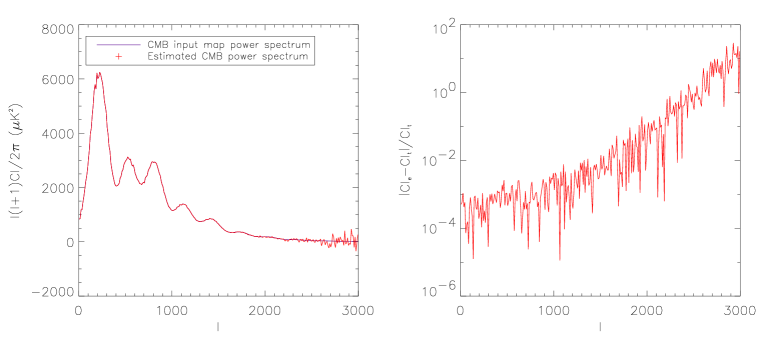
Figure 1: Left: Estimated CMB power spectrum and CMB power spectrum of the input map. Right: Relative errors made on the CMB power spectrum estimation.

6 Conclusion

We have presented our blind spectral matching method for all-sky multi-detector CMB observations. The main objective is to measure the power spectra of all the components, including the CMB, and their contribution levels at each observation frequency. The method exploits in particular the cross-power spectra of observation maps, giving an unbiased estimate of component power spectra. The method has been applied on full-sky Planck simulations containing five components and white noise. The power spectrum of the CMB is accurately estimated up to $l\simeq 2000$ in bins of size $\Delta l=10$.

Acknowledgments. The author would like to thank the Planck collaboration and in particular M.A.J. Ashdown, V. Stolyarov and R. Kneissl for the full sky simulated maps, and also J. Bartlett for a critical reading of the manuscript. The HEALPix package (see http://www.eso.org/ science/healpix/) was used for the spherical harmonics decomposition of the input maps.

References

- [1] F.R. Bouchet and R. Gispert, New Astronomy, vol. 4, pp. 443-479, Nov. 1999.
- [2] A. Benoît et al., Astronomy and Astrophysics, vol. 399, pp. 19-23, Mar. 2003
- [3] J.F. Cardoso et al., 2002, EUSIPCO proceedings, Vol. 1, pp 561-564.
- [4] J. Delabrouille et al., astro-ph/0211504, submitted to MNRAS.
- [5] M.P. Hobson et al., MNRAS, vol. 300, pp. 1-29, Oct. 1998.
- [6] G. Patanchon et al., 2003, PSIP03 proceedings, pp. 17-20.
- [7] S. Prunet et al., Astronomy and Astrophysics, vol. 373, pp. 13-16, Jul. 2001.
- [8] V. Stolyarov et al., MNRAS, vol. 336, pp. 97-111, Oct. 2002.
- [9] M. Tegmark and G. Efstathiou, MNRAS, vol. 281, pp. 1297-1314, Aug. 1996.
- [10] C.L. Kuo et al., American Astronomical Society Meeting, vol 201, Dec. 2002.
- [11] P. De Bernardis et al., Nature, vol. 404, pp. 955-959, Apr. 2000.
- [12] S. Hanany et al., The Astrophysical Journal, vol. 545, pp. 5-9, Dec. 2000.
- [13] B. Mason et al., American Astronomical Society Meeting, vol. 199, Dec. 2001.
- [14] N.W. Halverson et al., The Astrophysical Journal, vol. 568, pp. 38-45, Mar. 2002.
- [15] K. Grainge et al., MNRAS, vol. 341, pp. 23-28, Jun. 2003
- [16] G. Hinshaw et al., astro-ph/0302217