Abstract

The discrete-dipole approximation (DDA) is a powerful method for calculating absorption and scattering by targets that have sizes smaller than or comparable to the wavelength of the incident radiation. We present a new prescription – the Surface-Corrected Lattice Dispersion Relation (SCLDR) – for assigning the dipole polarizabilities that takes into account both target geometry and finite wavelength. We test the SCLDR in DDA calculations using spherical and ellipsoidal targets and show that for a fixed number of dipoles, the SCLDR prescription results in increased accuracy in the calculated cross sections for absorption and scattering. We discuss extension of the SCLDR prescription to irregular targets.

OCIS codes: 000.4430, 240.0240, 260.2110, 290.5850.

1 Introduction

The discrete-dipole approximation (DDA) is a numerical technique for calculating scattering and absorption of electromagnetic radiation by targets with sizes smaller than or comparable to the incident wavelength. The method consists of approximating the target by an array of polarizable points (dipoles), assigning polarizabilities at these locations based on the physical properties of the target, and solving self-consistently for the polarization at each location in the presence of an incident radiation field. This procedure can yield arbitrarily accurate results as the number of dipoles used to approximate the target is increased. However, computational considerations limit the number of dipoles that can be used. Hence, methods for increasing the accuracy for a fixed number of dipoles are desirable.

A key factor in determining the level of accuracy that can be reached for a given number of dipoles is the prescription for assigning dipole polarizabilities. In this work, we present a new polarizability prescription that takes into account both target geometry and the finite wavelength of incident radiation. We test this technique in calculations of absorption and scattering by spherical and ellipsoidal targets and show that for a fixed number of dipoles, it generally provides increased accuracy over previous methods. In Section 2 we discuss previous polarizability prescriptions and develop the new method. In Section 3 we present calculations testing the new prescription, and in Section 4 we discuss our results.

2 Polarizability Prescriptions

A fundamental requirement of the DDA is that the inter-dipole separation $d$ be small compared to the wavelength of incident radiation, $kd\leq 1$, where $k\equiv\omega/c$ is the wavenumber in vacuo. Here we will assume the dipoles to be located on a cubic lattice with lattice constant $d$, as this facilitates use of fast-Fourier transform (FFT) techniques .${}^{\hbox{\immediate{\bf{?}}}}$

The first implementations of the DDA ${}^{\hbox{\immediate{\bf{?}}}}$ used the so-called Clausius-Mossotti relation (CMR) to determine the dipole polarizabilities. In this procedure, the polarizability $\alpha$ is given as a function of the (complex) refractive index $m$ as

$$\alpha_{\rm CMR}={{3d^{3}}\over{4\pi}}\left({{m^{2}-1}\over{m^{2}+2}}\right),$$ (1)

This approach is valid in the infinite wavelength limit of the DDA, $kd\rightarrow 0$.

Draine ${}^{\hbox{\immediate{\bf{?}}}}$ showed that for finite wavelengths, the optical theorem requires that the polarizabilities include a “radiative-reaction” correction of the form

$$\alpha={{\alpha^{(nr)}}\over{1-(2/3)i(\alpha^{(nr)}/d^{3})(kd)^{3}}},$$ (2)

where $\alpha^{(nr)}$ is the “non-radiative” polarizability, that is, before any radiative-reaction correction is applied. Draine ${}^{\hbox{\immediate{?}}}$ used $\alpha_{\rm CMR}$ as the non-radiative polarizability.

Based on analysis of an integral formulation of the scattering problem, Goedecke & O’Brien ${}^{\hbox{\immediate{\bf{?}}}}$ and Hage & Greenberg ${}^{\hbox{\immediate{\bf{?}}}}$ suggested further corrections to the CMR polarizability of order $(kd)^{2}$. Draine & Goodman ${}^{\hbox{\immediate{\bf{?}}}}$ studied electromagnetic wave propagation on an infinite lattice; they required that the lattice reproduce the dispersion relation of a continuum medium. In this “Lattice Dispersion Relation” (LDR) approach, the radiative-reaction correction emerges naturally, and the polarizability is given [to order $(kd)^{3}$] by

$$\alpha_{\rm LDR}={{\alpha^{(0)}}\over{1+(\alpha^{(0)}/d^{3})[(b_{1}+m^{2}b_{2}+m^{2}b_{3}S)(kd)^{2}-(2/3)i(kd)^{3}]}},$$ (3)

where $\alpha^{(0)}=\alpha_{\rm CMR}$ is the polarizability in the limit $kd\rightarrow 0$, $b_{1}=-1.8915316$, $b_{2}=0.1648469$ and $b_{3}=-1.7700004$, and $S$ is a function of the propagation direction and polarization of the incident wave. $S$ is given as

$$S=\sum_{j}(a_{j}e_{j})^{2},$$ (4)

where $\bf a$ and $\bf e$ are the unit propagation and polarization vectors, respectively. Note that eq. (4) gives $S=0$ for waves propagating along any of the lattice axes. This method correctly accounts to $O[(kd)^{3}]$ for the finite wavelength of incident radiation, and by construction, it accurately reproduces wave propagation in an infinite medium. Its primary limitation is that the accuracy in computing absorption cross-sections of finite targets (for a given number of dipoles) degrades rapidly as the imaginary part of the refractive index $m$ becomes large (e.g., for ${\mathrm{Im}}(m)\geq 2$).

A Geometric Corrections: the Static Case

Recently Rahmani, Chaumet & Bryant ${}^{\hbox{\immediate{\bf{?}}}}$ (RCB) proposed a new method for assigning the polarizabilities that takes into account the effects of target geometry on the local electric field at each dipole site. Consider a continuum target in a static, uniform applied field ${\bf E}^{0}$. At each location $i$ in the target, the macroscopic electric field ${\bf E}_{i}^{m}$ is linearly related to ${\bf E}^{0}$:

$${\bf E}_{i}^{m}={\bf C}_{i}^{-1}{\bf E}^{0}$$ (5)

where ${\bf C}_{i}^{-1}$ is a $3\times 3$ tensor that will depend on location $i$, the global geometry of the target, and its (possibly nonuniform) composition. If we now represent the target by a dipole array, and require that the electric dipole moment ${\bf P}_{i}$ of dipole $i$ be equal to $d^{3}$ times the macroscopic polarization density at location $i$, we obtain

$${\bf P}_{i}=d^{3}\left(\frac{\epsilon_{i}-1}{4\pi}\right){\bf E}_{i}^{m}=d^{3}\left(\frac{\epsilon_{i}-1}{4\pi}\right){\bf C}_{i}^{-1}{\bf E}^{0}$$ (6)

If ${\hbox{\boldsym\char 11\relax}}_{i}$ is the polarizability tensor of dipole $i$, then

$${\bf P}_{i}={\hbox{\boldsym\char 11\relax}}_{i}\left[{\bf E}^{0}-\sum_{j\neq i}{\bf A}_{ij}{\bf P}_{j}\right]$$ (7)

where $-{\bf A}_{ij}{\bf P}_{j}$ is the contribution to the electric field at location $i$ due to dipole ${\bf P}_{j}$ at location $j$ (this defines the 3$\times$3 tensors ${\bf A}_{ij}$). Substituting (6) into (7) we obtain

$${\hbox{\boldsym\char 11\relax}}_{i}=d^{3}\left(\frac{\epsilon_{i}-1}{4\pi}\right){\bf\Lambda}_{i}^{-1}$$ (8)

where the 3$\times$3 tensors

$${\bf\Lambda}_{i}\equiv{\bf C}_{i}-\sum_{j\neq i}{\bf A}_{ij}\left(\frac{\epsilon_{j}-1}{4\pi}\right)d^{3}{\bf C}_{j}^{-1}{\bf C}_{i}$$ (9)

can be evaluated (and easily inverted) if the ${\bf C}_{i}$ are known.

The RCB approach requires that the tensors ${\bf C}$ first be obtained. For certain simple geometries, the ${\bf C}_{i}$ can be obtained analytically. For example, for homogeneous ellipsoids, infinite slabs, or infinite cylinders, the tensors ${\bf C}_{i}$ can be expressed in the form

$${\bf C}_{i}=1+\left(\frac{\epsilon-1}{4\pi}\right){\bf L}$$ (10)

where ${\bf L}$ is a “depolarization tensor”. For example, $L=1/3$ for a homogeneous sphere.

In the present work, we combine the LDR and RCB approaches in order to obtain a polarizability prescription that accounts both for finite wavelength and for local field corrections arising from target geometry. We adopt ${\hbox{\boldsym\char 11\relax}}_{\rm RCB}$ as the polarizability $\alpha^{(0)}$ in the limit $kd\rightarrow 0$, and apply corrections up to $O[(kd)^{3}]$ based on the LDR. A further analysis of the electromagnetic dispersion relation of a non-cubic lattice ${}^{\hbox{\immediate{\bf{?}}}}$ called into question the value of the constant $b_{3}$ in eq. (3) used by Draine & Goodman ,${}^{\hbox{\immediate{?}}}$ and found it instead to be undetermined by available constraints. Thus we include an adjustable factor $f$ whose value is chosen to optimize the behavior of the new method as discussed in the next section. The “Surface-Corrected Lattice Dispersion Relation” (SCLDR) polarizability is given by

$${\bf{\hbox{\boldsym\char 11\relax}}}_{\rm SCLDR}={\bf{\hbox{\boldsym\char 11\relax}}}_{\rm RCB}\{1+({\bf{\hbox{\boldsym\char 11\relax}}}_{\rm RCB}/d^{3})[(b_{1}+{\bf m}^{2}b_{2}+{\bf m}^{2}b_{3}fS)(kd)^{2}-(2/3)i(kd)^{3}]\}^{-1},$$ (11)

where

$$f=\exp[-0.5{\rm Im}(m)^{2}].$$ (12)

In the next section, we test this new prescription in calculations of absorption and scattering by spherical and ellipsoidal targets.

3 Sphere and Ellipsoid Calculations

For a continuum target of volume $V$, the effective radius $a_{\rm eff}\equiv(3V/4\pi)^{1/3}$, the radius of a sphere of equal volume. The target is approximated by an array of $N$ dipoles located on a cubic lattice, with the dipole locations selected by some criterion designed to approximate the shape of the original target. The inter-dipole spacing is then set to $d=(V/N)^{1/3}$.

For a given orientation of the dipole array relative to the incident wave, we calculate the cross sections $C_{\rm sca}$ and $C_{\rm abs}$ for scattering and absorption, and the dimensionless efficiency factors $Q_{\rm sca}\equiv C_{\rm sca}/\pi a_{\rm eff}^{2}$, $Q_{\rm abs}\equiv C_{\rm abs}/\pi a_{\rm eff}^{2}$.

To test the performance of the SCLDR polarizability prescription against previous results, we performed a series of calculations using the DDA code DDSCAT ,${}^{\hbox{\immediate{\bf{?}}}}$ modified to permit use of the SCLDR polarizabilities. We computed $Q_{\rm sca}$ and $Q_{\rm abs}$ for spherical targets with a range of refractive indexes and for a range of scattering parameters $x=2\pi a_{\rm eff}/\lambda=ka_{\rm eff}$, using three different approaches for assigning the dipole polarizabilities: LDR, RCB and SCLDR. Spherical targets were employed because the exact optical properties can be readily calculated using Mie theory. We also performed a similar but more limited set of calculations for ellipsoidal targets.

We tested the LDR, RCB and SCLDR prescriptions for a number of different refractive indexes in the region of the complex plane with ${\rm Re}(m)\leq 5$ and ${\rm Im}(m)\leq 4$. We determined that for refractive indexes with these ranges of real and imaginary parts, it was desirable for the SCLDR correction factor $f$ to tend toward unity for ${\rm Im}(m)<1$ and to tend toward zero for ${\rm Im}(m)>2$. We chose the functional form of eq. (12) in order to reproduce this asymptotic behavior.

Figures 1 and 2 show the results of calculations for spheres with refractive indices $m=1.33+0.01i$ and $m=5+4i$, each approximated by an array of $N=7664$ dipoles. Because the dipole array is not rotationally symmetric, $Q_{\rm sca}$ and $Q_{\rm abs}$ calculated with the DDA depend in general on the target orientation; we perform calculations for 12 orientations, and we show the average and range of the results. We calculate the fractional errors in $Q_{\rm sca}$ and $Q_{\rm abs}$ by comparison with exact results obtained using Mie theory:

$${\rm frac.err}\equiv\frac{Q({\rm DDA})-Q({\rm Mie})}{Q({\rm Mie})}~{}~{}~{}.$$ (13)

In previous work${}^{\hbox{\immediate{\bf{?}}}}$ it was recommended that the DDA be used only when $|m|kd\leq 1$, or a more stringent condition $|m|kd<0.5$ if the DDA is to be used to calculate the differential scattering cross section. In the present work we find that when the SCLDR polarizabilities are used, the fractional errors in $Q_{\rm sca}$ and $Q_{\rm abs}$ are relatively insensitive to $x$ provided $|m|kd\leq 0.8$, which we adopt as an operational validity criterion. Figures 1 and 2 show results for values of $x$ satisfying $|m|kd\leq 0.8$.

From Figure 1, it is clear that the LDR and SCLDR prescriptions provide approximately equal levels of accuracy in the $|m|\approx 1$ regime, while the RCB prescription does not perform as well. Figure 2 shows that at the other extreme of ${\rm Re}(m)\gg 1$ and ${\rm Im}(m)\gg 1$, the LDR approach results in large errors, especially in the calculated absorption cross sections, while the RCB and SCLDR prescriptions perform approximately equally well.

In Figures 3 and 4, we show the convergence behavior of the different polarizability prescriptions as the number of dipoles $N$ is increased for spherical targets with selected refractive indices; the refractive indices have been chosen to sample the region of the complex plane discussed in the previous paragraphs. The SCLDR method performs comparably to or better than the RCB and LDR prescriptions throughout this region of the complex refractive index plane. This illustrates the advantage of the SCLDR approach over these previous techniques: it performs well not just for a small range of refractive indexes, but for the entire range we have sampled.

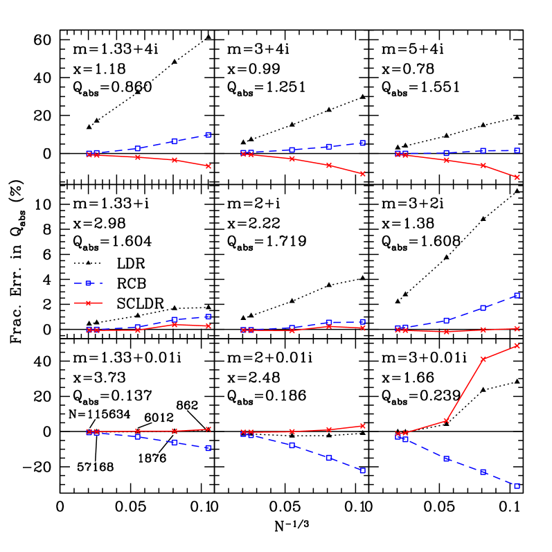
Fig. 5: Same as Fig. 3, but for ellipsoids with approximately 1:2:3 axial ratios. Fractional errors have been estimated based on comparison with an extrapolation of the convergence behavior of the three polarizability prescriptions, as described in Section 3. Again the SCLDR prescription appears comparable or superior to the LDR and RCB prescriptions for calculating $Q_{\rm abs}$ throughout the region of the complex $m$-plane sampled, though the RCB prescription is slightly preferred for the cases of $m=3+4i$ and $m=5+4i$.

Figures 5 and 6 extend the result shown in Figures 3 and 4 to targets of a more general shape, specifically ellipsoids with approximately 1:2:3 axial ratios. For these targets, we have estimated the true values of $Q_{\rm sca}$ and $Q_{\rm abs}$ by assuming these to be linear functions of $N^{-1/3}$, extrapolating to $N^{-1/3}\rightarrow 0$ for each polarizability prescription, and taking the average of the results from the different prescriptions. The close similarity of the results of these calculations to those shown in Figures 3 and 4 demonstrates that the SCLDR prescription provides the same benefits in calculations for ellipsoidal targets as for spheres, although we note that for ellipsoids with values of $m$ with large imaginary parts [typically ${\rm Im}(m)>1$], the RCB prescription can provide improved accuracy in calculations of $Q_{\rm sca}$.

For an isotropic material with refractive index $m$, the Clausius-Mossotti polarizability $\alpha_{\rm CMR}$ has triply-degenerate eigenvalues $\alpha_{\rm CMR}=(m^{2}-1)d^{3}/4\pi$. For the case of a 1:2:3 ellipsoid with refractive index $m=5+4i$, we have calculated the eigenvalues $\alpha$ of ${\hbox{\boldsym\char 11\relax}}_{\rm SCLDR}$ for $|m|kd\rightarrow 0$ (for which case ${\hbox{\boldsym\char 11\relax}}_{\rm SCLDR}\rightarrow{\hbox{\boldsym\char 11\relax}}_{\rm RCB}$) at each occupied lattice site. Figure 7 (left panel) shows the distribution of the fractional difference of the eigenvalues $\alpha$ from $\alpha_{\rm CMR}$. The deviations tend to be appreciable (fractional difference exceeding $\sim$20%) only near the surface. The left panel shows that the deviations exceed 20% for 47% of the lattice sites for $N=90$, but only 9% of the lattice sites when $N=43416$. For this example the fraction of the eigenvalues deviating by $>$20% is $\sim 0.30(N/1000)^{-1/3}$ for $N\geq 500$, approximately equal to the fraction of the dipoles located within a surface layer of thickness $\sim 0.6d$.

The right panel in Figure 7 shows the eigenvalue deviations as a function of distance from the surface of the ellipsoid: the eigenvalues deviating from $\alpha_{\rm CMR}$ by more than $\sim 20\%$ are, as expected, exclusively associated with dipoles located within a distance $d$ of the surface.

4 Conclusion

We introduce a new DDA polarizability prescription – the Surface-Corrected Lattice Dispersion Relation (SCLDR). This technique builds on previous work, principally by Draine & Goodman ${}^{\hbox{\immediate{?}}}$ and Rahmani, Chaumet & Bryant ,${}^{\hbox{\immediate{?}}}$ to account properly for both finite wavelength and target geometry. We have tested the new polarizability prescription in calculations of absorption and scattering by spherical and ellipsoidal targets. These tests show that the SCLDR performs generally better than previous prescriptions which took account either of finite wavelength or of target geometry but not both. The SCLDR technique is most easily applicable to target shapes for which there exists an analytical solution to the electrostatic applied field problem, but it can be applied to any dielectric target (homogeneous or inhomogeneous, isotropic or anisotropic) provided that the electrostatic problem can at least be solved numerically to obtain the tensors ${\bf C}_{i}$ (see eq. 5). In such cases, it generally provides a significant increase in accuracy over previous methods, especially for highly absorptive materials.

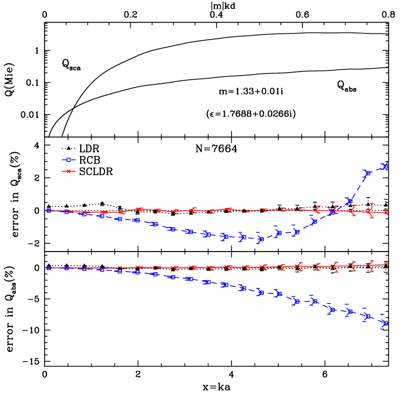
Fig. 1: Comparison of scattering and absorption efficiency factors $Q_{\rm sca}$ and $Q_{\rm abs}$ computed for a pseudo-sphere of $N=7664$ dipoles and refractive index $m=1.33+0.01i$, averaged over 12 orientations, and using three different polarizability prescriptions: Lattice Dispersion Relation (LDR); Rahmani et al. ${}^{\hbox{\immediate{?}}}$ (RCB); and Surface-Corrected Lattice Dispersion Relation (SCLDR). The horizontal axis shows (top) $|m|kd$ (the phase shift in radians within one lattice spacing) and (bottom) the scattering parameter $x=ka$. Error bars indicate the ranges of $Q$ values obtained for the individual orientations. The top panel shows the results of Mie theory calculations; the lower panels show the fractional error in $Q_{\rm sca}$ and $Q_{\rm abs}$, respectively. The SCLDR and LDR prescriptions are clearly preferred over RCB for this case.

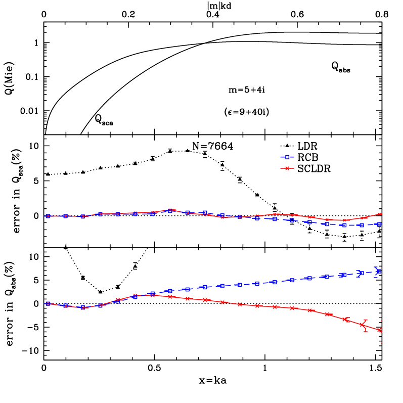
Fig. 2: Same as Fig. 1, but for refractive index $m=5+4i$. The SCLDR and RCB prescriptions are clearly preferred over the LDR for this case, with SCLDR being somewhat superior to RCB.

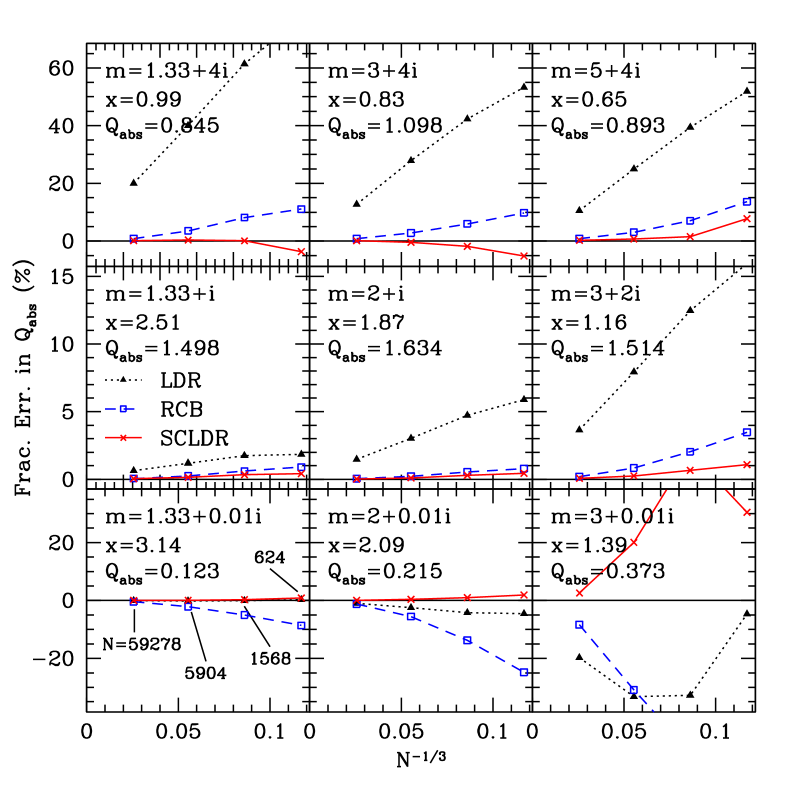
Fig. 3: Fractional error in $Q_{\rm abs}$ averaged over 12 orientations for spheres with different refractive indexes, as a function of $N^{-1/3}$, where $N$ is the number of dipoles, in the range 624–59278. Calculations are shown for the LDR, RCB, and SCLDR polarizability prescriptions; the symbolic scheme is the same as in Fig. 1. Refractive indexes $m$, scattering parameters $x=ka$, and exact values of $Q_{\rm abs}$ computed from Mie theory are shown in the left portion of each panel. The scattering parameters are chosen so that $|m|kd\approx 0.8$ (the approximate limit of applicability of the DDA) for the smallest number ($N=624$) of dipoles. The convergence with increasing $N$ is quite smooth in all regions of the complex $m$-plane, with the exception of $m=3+0.01i$. In almost every case shown, fractional errors $<2$% (and often significantly lower) can be achieved for $N\approx 6000$ dipoles. We find that for calculating $Q_{\rm abs}$, the SCLDR is comparable or superior in accuracy to the LDR and RCB prescriptions throughout the region of $m$-space shown.

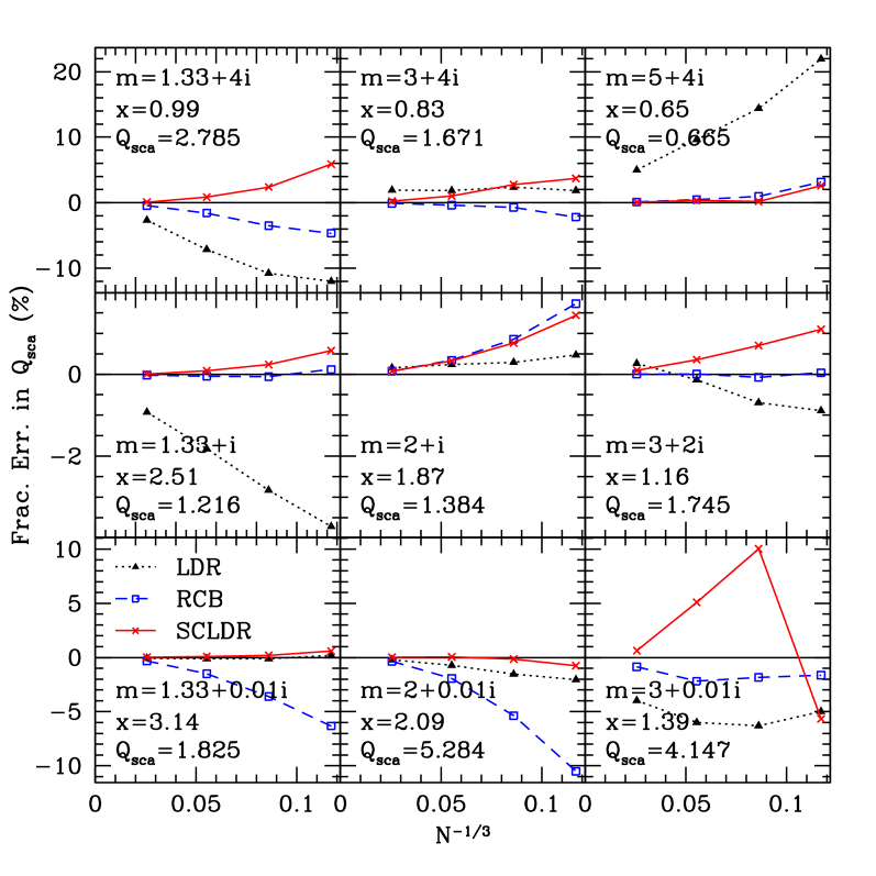
Fig. 4: Same as Fig. 3, except that fractional errors in $Q_{\rm sca}$ are plotted. Again, the SCLDR prescription is comparable or superior to the LDR prescription for all values of $m$ shown. While the SCLDR prescription is still comparable or superior to the RCB prescription for $m$ values with small imaginary parts, the RCB prescription provides better accuracy in calculating $Q_{\rm sca}$ for $m$ values with large imaginary parts.

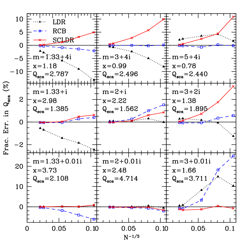
Fig. 6: Same as Fig. 5, except that fractional errors in $Q_{\rm sca}$ are plotted. As in Fig. 3, SCLDR is comparable to or superior to LDR for all values of $m$, and to RCB for values of $m$ with small imaginary parts, while RCB is somewhat superior to SCLDR for values of $m$ with large imaginary parts.

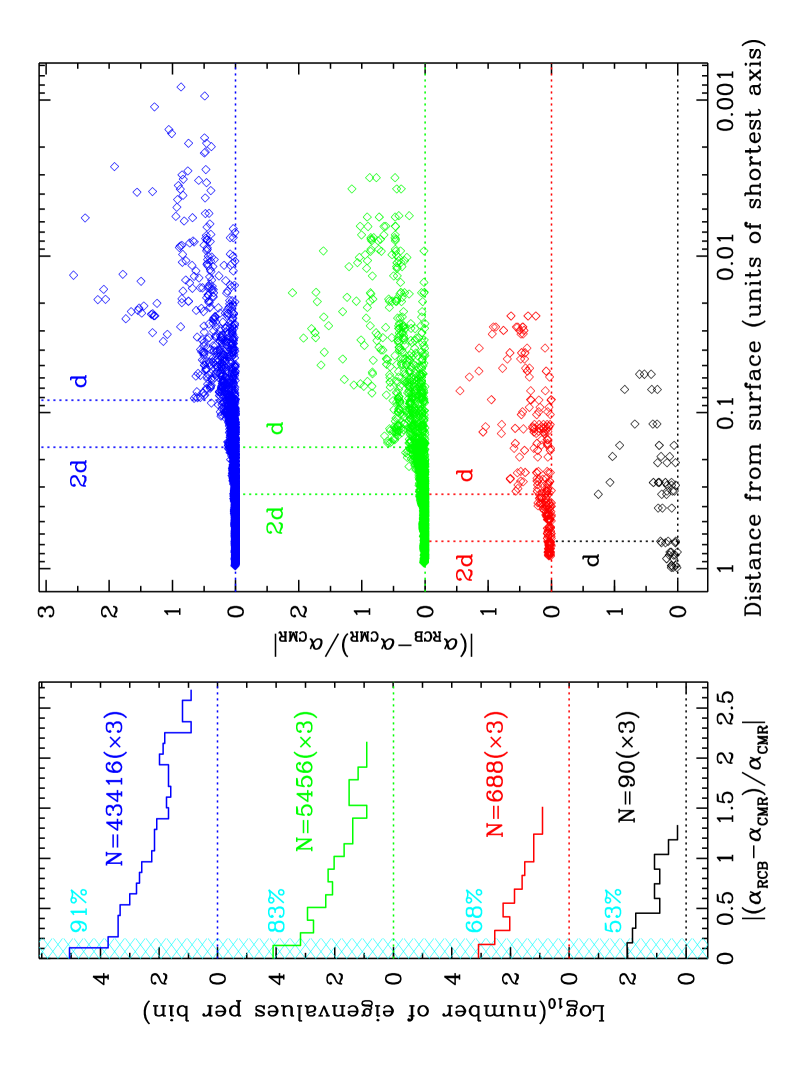
Fig. 7: Comparison of RCB and CMR polarizabilities. The left panel shows the distribution of polarizability eigenvalues for discrete dipole approximations to a 1:2:3 ellipsoid with $m=5+4i$ using $N=90$, 688, 5456, and 43416 dipoles. The shaded region corresponds to a fractional difference of 20% or less; the fraction of the eigenvalues within this region varies from 53% for $N=90$ ($3d\times 6d\times 9d$ axes) to 91% for $N=43416$ ($24d\times 48d\times 72d$ axes). The right panel shows the fractional difference between RCB and CMR polarizabilities versus the distance (in units of the shortest axis) from the ideal ellipsoidal surface used to define the target (all dipole locations are interior to this surface). As expected, the RCB polarizability reduces to the CMR polarizability for dipoles lying more than $\sim$2$d$ from the surface.

References

- [1] J. J. Goodman, B. T. Draine, and P. J. Flatau, “Application of fast-Fourier transform techniques to the discrete dipole approximation,” Opt. Lett. 16, 1198–1200 (1990).
- [2] E. M. Purcell and C. R. Pennypacker, “Scattering and absorption of light by nonspherical dielectric grains,” Astrophys. J. 186, 705–714 (1973).
- [3] B. T. Draine, “The discrete-dipole approximation and its application to interstellar graphite grains,” Astrophys. J. 333, 848–872 (1988).
- [4] G. H. Goedecke and S. G. O’Brien, “Scattering by irregular inhomogeneous particles via the digitized Green’s function algorithm,” Appl. Opt. 27, 2431–2438 (1988).
- [5] J. I. Hage and J. M. Greenberg, “A model for the optical properties of porous grains,” Astrophys. J. 361, 251–259 (1990).
- [6] B. T. Draine and J. Goodman, “Beyond Clausius-Mossotti: wave propagation on a polarizable point lattice and the discrete dipole approximation,” Astrophys. J. 405, 685–697 (1993).
- [7] A. Rahmani, P. C. Chaumet, and G. W. Bryant, “Coupled dipole method with an exact long-wavelength limit and improved accuracy at finite frequencies,” Opt. Lett. 27, 2118–2120 (2002).
- [8] D. Gutkowicz-Krusin and B. T. Draine, in preparation
- [9] B. T. Draine and P. J. Flatau, “User Guide for the Discrete Dipole Approximation Code DDSCAT (Version 5a10),” http://xxx.arXiv.org/abs/astro-ph/0008151v3, 1–42 (2000).
- [10] B. T. Draine and P. J. Flatau, “The discrete dipole approximation for scattering calculations”, J. Opt. Soc. Am. A, 11, 1491–1499 (1994).