Photometric Properties of Lyman-break Galaxies at $z=3$ in Cosmological SPH Simulations

Abstract

We study the photometric properties of Lyman-break galaxies (LBGs) formed by redshift $z=3$ in a set of large cosmological smoothed-particle hydrodynamics (SPH) simulations of the $\Lambda$ cold dark matter ($\Lambda$CDM) model. Our numerical simulations include radiative cooling and heating with a uniform UV background, star formation, supernova feedback, and a phenomenological model for galactic winds. Analysing a series of simulations of varying box size and particle number allows us to isolate the impact of numerical resolution on our results. We compute spectra of simulated galaxies using a population synthesis model, and derive colours and luminosity functions of galaxies at $z=3$ after applying local dust extinction and absorption by the intergalactic medium (IGM). We find that the simulated galaxies have $U_{n}-G$ and $G-R$ colours consistent with observations, provided that intervening absorption by the IGM is applied. The observed properties of LBGs, including their number density, colours, and luminosity functions, can be explained if LBGs are identified with the most massive galaxies at $z=3$, having typical stellar mass of $M_{\star}\sim 10^{10}\,h^{-1}{\rm M_{\odot}}$, a conclusion broadly consistent with earlier studies based on hydrodynamic simulations of the $\Lambda$CDM model. We also find that most simulated LBGs were continuously forming stars at a high rate for more than one Gyr up until $z=3$, but with numerous starbursts lying on top of the continuous component. Interestingly, our simulations suggest that more than 50% of the total stellar mass and star formation rate in the Universe are accounted for by galaxies that are not detected in the current generation of LBG surveys.

1 Introduction

Based on surveys made with modern large telescopes, the number of observed Lyman-break galaxies (LBGs; e.g. Steidel, Pettini, & Hamilton, 1995) has reached about $\sim 1000$ (Steidel et al., 2003) by now, providing a unique window for studying early galaxy formation. In these observations, a large sample of LBG-candidates is first selected as “drop-outs” in certain sets of colour-colour planes (e.g. $U_{n}-G$ vs. $G-R$), and then later spectroscopic follow-up observations are performed to obtain the redshifts of the identified candidates. Most surveys to date have been carried out at optical wavelengths, corresponding to the rest-frame far ultra-violet (UV) at redshift $z=3$. The LBGs found in this way show strong clustering (Adelberger et al., 1998; Giavalisco et al., 1998; Steidel et al., 1998), which has generally been interpreted as indirect evidence that LBGs reside in massive dark matter halos. Several studies of LBGs based on semi-analytic models for galaxy formation agree with the massive dark matter halo hypothesis (e.g. Mo & Fukugita, 1996; Baugh et al., 1998; Kauffmann et al., 1999; Mo, Mao, & White, 1999), but a numerical study by Jing & Suto (1998) using collisionless N-body simulations expressed some concerns whether the clustering of dark matter halos of $<10^{12}\,h^{-1}{\rm M_{\odot}}$ can explain the observed clustering strength of LBGs. However, a later investigation by Katz, Hernquist & Weinberg (1999) argued that the CDM models have no difficulty in explaining the strong observed clustering of LBGs, although the substantial box size effects in their analysis introduced some uncertainty.

More recently, LBGs have also been studied in the near infrared (IR) (Sawicki & Yee, 1998; Papovich, Dickinson, & Ferguson, 2001; Pettini et al., 2001; Shapley et al., 2001; Rudnick et al., 2001). Near IR observations are less affected by dust obscuration and directly probe the rest-frame optical properties of LBGs at $z=3$. Therefore, they allow a more reliable derivation of the stellar masses of LBGs. Based on these observations, it has been suggested that the value of the extinction lies in the range $E(B-V)\approx 0.0-0.3$ with a median value of 0.15, and that a significant old stellar population exists in LBGs at $z=3$, with a stellar mass of $\approx 10^{10}\rm M_{\odot}$ (Papovich et al., 2001; Shapley et al., 2001). The existence of such a stellar component would again suggest that LBGs are embedded in massive dark matter halos which have continuously formed stars over an extended period of roughly one Gyr up to $z=3$. These systems would then most likely evolve into elliptical galaxies at the present day, or into the spheroidal components of massive spiral galaxies.

However, in a competing model, LBGs have been suggested to be merger-induced starbursting systems associated with low-mass halos (Lowenthal et al., 1997; Sawicki & Yee, 1998; Somerville, Primack, & Faber, 2001), and in some cases merger-induced starbursts are given a crucial role even when LBGs are the most massive galaxies at their time (Somerville et al., 2001). Given that the merger rate is expected to be quite high at $z\simeq 3$, these scenarios provide an interesting alternative to the more conventional picture which associates LBGs with the most massive systems.

Self-consistent hydrodynamic simulations are an ideal tool for trying to distinguish between these different scenarios for the nature of LBGs. Davé et al. (1999) and Weinberg, Hernquist & Katz (2002) were the first to employ smoothed particle hydrodynamics (SPH) simulations to this end. However, their box size of $11.1\,h^{-1}{\rm\,Mpc}$ represented an important limitation, because the space-density of LBGs is so low that only a few of them can be found in a volume of this size, as we will discuss further in Section 4. Therefore, simulations with a larger box size are desirable to obtain larger samples of simulated LBGs. Nagamine (2002) used an Eulerian hydrodynamic simulation with a box size of ${L_{\rm box}}=25\,h^{-1}{\rm\,Mpc}$, tracing the merger history of galaxies from $z=5$ to $z=0$. The results of these earlier numerical studies were consistent with each other, and agreed reasonably well with the observations, within the uncertainties. In particular, the median stellar masses of LBGs were predicted to be $\sim 10^{10}\,h^{-1}{\rm M_{\odot}}$, and the simulated galaxies were experiencing significant star formation rates ($>30\,\rm M_{\odot}/{\rm yr}$) for extended periods of time ($\geq 1$ Gyr).

Run	Box Size	${N_{\rm p}}$	$m_{\rm DM}$	$m_{\rm gas}$	$\epsilon$	$z_{\rm end}$	wind
O3	10.00	$2\times 144^{3}$	$2.42\times 10^{7}$	$3.72\times 10^{6}$	2.78	2.75	none
P3	10.00	$2\times 144^{3}$	$2.42\times 10^{7}$	$3.72\times 10^{6}$	2.78	2.75	weak
Q3	10.00	$2\times 144^{3}$	$2.42\times 10^{7}$	$3.72\times 10^{6}$	2.78	2.75	strong
Q4	10.00	$2\times 216^{3}$	$7.16\times 10^{6}$	$1.10\times 10^{6}$	1.85	2.75	strong
Q5	10.00	$2\times 324^{3}$	$2.12\times 10^{6}$	$3.26\times 10^{5}$	1.23	2.75	strong
D4	33.75	$2\times 216^{3}$	$2.75\times 10^{8}$	$4.24\times 10^{7}$	6.25	1.00	strong
D5	33.75	$2\times 324^{3}$	$8.15\times 10^{7}$	$1.26\times 10^{7}$	4.17	1.00	strong
G5	100.0	$2\times 324^{3}$	$2.12\times 10^{9}$	$3.26\times 10^{8}$	8.00	0.00	strong
G6	100.0	$2\times 486^{3}$	$6.29\times 10^{8}$	$9.67\times 10^{7}$	5.00	0.00	strong

Table 1: Simulations employed in this study. The box size is given in units of $h^{-1}{\rm\,Mpc}$, ${N_{\rm p}}$ is the particle number of dark matter and gas (hence $\times\,2$), $m_{\rm DM}$ and $m_{\rm gas}$ are the masses of dark matter and gas particles in units of $\,h^{-1}{\rm M_{\odot}}$, respectively, $\epsilon$ is the comoving gravitational softening length in units of $h^{-1}{\rm\,kpc}$, and $z_{\rm end}$ is the ending redshift of the simulation. The value of $\epsilon$ is a measure of spatial resolution. From the top to the bottom row, we collectively call the first 5 runs (O3 to Q5) ‘Q-series’, D4 & D5 are called ‘D-series’, and G5 & G6 are called ‘G-series’.

In this paper, we improve on the earlier numerical studies of LBGs by using a new set of high-resolution numerical simulations. These simulations are based on a novel model for the physics of star formation and feedback, and they use a more accurate implementation of SPH. For the first time, we also systematically study the effects of resolution and box size in the context of simulated LBG galaxies. The treatment of star formation and feedback we use is based on a sub-resolution multi-phase description of the dense, star-forming interstellar medium (ISM), and a phenomenological model for strong feedback by galactic winds, as recently proposed by Springel & Hernquist (2003a). This model has been shown to provide converged star formation rates for well-resolved galaxies, with a cosmic star formation history consistent with recent observations (Springel & Hernquist, 2003b; Hernquist & Springel, 2003). The inclusion of winds was motivated by the realisation that galactic outflows at high redshift (Pettini et al., 2002) likely play a key role in distributing metals into the intergalactic medium (e.g. Aguirre et al., 2001a, b), as well as being important for the regulation of star formation activity. In fact, winds may also alter the distribution of neutral gas around galaxies (Adelberger et al., 2003), although the details of how this process may happen remain unclear (e.g. Croft et al., 2002; Kollmeier et al., 2003; Bruscoli et al., 2003). In passing, we note that both Desjacques et al. (2003) and Maselli et al. (2003) have found that the Lyman-$\alpha$ transmissivity close to LBGs, as measured by Adelberger et al. (2003), is better reproduced if LBGs are identified as dwarf starbursting galaxies as proposed in Somerville et al. (2001) and Weatherley & Warren (2003). We will discuss the work of Weatherley & Warren (2003) in Section 8. Together with the increase in numerical resolution provided by our simulations, it is of interest to see how our refined physical modelling modifies the predictions for LBG properties within the $\Lambda$CDM scenario.

This paper is organised as follows. In Section 2, we briefly introduce the numerical parameters of our simulation set. In Section 3, we then describe our method for computing spectra of simulated galaxies both in the rest-frame and the observed frame. In Sections 4 and 5, we show the colour-colour diagrams and colour-magnitude diagrams of simulated galaxies, and we discuss the number density of colour-selected LBGs, as well as the stellar masses of LBGs at $z=3$. We then investigate the rest-frame $V$-band luminosity function and observed $R$-band luminosity function in Section 6, followed by an analysis of the star formation histories of LBGs in Section 7. Finally, we summarise and discuss the implications of our work in Section 8.

2 Simulations

We analyse a large set of cosmological SPH simulations with varying box size, mass resolution and feedback strength, as summarised in Table 1. Our box size ranges from 10 to $100\,h^{-1}{\rm\,Mpc}$ on a side, with particle numbers between $2\times 144^{3}$ and $2\times 486^{3}$, giving gaseous mass resolutions in the range $3.3\times 10^{5}$ to $3.3\times 10^{8}\,h^{-1}{\rm M_{\odot}}$. These simulations are partly taken from a study of the cosmic star formation history by Springel & Hernquist (2003b), supplemented by additional runs with weaker or no galactic winds. A similar set of simulations was used by Nagamine, Springel, & Hernquist (2004a, b) to study the properties of damped Lyman-$\alpha$ absorbers, but here we analyse the ‘G6’-run which has higher resolution than the ‘G4’-run used in the previous studies. The simulations with the same box size are run with the same initial condition.

There are three main novel features to our simulations. First, we use the new “conservative entropy” formulation of SPH (Springel & Hernquist, 2002) which explicitly conserves entropy (in regions without shocks), as well as momentum and energy, even when one allows for fully adaptive smoothing lengths (see e.g. Hernquist, 1993). This formulation moderates the overcooling problem present in earlier formulations of SPH (see also Yoshida et al., 2002; Pearce et al., 1999; Croft et al., 2001).

Second, highly over-dense gas particles are treated with an effective sub-resolution multiphase ISM model, as described by Springel & Hernquist (2003a). In this model, each gas particle represents a statistical mixture of cold clouds and a hot ambient phase. Cold clouds can grow by radiative cooling out of the hot medium, and form the reservoir of neutral gas for star formation. Once star formation takes place, supernova explosions deposit energy into the hot gas, heating the gas and evaporating the cold clouds, transferring cold gas back into the hot phase. This feedback establishes a self-regulated cycle of star formation.

Third, a phenomenological model for galactic winds is implemented. In this model, gas particles are stochastically driven out of the dense star-forming region by assigning an extra momentum in random directions, with a rate and magnitude chosen to reproduce mass-loads and wind speeds similar to those observed. (See Springel & Hernquist (2003a) for a detailed discussion of this method.) Most of our simulations employ a “strong” wind of speed $484\,{\rm km\,s^{-1}}$, but for the O3, P3, & Q3-runs, we also varied the wind strength to examine the effect of feedback from galactic winds. The runs with $10\,h^{-1}{\rm\,Mpc}$ boxes are collectively called the ‘Q-series’, and the resolution is increased from Q3 to Q4, and to Q5. The other series (‘D-’and ‘G-Series’) extend the strong wind results to larger box sizes and hence lower redshift. Our naming convention is such that runs of the same model (box size and included physics) are designated with the same letter, with an additional number specifying the particle resolution.

Our calculations include a uniform UV background radiation field with a modified Haardt & Madau (1996) spectrum, where reionisation takes place at $z\simeq 6$ (see Davé et al., 1999) as suggested by the quasar observations (e.g. Becker et al., 2001) and radiative transfer calculations of the impact of the stellar sources in our simulations on the IGM (e.g. Sokasian et al., 2003). The early reionisation at higher redshift, as suggested by the WMAP satellite, should not affect the results presented in this paper because we are mainly dealing with halos with virial temperatures above $10^{4}$ K and the infalling gas will radiatively cool even if it was photoionised by the reionisation at $z>10$ before falling into the halo (see Springel & Hernquist, 2003b). The radiative cooling and heating rate is computed as described by Katz et al. (1996) assuming that the gas is optically thin and in ionisation equilibrium. The adopted cosmological parameters of all runs are $(\Omega_{\rm m},\Omega_{\Lambda},\Omega_{\rm b},\sigma_{8},h)=(0.3,0.7,0.04,0.9,0.7)$. The simulations were performed on the Athlon-MP cluster at the Center for Parallel Astrophysical Computing (CPAC) at the Harvard-Smithsonian Center for Astrophysics, using a modified version of the parallel GADGET code (Springel, Yoshida & White, 2001).

3 Method

We identify simulated galaxies as isolated groups of stars using a simplified variant of the SUBFIND algorithm proposed by Springel et al. (2001). In detail, we first compute an adaptively smoothed baryonic density field for all star and gas particles, allowing us to robustly identify centres of individual galaxies as isolated density peaks. We find the full extent of these galaxies by processing the gas and star particles in the order of declining density, adding particles one by one to the galaxies. If all of the 32 nearest neighbours of a particle have lower density, this particle is considered to be a new galaxy ‘seed’. Otherwise, the particle is attached to the galaxy that its nearest denser neighbour already belongs to. If the two nearest denser neighbours belong to different galaxies, and one of these galaxies has less than 32 particles, these galaxies are merged. If the two nearest denser neighbours belong to different galaxies and both of these galaxies have more than 32 particles, then the particle is attached to the larger group of the two, leaving the other one intact. Finally, we restrict the set of gas particles processed in this way to those particles which have at least a density of $0.01$ times the threshold density for star formation, i.e. $\rho_{\rm th}=8.6\times 10^{6}h^{2}\rm M_{\odot}{\rm kpc}^{-3}$ (see Springel & Hernquist, 2003a, for details on how this parameter is determined). Note that we are not interested in the gaseous components of galaxies – we only include gas particles because they make the method more robust. Since most galaxies contain very dense star-forming gas, such a method make it particularly easy to select galaxies when the gas is included.

We found that the above method robustly links up star particles that belong to the same isolated galaxy. A simpler FoF algorithm with a small linking length can achieve a largely similar result, but the particular choice for the linking length one needs to make in this method represents a problematic compromise, either leading to artificial merging of galaxies if it is selected too large, or to loss of star particles that went astray from the dense galactic core, if selected too small. Note that, unlike in the detection of dark matter substructures, no gravitational unbinding algorithm is needed to define the groups of stars that make up the galaxies formed in the simulations.

We only consider galaxies with at least 32 particles (star and gas combined) in our subsequent analysis. Each stellar particle contained in them is tagged by the simulation code with its mass, formation time, and metallicity of the gas particle that it formed out of. Based on these three tags, we compute the emission from each stellar particle, and co-add the flux from all particles for a given galaxy to obtain the spectrum of the simulated galaxy. We use the population synthesis model GISSEL99 (Bruzual & Charlot, 1993) that assumes the Salpeter (1995) initial mass function with a mass range of $[0.1,125]\,\rm M_{\odot}$.

Once the intrinsic spectrum is computed, we apply the Calzetti extinction law (Calzetti et al., 2000) with three different values of $E(B-V)=0.0,0.15,0.3$ to investigate the effects of extinction. These values span the range of $E(B-V)$ estimated from observations of LBGs at $z=3$ (Adelberger & Steidel, 2000; Shapley et al., 2001). Rest-frame colours and luminosity functions of the simulated galaxies are then derived using the spectra computed in this manner.

To obtain the spectra in the observed frame, we redshift the spectra and apply absorption by the IGM following the prescription by Madau (1995). Once the redshifted spectra in the observed frame are obtained, we convolve them with various filter functions, including $U_{n},G,R$ (Steidel & Hamilton, 1993) and standard Johnson bands, and compute the magnitudes in both AB and Vega systems. Apparent $U_{n}$, $G$, $R$ magnitudes are computed in the AB system to compare our results with Steidel et al. (2003), while the rest-frame V-band magnitude is computed in the Vega system to compare our results with those of Shapley et al. (2001).

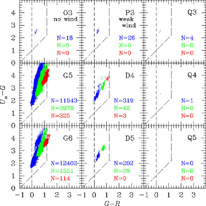
Figure 1: Colour-colour diagrams ($U_{n}-G$ vs. $G-R$) of simulated galaxies at $z=3$ with apparent $R$ magnitudes brighter than $R<25.5$. Three different symbols represent three different values of extinction: $E(B-V)=0.0$ (blue dots), 0.15 (green crosses), and 0.3 (red open squares). The number of simulated galaxies of each type is indicated from top to bottom in each panel, respectively. The dashed lines mark the colour-colour selection criteria used by Steidel et al. (2003) to identify LBG candidates at $z\sim 3$.

4 Colour-colour diagrams

In Figure 1, we show the colour-colour magnitude diagrams of simulated galaxies at $z=3$ in the $U_{n}-G$ vs. $G-R$ plane, for galaxies brighter than $R=25.5$ (the magnitude cut used by Steidel et al., 2003). The three different symbols represent three different values of Calzetti extinction: $E(B-V)=0.0$ (blue dots), 0.15 (green crosses), and 0.3 (red open squares). The long-dashed lines mark the colour-colour selection criteria applied by Steidel et al. (2003) to identify LBG candidates at $z\sim 3$.

It is encouraging to see that in all the panels most of the simulated galaxies actually satisfy the observational colour selection criteria. This suggests that the simulated galaxies have realistic colours compared to the observed LBGs at $z=3$. In runs with larger box size (D- and G-series), the distribution is wider than the one in the ${L_{\rm box}}=10\,h^{-1}{\rm\,Mpc}$ runs (Q-series), and the distribution actually extends beyond the colour selection boundaries of Steidel et al. (2003). The box size of the Q-series (${L_{\rm box}}=10\,h^{-1}{\rm\,Mpc}$) is too small to contain a significant sample of LBGs, and no LBGs with $R<25.5$ can be found in the Q-series for the cases of $E(B-V)=0.15$ and 0.3.

If we had not applied the Madau (1995) absorption to the spectra, the distribution would not have fallen into the colour selection region. This is because the simulated galaxies would then appear too bright in the UV, such that the distribution would fall below $U_{n}-G<1.0$. As the level of extinction by dust is increased from $E(B-V)=0.0$ to 0.3, the measured points move towards the upper right corner of each panel. This behaviour is expected for a standard star-forming galaxy spectrum, as demonstrated in Figure 2 of Steidel et al. (2003). At the same time, the number of galaxies that satisfy the magnitude cut of $R=25.5$ decreases with increasing extinction, because stronger extinction results in a redder galaxy spectrum.

Note that increasing the resolution from Q3 to Q4, and then to Q5, also reduces the number of galaxies brighter than $R=25.5$ slightly. The same is true for D4 and D5 runs. As the resolution is increased, not only are the most massive halos in the simulation better resolved, but also all of their progenitors. The better resolution then allows a more accurate treatment of the wind-feedback in these progenitor generations of galaxies; the net result of this is a decrease in the final luminosity of the brightest galaxies. For the ‘Q5’-run, there are actually no galaxies brighter than $R=25.5$.

This is not the case for the lower resolution, larger box size simulations where the trend appears to reverse. In the case of the G-series, the number of galaxies brighter than $R=25.5$ actually increases as the resolution increases. As we will show in Section 6.2, this is because the peak of the simulated $R$-band luminosity function is still on the brighter side of $R=25.5$, and the increase in the number of galaxies near the peak of the luminosity function wins over the slight decrease of the number at the brightest end.

We now investigate the number density of LBGs in the simulation. In Figure 2, we plot the number density of galaxies that satisfy the colour-colour selection criteria of Steidel et al. (2003), for all the runs shown in Figure 1. Three different symbols represent the three different values of extinction we used: $E(B-V)=0.0$ (black open squares), 0.15 (blue filled squares), and 0.3 (red filled triangles). The points for the same value of $E(B-V)$ are connected to guide the eye. All the cases with zero LBGs are indicated as $N=-3.8$ dex for plotting purposes. A conservative range for the observed number densities of LBGs is shown as a shaded region, with a median value of $4\times 10^{-3}{h}^{3}{\rm Mpc}^{-3}$ (Adelberger et al., 2003). We note that Giavalisco & Dickinson (2001) reported a slightly smaller value of $2-3\times 10^{-3}{h}^{3}{\rm Mpc}^{-3}$.

From this figure, we find that the D4 & D5 runs with $E(B-V)=0$ and the G5 & G6 run with $E(B-V)=0.15$ appear to have reasonable number densities, while all runs with $E(B-V)=0.3$ seem to underpredict the number density. The O3 (no-wind) and P3 (weak wind) runs with $E(B-V)=0$ overpredict the number density significantly. Apparently, without strong feedback by galactic winds and extinction, the LBGs simply become too bright and hence too abundant above a given brightness limit. Other null results of the Q-series are affected by the small box size of the simulation. We will show the effect of the box size more explicitly when we discuss the luminosity function of galaxies in Section 6.

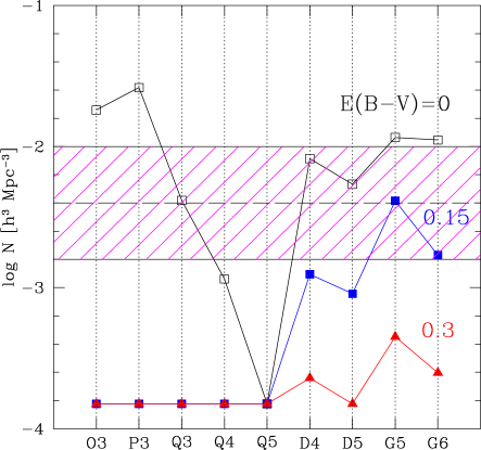
Figure 2: Number density of galaxies for all the runs shown in Figure 1. Three different symbols denote three different values of extinction: $E(B-V)=0.0$ (black open square), 0.15 (blue filled square), and 0.3 (red filled triangle). Points with the same value of $E(B-V)$ are connected to guide the eye. A conservative range of the observed number density of LBGs is shown as the shaded region, with a central value of $4\times 10^{-3}{h}^{3}{\rm Mpc}^{-3}$ (Adelberger et al., 2003). All the cases with zero LBGs are indicated as $N=-3.8$ dex for plotting purposes.

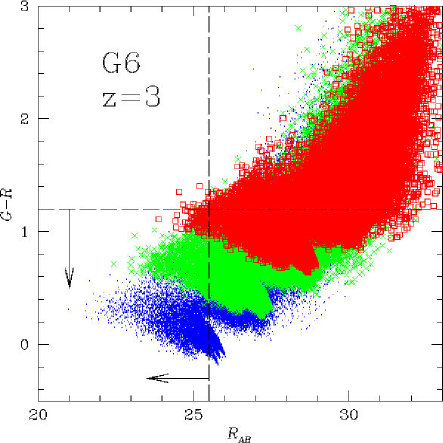
Figure 3: Colour-magnitude diagram for the ‘G6’-run at $z=3$. The distribution of galaxies is shown in the plane of $R$ apparent magnitude and $G-R$ colour. Three different symbols give results for three different values of extinction: $E(B-V)=0.0$ (blue dots), 0.15 (green crosses), and 0.3 (red open squares). The long-dashed lines and the arrow indicate the colour-selection criteria used by Steidel et al. (2003) to identify LBG candidates at $z\sim 3$.

5 Colour-magnitude relation and stellar masses

In Figure 3, we show the distribution of galaxies at $z=3$ in the ‘G6’-run on the plane of $R$-band apparent magnitude and $G-R$ colour. We here chose the ‘G6’-run because it gives a reasonable fit to the observed luminosity functions and the number density, and it has higher resolution than the G5 run. Again, we use three different symbols for three different values of extinction: $E(B-V)=0.0$ (blue dots), 0.15 (green crosses), and 0.3 (red open squares). The long-dashed lines and the arrows indicate the colour-selection criteria applied by Steidel et al. (2003) to select LBG candidates at $z\sim 3$.

We see that most of the galaxies brighter than $R=25.5$ automatically satisfy the criterion $G-R<1.2$, and only a small fraction of galaxies with $R<25.5$ fall out of the region. There is a significant population of dim ($R>28$) galaxies with $G-R>1.2$. We will see below that these are low-mass galaxies with stellar masses $M_{\star}\leq 10^{10}\,h^{-1}{\rm M_{\odot}}$.

In Figure 4, we show the $R$-band apparent magnitude vs. stellar mass of simulated galaxies at $z=3$. As before, we plot results for three values of extinction, using different symbols. We also mark the magnitude limit $R<25.5$ used by Steidel et al. (2003) with a vertical long-dashed line and arrows.

From this Figure, we see that the LBGs in the Q-series with $R<25.5$ have typically stellar masses in the range $M_{\star}=10^{9}-10^{10}\,h^{-1}{\rm M_{\odot}}$, while those in ‘D5’ take a somewhat wider interval, nearly covering the range $10^{8}-10^{11}\,h^{-1}{\rm M_{\odot}}$. The G6 run covers the even wider mass range $M_{\rm star}=10^{8}-10^{12}\,h^{-1}{\rm M_{\odot}}$ depending on the value of extinction. As the wind strength is increased from O3 to P3, and then to Q3-run, we observe that the distribution of galaxies becomes slightly sparser at the most luminous (i.e. massive) end of the distribution. We see the same effect more clearly in the luminosity functions discussed in Section 6. Note that since the numerical resolution is identical for O3, P3, and Q3, the total baryonic mass in the simulation box is the same for these runs, but the runs with stronger winds convert less of their baryonic mass components into stars.

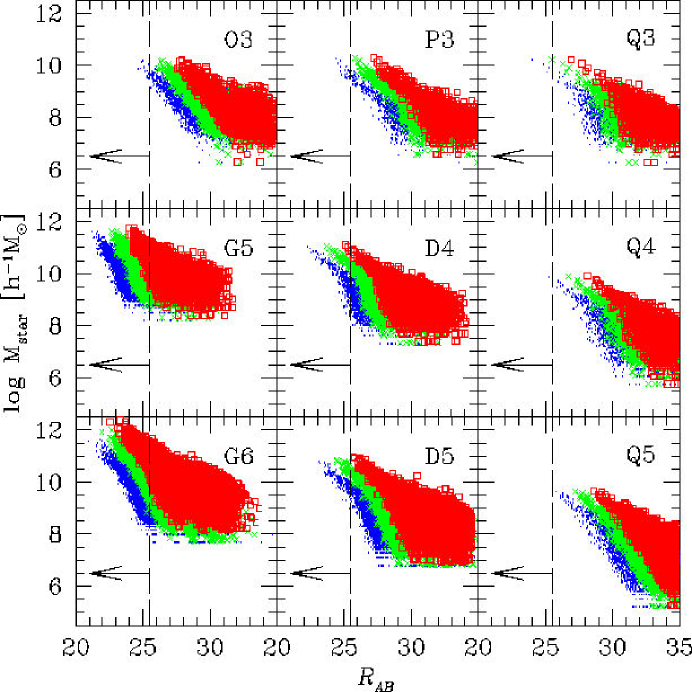
Figure 4: Stellar mass vs. apparent magnitudes of simulated galaxies. Three different symbols are used to show results for three different values of extinction: $E(B-V)=0.0$ (blue dots), 0.15 (green crosses), and 0.3 (red open squares). The vertical long-dashed line and the arrow indicates the magnitude cut used by Steidel et al. (2003).

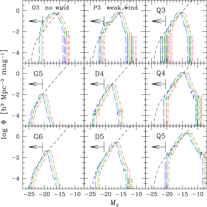
Figure 5: Rest-frame V-band luminosity functions. The three different lines are for three different values of extinction: $E(B-V)=0.0$ (blue long-dashed), 0.15 (green solid), and 0.3 (red dot-dashed). The black short-dashed curve is the observational estimate of the rest-frame V-band luminosity function by Shapley et al. (2001), and the observational magnitude limit of $M_{V}=-20.5$ is shown by the arrows. Note that the Schechter function is plotted down to the fainter magnitudes only to guide the eye for comparison with the simulation results.

In simulations with larger box size (D- and G-series), the masses of the most luminous galaxies found are substantially larger compared with those in the Q-series. This is primarily a result of a finite box size effect; the brightest galaxies have a very low space-density, such that they are simply not found in simulations with too small a volume. On the other hand, the mass resolution of the small box size simulations is much better, so that they can resolve a much larger number of dim low-mass galaxies. Note that the lower cut-off of the distribution in each panel is given by the stellar particle mass of the corresponding simulation.

Interestingly, we find that the amount of stellar mass contained in the LBGs that satisfy the colour selection criteria is in general far from being close to the total stellar mass. In the ‘D5’-run, for example, the LBGs that pass the criteria contain only 20% of all the stars for an extinction of $E(B-V)=0.0$. In the ‘G5’-run, the fraction is 57% and 20% for $E(B-V)=0.0$ and 0.15, respectively. In the ‘G6’-run, the fraction is 52% and 27% for $E(B-V)=0.0$ and 0.15, respectively. This means that the current surveys of LBGs fail to account for more than half of the stellar mass in the Universe. Nagamine et al. (2004) reach a similar conclusion from different theoretical arguments by comparing the results of two different types of hydrodynamic simulations and the theoretical model of Hernquist & Springel (2003) with near-IR observations of galaxies (e.g. Dickinson et al., 2003; Rudnick et al., 2003). Such missed stellar masses might be hidden in the red population of galaxies as suggested by Franx et al. (2003), but in our simulations the missed stellar mass fractions are mainly contained in the faint galaxies below the observational magnitude limit.

6 Luminosity Functions

6.1 Rest-frame V-band luminosity function

In Figure 5, we show the rest-frame V-band luminosity functions for all the simulated galaxies at $z=3$. We have also tried restricting the luminosity functions to only those galaxies that satisfy the colour-selection criteria. Most of the galaxies that fall out of the colour-selection criteria are the less luminous ones as demonstrated in Figure 3. This only affects the faint-end of the luminosity function not probed by current LBG surveys. Therefore we show the luminosity functions for all galaxies in our simulations in Figures 5, 6, & 7 for clarity. As before, we plot results for three different values of extinction: $E(B-V)=0.0$ (blue long-dashed), 0.15 (green solid), and 0.3 (red dot-dashed). Note that stronger extinction simply shifts the luminosity function to the fainter side, without changing its shape. The black short-dashed line included in the figure gives the observational estimate of the rest-frame V-band luminosity function by Shapley et al. (2001) with a faint-end slope of $\alpha=-1.85$, normalisation $\Phi^{*}=0.18\times 10^{-2}h^{3}{\rm Mpc}^{-3}$, and characteristic magnitude $M*=-22.21+5\log h=-22.98$, for $h=0.7$. The observational magnitude limit of $M_{V}=-20.5$ is shown by the arrows.

The most prominent feature seen in all panels is that the luminosity functions of the simulated galaxies are all very steep, with a faint-end slope comparable to $\alpha\sim-2$, which is the slope of the dark matter halo mass function. This suggests that the strong feedback included in the simulations has not been able to reduce the luminosities of low-mass galaxies much more strongly than those of more massive systems; if such a differential effect existed, it should have manifested itself as a flattening of the faint-end compared to the halo mass function. At face value, however, the observational data actually support a rather steep faint-end slope at $z=3$, quite close to that of the halo mass function. One should note, however, that the observational estimate of the slope $\alpha$ at $z=3$ is very uncertain because the observations can only reach down to a magnitude of $M_{V}\sim-20.5$, even with 8-meter class telescopes.

When compared with the observational fit of Shapley et al. (2001), it is clear that the ‘Q’-series are deficient in the brightest galaxies at the high luminosity-end of the luminosity function. This can be understood as a result of the small box size (${L_{\rm box}}=10\,h^{-1}{\rm\,Mpc}$) of these runs, which do not have large enough volume to allow a faithful sampling of rare, bright objects. As the box size becomes larger from the ‘Q’-series to the ‘D’-series (${L_{\rm box}}=33.75\,h^{-1}{\rm\,Mpc}$), and then to the ‘G’-series (${L_{\rm box}}=100\,h^{-1}{\rm\,Mpc}$), this situation improves however. More and more of the luminous objects can then be found, and the agreement with the observation becomes better at the bright-end of the luminosity function.

On the other extreme of the luminosity distribution, we see that increasing the resolution from Q3 to Q4, and then to Q5, allows inclusion of ever fainter objects, as expected. Therefore the luminosity function becomes wider towards the fainter end. Note, however, that the bright-end hardly changes, suggesting good convergence in the simulation results for the massive galaxies.

Figure 6: Comparison of the rest-frame V-band luminosity functions of the O3 (no wind), P3 (weak wind), and Q3 (strong wind) simulations for $E(B-V)=0.3$. The black short-dashed curve is the observational estimate by Shapley et al. (2001), and the observational magnitude limit of $M_{V}=-20.5$ is shown by the arrows. Note that the Schechter function is plotted down to the fainter magnitudes only to guide the eye for comparison with the simulation results.

The run ‘O3’ (no wind run) slightly overpredicts the number of galaxies compared to observations, arguing for the need of stronger feedback. To investigate this further, we explicitly compare in Figure 6 the rest-frame V-band luminosity functions as a function of wind strength. We show the results for the simulations O3 (no wind), P3 (weak wind), and Q3 (strong wind), using an extinction of $E(B-V)=0.3$. For reference, we include the observational estimate by Shapley et al. (2001) as a black short-dashed curve. Clearly, stronger galactic winds reduce the number of bright galaxies, as a result of the suppression of star formation they incur. The same effect has been found in the Eulerian hydrodynamic simulations by Nagamine, Cen, & Ostriker (2004, in preparation).

6.2 Luminosity functions as observed at z=0

In Figure 7, we show the $R$-band luminosity function of simulated $z=3$ galaxies as seen at the present epoch. As in Figure 5, the three different lines are for three different values of extinction: $E(B-V)=0.0$ (blue long-dashed), 0.15 (green solid), and 0.3 (red dot-dashed). The open square symbols give the direct observational result for the luminosity function of LBG galaxies in the observed frame, while the solid circles are the data corrected for dust extinction, as given in Fig. 13 of Adelberger & Steidel (2000). For the uncorrected data points (open squares), a Schechter function fit with parameters $\Phi^{*}=4.4\times 10^{-3}$ $h^{3}{\rm Mpc}^{-3}{\rm mag}^{-1}$, $M^{*}=24.54$, and $\alpha=-1.57$ is also drawn as a short-dashed line. As discussed in Section 3, we applied the Calzetti et al. (2000) extinction law locally at $z=3$ to the simulated galaxies, and then redshifted their spectra, while simultaneously accounting for the absorption by the IGM following the prescription of Madau (1995). The combined effects of redshifting and absorption by the IGM change the shape of the luminosity function in a complex manner compared to the rest-frame.

For the Q-series, the agreement between the simulations and the observational data of Adelberger & Steidel (2000) is not very good. On the bright end, these runs simply lack galaxies due to their small box size, explaining the discrepancy. But the well resolved faint-end appears to show some excess over the observational result. The G-series agrees better with the observations however. In particular, the G5 and G6 runs with $E(B-V)=0.15$ agree well with the uncorrected observed luminosity function, and the case for $E(B-V)=0.0$ is reasonably close to the dust corrected one of Adelberger & Steidel (2000).

Adelberger & Steidel (2000) corrected their observed luminosity function for dust by adopting the relation $A_{1600}=4.43+1.99\beta$ (Meurer, Heckman, & Calzetti, 1999) for the extinction in magnitudes at 1600 Å, where $\beta$ is the UV slope of the spectrum which has a distribution in the range of $[-3,0]$ with a peak around $-1.5$, corresponding to $A_{1600}\sim 1.4$ mag (see Fig. 12 of Adelberger & Steidel, 2000). This peak value is roughly consistent with the value of $E(B-V)=0.15$ we adopted here with the Calzetti et al. (2000) extinction law $k(\lambda)$, because $E(B-V)k(1600\AA)\sim 1.5$ mag. Therefore the rough agreement between the simulated luminosity function with $E(B-V)=0.0$ for G5 and G6-run and the dust corrected data points of Adelberger & Steidel (2000) is encouraging, although not perfect.

Also, note that the peaks of the luminosity functions of the G5 run with $E(B-V)=0.0$ are on the brighter side of $R=25.5$ owing to the lower resolution. This results in the increase of the number density of the LBGs that satisfy the colour-selection criteria when the resolution is increased from the G5 to G6 run as described in Section 4.

Overall, the comparison of the simulated luminosity functions with the observational results presented in Sections 6.1 and 6.1 stresses the importance of having a large simulation box size ($>100h^{-1}{\rm\,Mpc}$) in order to obtain reasonable agreement at the bright end. In our simulations, only the G-series contain a sufficient sample of LBGs brighter than $R=25.5$ with $E(B-V)=0.15$.

7 Star Formation History of LBGs

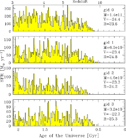
Figure 8: Star formation histories of selected galaxies in the ‘G6’-run with the bin-size of 10 Myrs. Galaxy ID, stellar mass in units of $\,h^{-1}{\rm M_{\odot}}$, rest-frame $V$-band magnitude, and apparent $R$ magnitude for $E(B-V)=0.15$ are indicated in each panel for the corresponding galaxy.

In Figure 8, we show four examples of typical star formation (SF) histories of galaxies in the ‘G6’ run with a bin-size of 10 Myrs, as derived from the age distribution of stars found in each galaxy including all the progenitors that merge prior to $z=3$. We here chose the G6 run because it gives a reasonable agreement with observations both for the $R$-band and rest-frame $V$-band luminosity functions, and it has higher resolution than the G5 run. On the right hand side of each panel, we indicate for each galaxy an ID, its stellar mass in units of $\,h^{-1}{\rm M_{\odot}}$, its apparent $R$ magnitude (for $E(B-V)=0.15$), and its rest-frame $V$-band magnitude.

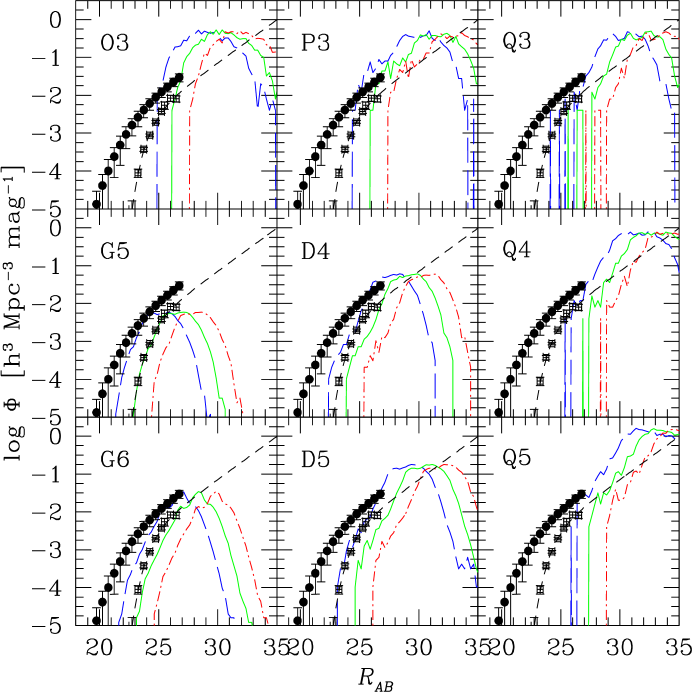
Figure 7: R-band luminosity functions as observed at $z=0$. The three different lines are for three different values of extinction: $E(B-V)=0.0$ (blue long-dashed), 0.15 (green solid), and 0.3 (red dot-dashed). The open square symbols give the observed luminosity function, while the solid circles are the dust corrected data points, as shown in Fig. 13 of Adelberger & Steidel (2000).

A notable feature present in all the panels is the numerous spikes of starbursts lying on top of a relatively continuous component. The starbursts last $10-20$ Myrs, but the underlying smooth component shows only moderate variations in its rate when averaged over bins of 100 Myrs beginning from high redshift ($z\sim 10$) to $z=3$ in these galaxies. For example, the galaxy shown in the top panel, which is one of the most massive galaxies in the G6 run with a stellar mass of $M_{\rm star}=1.4\times 10^{11}\,h^{-1}{\rm M_{\odot}}$ and rest-frame V-band magnitude of $-24.4$, has continuously formed stars from $z=10$ to $z=3$ at a typical rate of $\sim 40~{}\rm M_{\odot}~{}{\rm yr}^{-1}$.

In the other panels, we show galaxies of progressively smaller total mass, with correspondingly lower levels of star formation. Note that the galaxy on the bottom has a stellar mass of only $M_{\star}=3.2\times 10^{10}\,h^{-1}{\rm M_{\odot}}$, yet it still satisfies the colour-colour selection criteria, although its luminosity and star formation rate are substantially smaller compared with the galaxy shown in the top panel. The recent star formation near $z=3$ has helped to bring the brightness of this relatively small mass galaxy above the limit of $R=25.5$.

Interestingly, the underlying continuous component of the star formation histories measured here are much smoother than the ones found by Nagamine (2002) when analysing a Eulerian hydrodynamic simulation. Their starbursts were more extended on the order of 100 Myrs, and more sporadic. This difference is likely related to the different models used by the codes for the treatment of the physics of star formation. In the SPH methodology we investigate here, a sub-resolution multiphase model for the ISM was used which has a self-regulating property; i.e. gas that cools smoothly onto the ISM is also consumed in a smooth fashion by star formation, and only gas-rich major mergers can trigger starbursts.

8 Discussion

We have used state-of-the-art hydrodynamic simulations of structure formation to study the properties of LBGs in a $\Lambda$CDM universe. Our simulations use a new ‘entropy conserving’ SPH formulation that minimises systematic inaccuracies in simulations with cooling, as well as an improved model for the treatment of the multiphase structure of the ISM in the context of star formation and feedback (Springel & Hernquist, 2003a). For the first time, our study uses a large series of simulations to investigate the properties of LBGs, allowing an exploration of an unprecedented large dynamic range in both mass and spatial scales, while simultaneously providing reliable estimates of systematic effects due to numerical resolution.

By comparing our results for LBG properties in simulations with different box size, we showed that a sufficiently large volume (at least ${L_{\rm box}}>50\,h^{-1}{\rm\,Mpc}$) is crucial to faithfully sample the LBG population. In particular, the bright-end of the LBG luminosity function is invariably incomplete in simulations with small box size. Of equal importance is a proper treatment of effective feedback processes. By considering a series of runs with different strengths of galactic winds, we showed that without an effective feedback process, the number of LBGs is overpredicted. However, for our default model of strong winds, a reasonable space density of bright LBGs is obtained. In particular, we found that our G-series with a box size of ${L_{\rm box}}=100\,h^{-1}{\rm\,Mpc}$ has a quite plausible LBG population, with luminosity functions in both rest-frame $V$-band and observed-frame $R$-band that match the observations reasonably well, at least at the bright-end.

Perhaps the most important conclusion of this paper is that the observed properties of LBGs, including their number density, colours, and luminosity functions, can be well explained if the LBGs are simply associated with the most massive galaxies at $z=3$, with median stellar mass of $M_{*}\sim 10^{10}\,h^{-1}{\rm M_{\odot}}$. This conclusion is consistent with earlier numerical studies based on hydrodynamic simulations of the $\Lambda$CDM model (Davé et al., 1999; Katz, Hernquist & Weinberg, 1999; Nagamine, 2002; Weinberg, Hernquist & Katz, 2002) as well as some semi-analytic models (Baugh et al., 1998; Kauffmann et al., 1999), and does not provide direct support for alternative models which suggest that LBGs are star-bursting low-mass systems that later evolve into low-mass spheroids at $z=0$. This point is corroborated by the high rates of star formation with $>10~{}\rm M_{\odot}~{}{\rm yr}^{-1}$ seen over extended periods of time of order 1 Gyr in the simulated galaxies, leading to the build-up of typical stellar masses of $10^{10}\,h^{-1}{\rm M_{\odot}}$ at $z=3$. These comparatively steady star formation histories are also consistent with observational studies by Papovich et al. (2001) and Shapley et al. (2001). Note however that these same observations also find some evidence for starburst activity ($\geq 100\,\rm M_{\odot}{\rm yr}^{-1}$) within the last 500 Myr before $z=3$, lasting for periods of $\sim 100$ Myr. Such long violent bursts are not seen in our SPH simulations, but they were present in the simulations analysed by Nagamine (2002). Instead, multiple shorter bursts with time-scale of $\sim 10-20$ Myr are seen in our SPH simulations.

A recent study by Weatherley & Warren (2003) however claims that the kinematic measurements of Pettini et al. (2001) and Erb et al. (2003) favour the picture of LBGs being low-mass starbursting systems. But the measured ‘rotation curves’ are strongly dependent on seeing, and it is very likely that these measurements underestimate the true rotation curves (M. Pettini, private communication), casting some doubt on these claims. To settle this issue, we have to wait for the detection of a definite flattening of the rotation curves, which might become possible in the near future with near-IR spectrographs coupled to adaptive optics systems. Another difficulty with the low-mass starbursting-galaxy picture for LBGs is that such systems would be expected to have relatively low chemical abundances, whereas at least the brighter LBGs have near-solar metallicity.

The luminosity functions we measure for our simulated LBG galaxies are characterised by a steep faint end, with a slope close to $\alpha\sim-2$. This is the slope of the dark matter halo mass function, so in our simulations, the galaxy luminosity function seems to largely follow the halo mass function at the low-mass end. Observationally, we know that at $z=0$ the faint-end slope of galaxies is certainly much shallower than this, with a slope of order $\alpha\sim-1.2$ (Blanton et al., 2001). At high-redshift, the faint-end of the galaxy luminosity function is not nearly as well constrained, however, and may be much steeper. In fact, Shapley et al. (2001) report a slope of $\alpha=-1.85$ for LBG galaxies at $z=3$ which is still consistent with our simulations. However, as the authors explain, this should be taken with some caution because their observations only reach an absolute $V$-band magnitude of $-20.5$, which is not deep enough to constrain the faint-end slope reliably. If confirmed, a steep luminosity function at $z\simeq 3$ would in any case have to evolve into a much flatter one at low redshift. Whether such a scenario is viable or not will be tested by current and future very deep surveys, such as DEEP2 (Davis et al., 2002; Madgewick et al., 2003; Coil et al., 2003).

Barring confirmation of a rapid evolution of the faint-end slope, our results therefore hint that the simulations still overproduce the number of low-mass galaxies, despite the inclusion of strong feedback processes that are capable of accounting for the observed brightness of $L_{\star}$-galaxies. The moderating effects of feedback on star formation do depend on galaxy mass in the physical model followed by the simulations in the sense that, for a given amount of star formation, the feedback by winds does comparatively more damage for small mass galaxies. This is because towards smaller galaxy mass scales, the winds find it easier to escape from their confining galactic potential wells. The winds also entrain more gas in the outflow for lower circular velocities, so that the net baryonic loss becomes larger towards smaller mass scales, making the total mass-to-light ratio of smaller halos in principle bigger. But, this variation of the feedback efficiency with galaxy mass may not be strong enough in the present set of simulations to close the significant gap between the faint-end slopes of halo mass function and galaxy luminosity function.

Interestingly, the studies by Chiu, Gnedin & Ostriker (2001); Nagamine et al. (2001), and Nagamine (2002) based on Eulerian hydrodynamic simulations did find a flatter faint-end slope (see also Harford & Gnedin, 2003). Presently it is unclear whether this was due to resolution limitations in the low-mass end of the halo mass function, or due to genuine physical effects of the feedback model implemented in these Eulerian simulations. More work in the future will be needed to settle this very interesting question, which is of tremendous importance for the theoretical framework of hierarchical galaxy formation in CDM universes.

References

- Adelberger et al. (2003) Adelberger K. L., Steidel C. C., Shapley A. E., Pettini M., 2003, ApJ, 584, 45