Probing the variability of the fine-structure constant
with the VLT/UVES

We assess the cosmological variability of the fine-structure constant $\alpha$ from the analysis of an ensemble of Fe ii $\lambda 1608$, $\lambda 2344$, $\lambda 2374$, $\lambda 2383$, $\lambda 2587$, and $\lambda 2600$ absorption lines at the redshift $z=1.15$ toward the QSO HE 0515–4414 by means of the standard many-multiplet (MM) technique and its revision based on linear regression (RMM). This is the first time the MM technique is applied to exceptional high-resolution and high signal-to-noise QSO spectra recorded with the UV-Visual Echelle Spectrograph (UVES) at the ESO Very Large Telescope (VLT). Our analysis results in $\langle\Delta\alpha/\alpha\rangle_{\mathrm{MM}}=(0.1\pm 1.7)\cdot 10^{-6}$ and $\langle\Delta\alpha/\alpha\rangle_{\mathrm{RMM}}=(-0.4\pm 1.9\pm 2.7_{\mathrm{sys}})\cdot 10^{-6}$, which are the most stringent bounds hitherto infered from an individual QSO absorption system. Our results support the null hypothesis $\langle\Delta\alpha/\alpha\rangle=0$ at a significance level of 91 percent, whereas the support for the result $\langle\Delta\alpha/\alpha\rangle=-5.7\cdot 10^{-6}$ presented in former MM studies is 12 percent.

1 Introduction

Modern 10 m class telescopes equipped with instruments like the High-Resolution Echelle Spectrograph (HIRES) at the Keck Observatory or the UV-Visual Echelle Spectrograph (UVES) at the ESO Very Large Telescope (VLT) facilitate the accurate observation of QSO absorption (or emission) lines in order to study the hypothetical variability of fundamental physical constants like the fine-structure constant $\alpha=e^{2}/(4\pi\epsilon_{0}\hbar c)$ or the proton-electron mass ratio $\mu=m_{\mathrm{p}}/m_{\mathrm{e}}$. The interest in these studies is motivated by the unification theories incorporating varying fundamental constants (for a review see, e.g., Uzan, 2003).

From the astronomical point of view the cosmological variability of the fine-structure constant is assessed as

$$\Delta\alpha/\alpha=(\alpha_{z}-\alpha_{0})/\alpha_{0},$$ (1)

where $\alpha_{0}$ and $\alpha_{z}$ denote the values of the fine-structure constant in the laboratory and the specific absorption (or emission) line system at redshift $z$, respectively. While observational studies based on the fine-structure splitting of intergalactic alkali-doublet (AD) absorption lines (e.g., Levshakov, 1994; Murphy et al., 2001b) and intrinsic QSO emission line doublets (Bahcall et al., 2003) have provided robust upper bounds on $|\Delta\alpha/\alpha|$, Murphy et al. (2003a, hereafter MFW) have recently detected a non-zero expectation value $\langle\Delta\alpha/\alpha\rangle$ for a sample of 143 complex metal absorption systems identified in QSO spectra recorded with the Keck/HIRES: $\langle\Delta\alpha/\alpha\rangle=(-5.7\pm 1.1)\cdot 10^{-6}$ in the redshift range $0.2<z<4.2$. This remarkable statistical evidence for a cosmological variation of the fine-structure constant is achieved by means of the many-multiplet (MM) technique, which is a generalization of the AD method incorporating the multi-component profile decomposition of many transitions from different multiplets of different ionic species (Dzuba et al., 1999; Murphy et al., 2003b, hereafter MWF, and references therein). While the MM technique considerably improves the formal accuracy, it also shows some immanent deficiencies. Levshakov (2003) illustrates in detail that the prerequisite assumption that the spatial distribution is the same for all ionic species is not valid in typical intergalactic absorption systems. Consequently, it is more reliable to apply the MM technique to samples of absorption lines arising from only one ionic species. Furthermore, in comparison to the AD calculations the incorporation of more transitions over a wider wavelength range results in a stronger susceptibility to systematic effects. Nevertheless, sources of error like wavelength miscalibration, spectrograph temperature variations, atmospheric dispersion, and isotopic or hyperfine-structure effects do demonstrably not explain the detected non-zero expectation value (Murphy et al., 2001a, MWF, MFW). The observational discrepancy grows since the radioactive decay rates of certain long-lived nuclei deduced from geophysical and meteoritic data provide a stringent bound, $\langle\Delta\alpha/\alpha\rangle=(8\pm 8)\cdot 10^{-7}$, back to the epoch of Solar system formation, $z\leq 0.45$ (Olive et al., 2003).

In the optical spectroscopy, the most striking deficiency inherent to all decomposition techniques are non-linear inter-parameter correlations preventing the accurate optimization of the model parameters and possibly causing ambigous results. In fact, the spectral resolution attained in QSO observations at the 10 m class telescopes is still not sufficient to resolve the metal lines with an expected minimum thermal width of about 1 km s^-1. Clearly, in order to solve the profile decomposition problem spectral observations with the highest possible resolution and the highest possible signal-to-noise ratio are desirable.

Table 1: Atomic data of the Fe ii transitions between $\lambda 1608$ and $\lambda 2600$. The laboratory wavelengths $\lambda$, oscillator strengths $f$, and relativistic correction coefficients $q$ are excerpted from MWF Table 2 and Dzuba et al. (2002, Table 1). The sensitivity coefficient $Q$ is defined in Sect. 3.2. Estimiated errors are indicated in parentheses

Tr.	$\lambda$ (Å)	$f$	$\phantom{-}q$ (cm-1)	$\phantom{-}Q$
$1608$	$1608.45080\,(8)$	$0.058$	$-1300\,(300)$	$-0.021\,(5)$
$2344$	$2344.2130\,(1)$	$0.114$	$\phantom{-}1210\,(150)$	$\phantom{-}0.028\,(4)$
$2374$	$2374.4603\,(1)$	$0.0313$	$\phantom{-}1590\,(150)$	$\phantom{-}0.038\,(4)$
$2383$	$2382.7642\,(1)$	$0.320$	$\phantom{-}1460\,(150)$	$\phantom{-}0.035\,(4)$
$2587$	$2586.6496\,(1)$	$0.06918$	$\phantom{-}1490\,(150)$	$\phantom{-}0.039\,(4)$
$2600$	$2600.1725\,(1)$	$0.23878$	$\phantom{-}1330\,(150)$	$\phantom{-}0.035\,(4)$

In this study, we present exceptional high-resolution and high signal-to-noise spectra of the notably bright intermediate redshift QSO HE 0515–4414 (Reimers et al., 1998, $z=1.73$, $B=15.0$) recorded with the VLT/UVES. The spectra reveal a multi-component complex of metal absorption lines associated with a sub-damped Lyman-$\alpha$ (sub-DLA) system at the redshift $z=1.15$ (de la Varga et al., 2000; Quast et al., 2002; Reimers et al., 2003). We analyze a homogenous subsample of Fe ii $\lambda 1608$, $\lambda 2344$, $\lambda 2374$, $\lambda 2383$, $\lambda 2587$, and $\lambda 2600$ absorption lines by means of the standard and a revised MM technique in order to assess the cosmological variability of the fine-structure constant.

2 Observations

HE 0515–4414 was observed with UVES during ten nights between October 7, 2000 and January 3, 2001. Thirteen exposures were made in the dichroic mode using standard settings for the central wavelenghts of 3460/4370 Å in the blue, and 5800/8600 Å in the red. The CCDs were read out in fast mode without binning. Individual exposure times were 3600 and 4500 s, under photometric to clear sky and seeing conditions ranging from 0.47 to 0.70 arcsec. The slit width was 0.8 arcsec providing a spectral resolution of about 55 000 in the blue and slightly less in the red. The ThAr lamp exposures taken immediately after each science exposure provide an accurate calibration in wavelength. The standard deviation of the wavelength versus pixel dispersion solution is about 2.0 mÅ (2.5 mÅ) in the blue (red), resulting in an absolute accuracy of about 0.15 km s^-1 in radial velocity space. The raw data frames were reduced at the ESO Quality Control Garching using the UVES pipeline Data Reduction Software. The calibrated spectra were converted to vacuum wavelengths according to Edlén (1966) while the barycentric velocity correction was manually cross-checked using the ESO-Munich Image Data Analysis Software and the Image Reduction and Analysis Facility. The individual vacuum-barycentric corrected spectra were manually cleaned from cosmic rays or pixel defects, rescaled to a common median flux level, and resampled to an equidistant wavelength grid using natural cubic spline interpolation. The combined spectra (Fig. 1) show an effective signal-to-noise ratio per pixel typically better than 100.

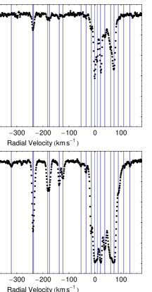
Figure 1: Multi-component Fe ii absorption complex at redshift $z=1.15$. For convenience, only the transitions $\lambda 1608$ and $\lambda 2383$ are shown. Individual components are marked by a vertical line. The zero point of the radial velocity corresponds to the redhsift $z=1.1508$. A close-up ranging from $-20$ to $100$ km s^-1 is provided in Fig. 2

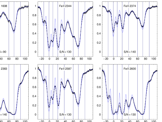
Figure 2: Close-up of Fig. 1 showing the subset of line profiles associated with the central region of the sub-DLA system. The solid and dashed curves represent the optimized model and its deconvolution, respectively. The standard deviation of the normalized flux is indicated by vertical bars whereas the effective signal-to-noise ratio per pixel is stated explicitly. Data marked by empty circles are ignored in the optimization

3 Analysis

3.1 The standard MM technique

The observed spectral flux $F(\lambda)$ is modelled as the product of the background continuum $C(\lambda)$ and the absorption term convoluted with the instrumental profile, i.e., $F(\lambda)=C(\lambda)\int P(\xi)\,\mathrm{e}^{-\tau(\lambda-\xi)}\,\mathrm{d}\xi.$ While the background continuum is locally approximated by an optimized linear combination of Legendre polynomials of up to second order, the instrumental profile is modelled by a normalized Gaussian given by the the spectral resolution of the instrument. Assuming pure Doppler broadening, the optical depth $\tau(\lambda)$ is a superposition of Gaussian functions

$$g_{i}(\lambda)=\frac{e^{2}}{4\epsilon_{0}mc}\frac{N_{i}f_{i}\lambda_{i}}{\sqrt{\pi}b_{i}}\,\exp{\left[-\left(c\,\frac{\lambda-Z_{i}\lambda_{i}}{Z_{i}\lambda_{i}b_{i}}\right)^{2}\right]},$$ (2)

where $Z_{i}=(1+z_{i})(1+u_{i}/c)$ while $\lambda_{i}$, $f_{i}$, $z_{i}$, $u_{i}$, $b_{i}$, and $N_{i}$ denote, respectively, the systemic rest wavelength, the oscillator strength, the cosmological redshift, the radial velocity, the line broadening velocity, and the column density corresponding to the line $i$. The systemic rest wavenumber $\omega_{i}=1/\lambda_{i}$ is parametrized as

$$\omega_{i}=\omega_{0,i}+q_{i}\,(\Delta\alpha/\alpha)\,(2+\Delta\alpha/\alpha),$$ (3)

where $\omega_{0,i}=1/\lambda_{0,i}$ is the wavenumber in the laboratory and $q_{i}$ is the relativistic correction coefficient (Dzuba et al., 2002).

Even though the sub-DLA system exhibits many additional metal absorption lines (Al ii, Al iii, Mg i, Mg ii, Si ii, Cr ii, Ni ii, and Zn ii) typically incorporated in the standard MM analysis, we decide to apply this technique to the Fe ii transitions only. The restriction to one ionic species avoids systematic effects if the spatial distribution is not the same for all species, and reduces systematic effects arising from isotopic line shifts. In addition, the set of Fe ii transitions between $\lambda 1608$ and $\lambda 2600$ already provides a very sensitive combination for probing the variability of the fine-structure constant.

Each absorption component is modelled by a superposition of Doppler profiles with identical radial velocities, widths, and column densities. In addition, the value of $\Delta\alpha/\alpha$ is confined to be the same for all components. In order to find the optimal set of parameter values for both $\tau(\lambda)$ as well as $C(\lambda)$, the weighted sum of residual squares is minimized by means of an evolution strategy (ES) based on the concept of covariance matrix adaption (Hansen et al., 2003). We ignore the ensemble of Fe ii $\lambda 2383$ and $\lambda 2600$ lines associated with the central region of the sub-DLA system since the profiles are saturated and are otherwise overemphasized in the optimization.

3.2 The regression MM (RMM) technique

The standard MM technique can conveniently be revised to avoid the deficiencies pointed out in Sect. 1. In fact, this technique is essentially similar to the method developed by Varshalovich & Levshakov (1993) in order to infer the cosmological variability of the proton-electron mass ratio $\mu$ from the analysis of molecular hydrogen absorption lines. Argueing by analogy (Levshakov, 2003), in the regime $|\Delta\alpha/\alpha|\ll 1$ we obtain the linear approximation

$$z_{i}=z_{\alpha}+\kappa_{\alpha}Q_{i},$$ (4)

where $z_{i}=\lambda_{\mathrm{obs}}/\lambda_{0,i}$ and $Q_{i}=q_{i}/\omega_{0,i}$ denote, respectively, the observed redshift and the sensitivity coefficient corresponding to the line $i$, and the slope parameter $\kappa_{\alpha}$ is given by

$$\kappa_{\alpha}=-2(1+z_{\alpha})\,(\Delta\alpha/\alpha).$$ (5)

If $\Delta\alpha/\alpha$ is non-zero, $z_{i}$ and $Q_{i}$ will be correlated and we will be able to estimate the slope $\kappa_{\alpha}$ and the intercept $z_{\alpha}$ from the linear regression analysis of the position of the line centroids in an absorption component. The accuracy of the regression analysis will be improved, if several absorption line samples are combined. In this case, the regression procedure can be generalized appropriately:

$$\zeta_{i}=(\Delta\alpha/\alpha)\,(Q_{i}-\bar{Q}),$$ (6)

where $\bar{Q}$ denotes the mean sensitivity coefficient of the sample, and $\zeta_{i}=(\bar{z}-z_{i})/[2(1+\bar{z})]$ is the normalized redshift while $\bar{z}$ denotes the mean redshift of an absorption component (in radial velocity space $\zeta_{i}=(\bar{u}-u_{i})/[2(c+\bar{u})]$).

In order to determine the central position of several selected Fe ii lines (see Sect. 4.2) we basically follow the same strategy as described in Sect. 3.1. The only differences are that we do not incorporate Eq. (3) and do not confine the radial velocities to be the same for the lines in the selected components. We point out explicitly that even though we apply a parametric profile decomposition technique to determine the position of the line centroids, the RMM analysis is not tied to any specific modelling technique. In principle, the position of the line centroids can even be determined without doing any modelling at all (cf. Levshakov, 2003). Throughout the analysis we use the atomic data listed in Table 1.

Table 2: Standard MM analysis: optimized values and formal standard deviations of the radial velocity $u$, the line broadening velocity $b$, and the column density $N$ of the 29 components constituting the Fe ii absorption complex. The optimized value of $\langle\Delta\alpha/\alpha\rangle$ is $\langle\Delta\alpha/\alpha\rangle_{\mathrm{MM}}=(0.1\pm 1.7)\cdot 10^{-6}$. The zero point of the radial velocity corresponds to the redshift $z=1.1508$

No.	$\phantom{-}u$ (km s-1)	$b$ (km s-1)	$\log N$ (cm-2)
1	$-534.35\pm 0.07$	$2.07\pm 0.16$	$12.29\pm 0.02$
2	$-530.62\pm 0.44$	$7.26\pm 0.41$	$12.06\pm 0.03$
3	$-510.27\pm 0.18$	$7.92\pm 0.36$	$12.14\pm 0.02$
4	$-494.49\pm 0.16$	$4.86\pm 0.32$	$11.91\pm 0.02$
5	$-471.69\pm 0.12$	$2.99\pm 0.20$	$11.91\pm 0.02$
6	$-448.58\pm 0.38$	$2.21\pm 0.87$	$11.15\pm 0.06$
7	$-416.88\pm 0.08$	$1.76\pm 0.20$	$11.91\pm 0.02$
8	$-403.01\pm 0.16$	$2.19\pm 0.37$	$11.79\pm 0.02$
9	$-393.52\pm 0.10$	$3.39\pm 0.22$	$12.12\pm 0.01$
10	$-375.95\pm 0.16$	$4.38\pm 0.22$	$11.77\pm 0.02$
11	$-321.19\pm 0.30$	$6.98\pm 0.58$	$11.52\pm 0.04$
12	$-239.01\pm 0.08$	$1.66\pm 0.11$	$12.55\pm 0.02$
13	$-235.28\pm 0.16$	$5.15\pm 0.15$	$12.51\pm 0.02$
14	$-182.74\pm 0.45$	$4.02\pm 0.42$	$12.07\pm 0.07$
15	$-175.12\pm 0.47$	$4.92\pm 0.40$	$12.18\pm 0.05$
16	$-137.26\pm 0.10$	$3.11\pm 0.18$	$12.05\pm 0.01$
17	$-123.47\pm 0.14$	$4.47\pm 0.20$	$12.00\pm 0.02$
18	$-53.76\pm 0.38$	$6.04\pm 0.59$	$11.43\pm 0.05$
19	$-34.40\pm 0.21$	$5.81\pm 0.36$	$11.77\pm 0.03$
20	$-14.11\pm 0.09$	$5.09\pm 0.10$	$12.85\pm 0.01$
21	$-1.07\pm 0.05$	$3.76\pm 0.06$	$13.56\pm 0.01$
22	$\phantom{-}8.71\pm 0.06$	$3.46\pm 0.10$	$13.28\pm 0.01$
23	$\phantom{-}22.12\pm 0.04$	$4.53\pm 0.06$	$13.54\pm 0.01$
24	$\phantom{-}37.33\pm 0.08$	$6.04\pm 0.14$	$13.13\pm 0.01$
25	$\phantom{-}59.75\pm 0.16$	$11.3\pm 0.2$	$13.48\pm 0.01$
26	$\phantom{-}72.71\pm 0.06$	$5.69\pm 0.08$	$13.50\pm 0.01$
27	$\phantom{-}88.98\pm 0.24$	$9.16\pm 0.52$	$12.51\pm 0.02$
28	$\phantom{-}110.09\pm 1.44$	$11.4\pm 1.7$	$11.70\pm 0.08$
29	$\phantom{-}134.09\pm 0.43$	$4.08\pm 1.00$	$11.19\pm 0.07$

4 Results and discussion

4.1 Standard MM analysis

The optimized values of the model parameters and the standard deviations provided by the covariance matrix of the ES are listed in Table 2. The decomposition of the Fe ii absorption complex is quite evident (see Figs. 1 and 2). This contrasts with the QSO absorption systems considered in former MM studies where many components are typically unresolved and many line profiles are saturated (see MWF, Figs. 3 and 4). Clearly, the components with the most accurately defined line centroids (No. 1, 12, 20–24, 26) are the most important in the MM analysis. Expectedly, the adequate profile decomposition is reflected in the formal accuracy of the result: $\langle\Delta\alpha/\alpha\rangle_{\mathrm{MM}}=(0.1\pm 1.7)\cdot 10^{-6}$ is the most stringent formal bound hitherto infered from an individual QSO absorption system. The best formal accuracy achieved in former MM analyses (see MWF, Table 3) is exceeded by a factor of about three.

4.2 Regression MM analysis

The optimized central positions of the lines considered in the RMM analysis are listed in Table 3. We do not consider component No. 22 since the central positions of the lines in this component are strongly correlated with those in No. 21 and we ignore component No. 24, because the central position of the Fe ii $\lambda 1608$ line is not accurately defined. The regression line (Fig. 3) indicates no correlation between the relative displacement of the lines, $\zeta$, and the sensitivity coefficient $Q$: $\langle\Delta\alpha/\alpha\rangle_{\mathrm{RMM}}=(-0.4\pm 1.9\pm 2.7_{\mathrm{sys}})\cdot 10^{-6}$, where the statistical errors of $\zeta$ and the estimated errors of $Q$ as well as the systematic uncertainties inherent to the wavelength calibration are propagated by means of Monte Carlo simulation. The coefficient of determination is $r^{2}=0.005$, i.e. only half a percent of the variation among the relative displacement of lines is accounted for by the difference in sensitivity. Consulting the $t$ statistic, the observed data support the null hypothesis $\langle\Delta\alpha/\alpha\rangle=0$ at a significance level of 91 percent, whereas the support for the MFW result $\langle\Delta\alpha/\alpha\rangle=-5.7\cdot 10^{-6}$ is 12 percent.

Table 3: Regression MM analysis: optimized centroid positions (Å) of the Fe ii lines between $\lambda 1608$ and $\lambda 2600$ in the selected absorption components. Formal standard deviations are indicated in parentheses

No.	1608	2344	2374	2383	2587	2600
1	3453.2908 (57)	5032.9469 (24)		5115.7159 (17)	5553.4531 (29)	5582.4812 (19)
12	3456.6993 (39)	5037.9119 (23)	5102.9147 (36)	5120.7677 (21)	5558.9313 (28)	5587.9914 (21)
20	3459.2892 (37)	5041.6969 (25)	5106.7434 (36)	5124.6089 (22)	5563.1057 (30)	5592.1855 (24)
21	3459.4431 (11)	5041.9145 (12)	5106.9734 (12)		5563.3452 (11)
23	3459.7131 (13)	5042.3034 (10)	5107.3695 (16)		5563.7764 (11)
26	3460.2938 (17)	5043.1547 (15)	5108.2272 (21)		5564.7129 (16)

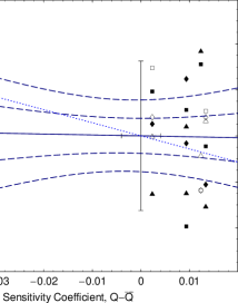
Figure 3: Regression MM analysis of the lines listed in Table 3. Each component is represented by a different symbol. The regression line $\langle\Delta\alpha/\alpha\rangle_{\mathrm{RMM}}=-0.4\cdot 10^{-6}$ and its 68 and 95 percent confidence limits are marked by the solid and dashed curves, respectively, whereas the dotted line indicates the MFW result $\langle\Delta\alpha/\alpha\rangle=-5.7\cdot 10^{-6}$. The median total errors of $\zeta$ and $Q$ are illustrated.

4.3 Systematic effects

Contributing to the discussion of potential systematic effects presented in MWF and MFW, we recall attention to another important source of error. As formerly illustrated by Levshakov & D’Odorico (1995) and Levshakov (1994), the presence of unresolved narrow lines with different optical depths can strongly affect the position of the line centroids in an ensemble of lines and result in a biased expectation value $\langle\Delta\alpha/\alpha\rangle$. This effect will be most noticeable in the case of optically thick lines. In fact, the expectation value $\langle\Delta\alpha/\alpha\rangle_{\mathrm{MM}}$ increases by $3.6\cdot 10^{-6}$ if we do not ignore the ensemble of saturated Fe ii $\lambda 2383$ and $\lambda 2600$ profiles in the optimization, and the systematic increase of scatter in the normalized residuals with increasing optical depth (see Figs. 4 and 5 provided in the online material) may be explained by the presence of unresolved narrow lines.

5 Conclusions

Our results strongly support the null hypothesis of a non-varying fine-structure constant, but do not contradict the MFW result $\langle\Delta\alpha/\alpha\rangle=-5.7\cdot 10^{-6}$ at a significance level higher than $88$ percent. Nevertheless, we conclude: (i) The MM technique has the capability to provide stringent bounds on $\langle\Delta\alpha/\alpha\rangle$ even if the analysis is restricted to the Fe ii lines only. (ii) The RMM technique is illustrative and methodically more transparent than the standard MM technique. In addition, the regression analysis facilitates the consideration of systematic errors inherent to the wavelength calibration of QSO spectra. (iii) The accuracy of the individual $\Delta\alpha/\alpha$ assessment is principally limited by systematic errors inherent to the wavelength calibration. The accuracy attainable with high-quality QSO spectra recorded with the VLT/UVES is limited to $10^{-5}$. (iv) Optically thick profiles are susceptible to systematic effects biasing the expectation value $\langle\Delta\alpha/\alpha\rangle$. (v) The analysis of an extensive homogenous sample of Fe ii absorption lines is inevitable and will provide an independent and crucial test of the MFW result.

In particular, HE 0515–4414 is the brightest known intermediate redshift QSO in the sky and is therefore predestinated for spectroscopy with the new High Accuracy Radial velocity Planet Searcher (HARPS) operated at the ESO La Silla 3.6 m telescope. This very high-resolution spectrograph is specified to provide an efficient wavelength calibration facilitating the performance of radial velocity measurements with an accuracy of better than 1 m s^-1 (Pepe et al., 2002). Presumably, HARPS will improve the accuracy of the individual $\Delta\alpha/\alpha$ assessment by more than an order of magnitude.

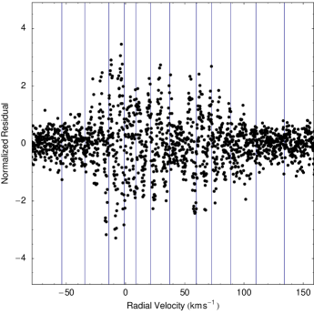
Figure 4: Normalized residuals of the optimized RMM model. For the purpose of residual analysis the calculation of the sum of residual squares takes into account the optically thick parts of the line ensemble. The systematic increase of scatter with increasing optical depth may be explained by the presence of unresolved narrow lines or by deviations from the Doppler profile resulting from e.g. kinematic effects due to rotational motion (Prochaska & Wolfe 1997)

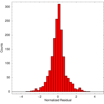
Figure 5: Number distribution of the normalized residuals rendered in Fig. 4. The distribution is approximately normal and does not indicate any missing components