The Distribution of Ly$\alpha$-Emitting Galaxies at z=2.3

Abstract

We present the detection of 34 Ly$\alpha$ emission-line galaxy candidates in a 80$\times$ 80 $\times$ 60 co-moving Mpc region surrounding the known $z=2.38$ galaxy cluster J2143-4423. The space density of Ly$\alpha$ emitters is comparable to that found by Steidel et al. when targeting a cluster at redshift 3.09, but is a factor of $5.8\pm 2.5$ greater than that found by field samples at similar redshifts.

The distribution of these galaxy candidates contains several 5-10 Mpc scale voids. We compare our observations with mock catalogs derived from the VIRGO consortium $\lambda$CDM n-body simulations. Fewer than 1% of the mock catalogues contain voids as large as we observe. Our observations thus tentatively suggest that the galaxy distribution at redshift 2.38 contains larger voids than predicted by current models.

Three of the candidate galaxies and one previously discovered galaxy have the large luminosities and extended morphologies of “Ly$\alpha$ blobs”.

1. Introduction

The two-point correlation coefficient of high redshift ($z>2$) galaxies is quite similar to that of galaxies today (e.g. Steidel et al. 1996, 2000, Giavalisco et al. 1998). The topology of the distribution of high redshift galaxies, however, is not yet clear. The two-point correlation coefficient alone is not very sensitive to this topology. In the local universe, a large fraction of galaxies lie in filaments and sheets, such as the Great Wall (Geller & Huchra 1989). These filaments may be several hundred Mpc in length, and are separated by voids which can be tens of Mpc across. Our understanding of how and when filaments and voids were established depends on the geometry of the universe and biasing of galaxies (e.g. White & Frenk 1991; Kauffmann, Nusser, & Steinmetz 1997; Mo, Mao, & White 1999).

Mapping such large scale structure at high redshifts requires a careful balance of field of view (to encompass the structures), redshift coverage (to accept enough test objects in the structure while avoiding confusion by overlapping structures in distance), and photometric sensitivity (to find enough test objects). Photometric redshifts (see Hogg et al. 1998 for a review) provide an efficient estimate of redshift for large imaging surveys, but they are not accurate enough to avoid confusion from multiple overlapping structures, and cannot delineate the structures directly. Bright QSOs may be markers of dense regions (Ellingson, Yee & Green, 1991), but are too sparse to provide multiple samples within individual structure elements.

Narrow-band imaging to find Ly$\alpha$ emitting galaxies has many advantages as a technique for mapping the topology of the galaxy distribution at high redshifts. The technique picks out galaxies in a narrow-range of redshifts, so the two-dimensional distribution of their positions on the sky can be used to constrain the topology alone, without the need for expensive follow-up spectroscopy. At sufficiently low flux limits the space density of detectable Ly$\alpha$ emitters becomes comparable to that of Lyman-break galaxies (eg. Hu & McMahon 1996). They should be dense tracers of large scale structure. With large-format prime-focus imagers, it is relatively straightforward to survey very large volumes of the early universe. The fast beam required for large field coverage puts a lower limit the width of the narrow-band filter. Typically this limits the line-of-sight depth covered in an exposure to be roughly equal to or greater than the width. A disadvantage of Ly$\alpha$ searches is that the Ly$\alpha$ emission from a galaxy is very hard to predict theoretically, due to the very high optical depth in this line, its dependency on metalicity and star formation rate, and the ease with which it can be obscured by dust.

Two studies find some evidence for filamentary structure in the distribution of Ly$\alpha$ emitting galaxies on scales of around 5Mpc (Campos et al. 1999, Møller & Fynbo 2001). Other surveys have found evidence for clustering in Ly$\alpha$ emitting galaxies, but not for filamentary structure (Steidel et al. 2000, Ouchi et al. 2002).

In this paper, we present the detection of 34 candidate Ly$\alpha$ emitting galaxies in a region containing J2143-4423, a z=2.38 cluster of galaxies and damped Ly$\alpha$ absorbers (Francis et al., 1996, 1997, 2000). Our survey covers a region 80$\times$80$\times$60 co-moving Mpc in size, and hence is sensitive to much larger structures than previous studies at comparable redshifts. The narrow-band imaging also detects four extended nebulae of Ly$\alpha$ emission, often dubbed “blobs” (Steidel et al., 1999, Keel et al. 1999, Francis et al., 2000). Throughout the paper, we assume a $\Lambda$-dominated flat Universe ($H_{0}=65$ km s^-1 Mpc^-1, $\Omega_{M}=0.3,\Omega_{\Lambda}=0.7$).

2. Observations and Data Reduction

The data were taken with the MOSAIC II instrument on the Blanco 4m telescope at CTIO. Observations were made on the nights of 7-8 August, 1999, in the Johnson $UBV$ and Cousins $RI$ filters, and in a custom narrow-band interference filter (NB) centered at 4107Å with a full width at half maximum (FWHM) of 54Å. The NB filter was designed to image Ly$\alpha$ emission at z=2.38 (Francis et al. 2000). The delivered filter covers Ly$\alpha$ redshifts between $2.356<z<2.401$. The Mosaic II is a prime-focus camera consisting of 8 CCDs, each with 2048$\times$4096 pixels. The camera has a plate scale of 0.27″/pixel and covers an overall area of (36′)² with small 9-13″ gaps between the CCDs. Individual exposures were dithered by 10^′. The full NB integration time of 19,800 sec was achieved for a 26′$\times$26′ region centered on the J2143-4423 cluster, while shorter integrations extend over a 48′$\times$50′ field. The final trimmed images are 45.9′$\times$45.5′ in size excluding 9′$\times$9′ in the South-East corner with only one exposure. The observations are summarized in Table 1.

Table 1Observations

Filter	exptime/frame	no. frames	FWHM	$5\sigma$
	(s)		(′′)	(AB mag.)
$U$	1800	5	1.49	23.9
$B$	600	12	1.37	26.2
$V$	600	12	1.37	25.3
$R$	600	5	1.64	24.0
$I$	600	5	1.11	23.8
$NB$	1800,2700	5,4	1.35	23.5

This was the first science run with the MOSAIC II. The readout clocking was still being tuned and biases had a slowly varying harmonic pattern due to the beating of unsynchronized clocks. An FFT based algorithm was developed to subtract the ringing component of the bias. The period of the pattern was approximately 160 pixels (120″) in the readout direction on the CCD. Because this scale is significantly larger than the size of any source in the images the subtraction algorithm should not affect the detection or photometry of of the sources. All detections were verified in the raw images.

Further image reductions were performed using the mscred package in IRAF. These include a correction for crosstalk between the CCDs, bias subtraction and flat-fielding.

Twilight flats were used for all of the images except for the I-band. The I-band twilight flats exhibited considerable fringing with a different pattern than that due to the night sky. The I-band dome flats however were not uniformly illuminated and an illumination correction was derived from highly smoothed twilight flats. The I-band images were defringed by combining all of the images with object rejection. The objects were rejected by making a mask using the SExtractor (Bertin & Arnouts 1996) object images. The object mask images were convolved with a 20 pixel diameter top hat kernel to reject the low surface brightness tails of the objects.

Wide-field optical distortions were corrected using a standard astrometric solution for MOSAIC II provided in IRAF. Final alignment of the images was performed by matching each image to approximately 2000 stars in the APM catalog. The alignment was good to 0.3 pixels (0.08″) rms.

Before combining the images we created bad pixel masks which included hot pixels bad columns and cosmic rays. Cosmic rays were selected using the $jcrrej2$ package in IRAF (Rhoads 2000). We found this package to work extremely well for finding individual cosmic rays, however we had difficulty balancing the parameters to eliminate the faint halos associated with the cosmic ray hits. To eliminate these we devised a filtering algorithm which calculated the Tookey biweight statistic (Beers, Flynn & Gebhardt 1990) in a region around each CR and eliminated all points adjacent to the CR which were $>2.5\sigma$ from the estimated background level.

Photometric calibration was performed using 56 stars in the Landolt fields 90, 92, SA110 and 113 (Landolt 1992). A small correction was include in the calibration to account for Galactic extinction (Schlegel, Finkbeiner & Davis 1998). Catalogs of individual sources were compiled using SExtractor. The limiting magnitudes vary across the images. Figure 1 shows an exposure map for the $NB$ imaging. The map was created by summing a set of the flat field images scaled by exposure times and with the same offsets as the $NB$ exposures. The 5$\sigma$ detection limits for point-like objects in each color are summarized in Table 1. The $NB$ filter was used as a primary detection band, with measurements made in other bands using the same apertures, in order to find objects with weak continua but strong lines. Areas that are covered by only one exposure, such as the south-east corner are excluded from the analysis. Photometry was measured in the Kron aperture (Kron 1980), defined as 2 times the first moment of the radial light distribution. The first moment is approximately equal to the half light radius of the distribution. The photometric error was measured by SExtractor. Table 1 lists the $5\sigma$ photometric sensitivity for a point source in each band.

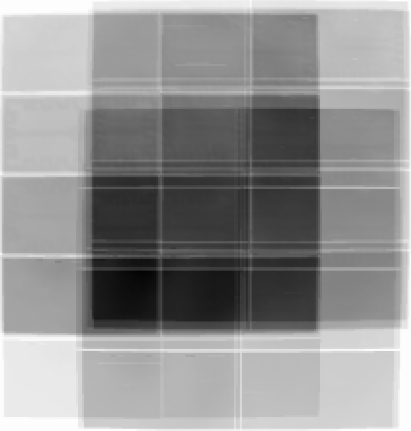
Figure 1.— Exposure map for the $NB$ imaging. North is up East is to the left.

3. Results

We detect 2450 point-like objects and 7000 resolved objects above the $5\sigma$ limit in the NB filter. Ly$\alpha$ emitters can be identified in this sample by excess flux in the NB filter compared to the continuum $B$ filter. The limits for $NB-B$ color excess were determined by modeling the distribution of photometric errors in the $NB-B$ color as a function of the $NB$ magnitude (see Teplitz et al. 1998). The outer envelope of $5\sigma$ errors that defines the detection limit for emission-line candidates is fit by the function:

$$[(NB-15.25)/7.6]^{4}+0.15$$ (1)

However, bright emission-line candidates with low equivalent width (EW) are more likely to be low redshift interlopers than cluster members (see section 3.1). We consider candidates above the $EW=125$ Å limit to be likely Ly$\alpha$ emitters. This limit is obtained as a broad- minus narrow-band color through the relation:

$$NB-B=-2.5\ log{1+EW/W_{B}\over 1+EW/W_{NB}}$$ (2)

where $W_{B}$ and $W_{NB}$ are the widths of the broad- and narrow-band filters.

In addition, objects that are only marginally detected in the narrow-band are unlikely to be good candidates. For simplicity, we establish a uniform narrow-band magnitude cut rather than base the cut on the varying depth across the image. The magnitude cut is based on the 50% completeness limit for narrow-band detections (see Figure 2).

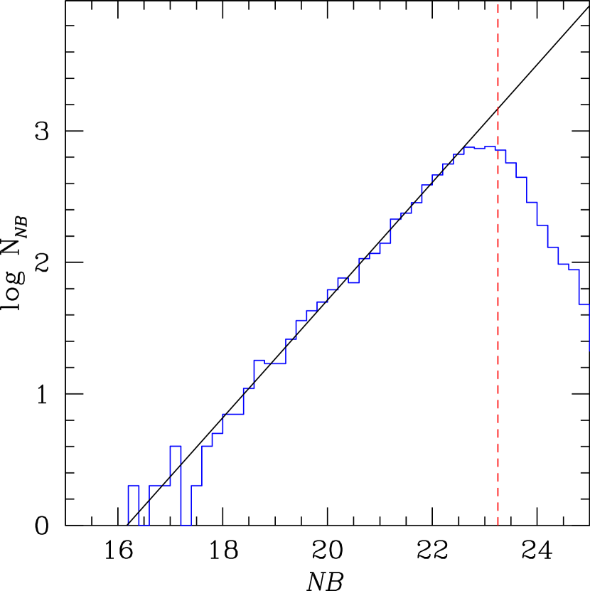
Figure 2.— Number Counts for resolved objects detected in the narrow-band images. Assuming the number counts can be extrapolated by a power law the detections are 50% complete at NB=23.25

Figure 3 shows the $NB-B$ color excess for all objects detected in the $NB$ image. The Ly$\alpha$ emitters from Francis et al. (1996) are clearly detected in the new $NB$ measurement. For new emission line candidates we consider objects that are detected above the 50% completeness limit in the narrow-band filter ($NB<23.5$), are located above the $5\sigma$ color excess line, and have an observed EW greater than 125 Å. We can detect galaxies with emission line strengths brighter than $1.4\times 10^{-16}$ ergs cm^-2 s^-1. This flux limit corresponds to a Ly$\alpha$ luminosity of $1.9\times 10^{9}L_{\sun}$. Thirty-seven spatially resolved $NB$ excess objects are detected. Table 2 lists the positions and measured properties of these objects.

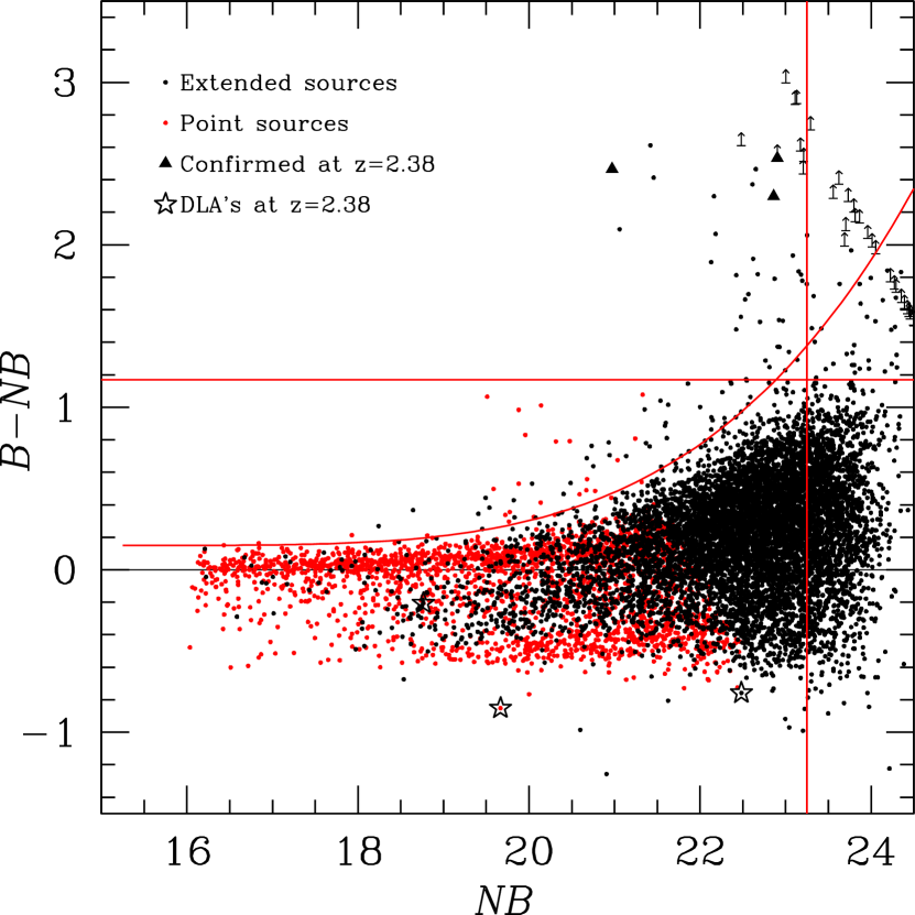
Figure 3.— The excess flux in the NB filter as a function of magnitude. Black points are extended sources and grey are unresolved sources. The large filled circles are the three spectroscopically confirmed Ly$\alpha$-emitters (Francis et al. 1997). Upward pointing arrows are objects undetected in the B-band filter. Three damped Ly$\alpha$ absorbers (Francis & Hewett 1993, Francis, Wilson & Woodgate 2001) are indicated by open stars. The curved lines indicated the $5\sigma$ confidence level for excess emission; that is, points above the line are candidate emission-line object. The horizontal line is the $EW_{obs}=125$ Å level. The vertical line is the 50% completeness cutoff; that is, only candidates brighter than that line are considered likely to be real. Objects which are simultaneously above the $5\sigma$ threshold, above the observed $EW_{obs}=125$ Å level and brighter than the 50% completeness limit are selected as Ly$\alpha$-emission candidates.

Table 2Emission-Line Galaxies

$\alpha$ (2000)	$\delta$ (2000)	$NB$	$B-NB$	Ly$\alpha$ flux	$EW_{0}$	Notes
		(mag.)	(mag.)	($\rm erg~{}cm^{-2}sec^{-1}$)	(Å)
21:40:19.98	-44:19:48.2	22.62	1.91	2.73$\times 10^{-16}$	380
21:40:31.00	-44:36:04.5	22.97	1.53	1.81$\times 10^{-16}$	215
21:40:33.10	-44:36:10.8	22.91	1.37	1.81$\times 10^{-16}$	169
21:40:36.77	-44:20:28.8	23.20	1.78	1.56$\times 10^{-16}$	312
21:40:48.09	-44:31:01.7	23.11	2.87	1.95$\times 10^{-16}$	3026
21:40:48.97	-44:01:23.6	22.77	1.29	2.00$\times 10^{-16}$	150
21:40:58.22	-44:00:22.0	23.00	3.00	2.18$\times 10^{-16}$	5900
21:41:02.90	-44:01:55.9	22.81	1.25	1.89$\times 10^{-16}$	141
21:41:07.38	-44:38:11.7	23.04	1.34	1.59$\times 10^{-16}$	162
21:41:44.41	-44:37:06.7	22.68	1.82	2.54$\times 10^{-16}$	331
21:41:47.66	-44:21:21.9	22.61	2.37	2.95$\times 10^{-16}$	824
21:41:53.55	-44:38:18.3	23.18	1.82	1.60$\times 10^{-16}$	331
21:42:06.03	-44:34:47.9	23.18	2.58	1.79$\times 10^{-16}$	1277	B6
21:42:14.28	-44:32:15.8	22.18	2.07	4.21$\times 10^{-16}$	489
21:42:27.56	-44:20:30.1	20.97	2.47	1.35$\times 10^{-15}$	1004	B1
21:42:28.54	-44:32:38.5	23.20	2.44	1.73$\times 10^{-16}$	944
21:42:29.73	-44:21:02.8	22.86	2.30	2.33$\times 10^{-16}$	723	B2
21:42:32.20	-44:20:18.6	22.90	2.53	2.30$\times 10^{-16}$	1141	B4
21:42:34.88	-44:27:06.2	21.80	3.00	6.95$\times 10^{-16}$	5900	B7
21:42:42.63	-44:30:09.0	21.20	3.00	1.14$\times 10^{-15}$	5900
21:42:54.07	-44:14:39.7	22.93	1.37	1.78$\times 10^{-16}$	169
21:42:56.34	-44:37:56.8	22.48	1.56	2.86$\times 10^{-16}$	225
21:43:00.09	-44:19:21.7	22.57	1.70	2.73$\times 10^{-16}$	277
21:43:03.57	-44:23:44.2	21.42	2.61	9.06$\times 10^{-16}$	1371	B5
21:43:03.80	-44:31:44.9	22.16	2.30	4.43$\times 10^{-16}$	723
21:43:05.90	-44:27:21.0	21.06	2.10	1.19$\times 10^{-15}$	513
21:43:06.42	-44:27:00.6	22.48	2.61	3.41$\times 10^{-16}$	1371
21:43:11.48	-43:59:01.0	23.13	2.87	1.91$\times 10^{-16}$	3026
21:43:22.22	-44:13:06.5	23.09	1.93	1.78$\times 10^{-16}$	392
21:43:23.80	-44:41:36.4	22.87	1.79	2.12$\times 10^{-16}$	317
21:43:24.06	-44:27:59.9	22.42	1.81	3.22$\times 10^{-16}$	326
21:43:37.41	-44:17:53.4	23.21	2.51	1.73$\times 10^{-16}$	1092
21:43:37.48	-44:23:52.8	22.65	2.47	2.88$\times 10^{-16}$	1004
21:43:44.92	-44:05:46.3	22.53	1.66	2.81$\times 10^{-16}$	261
21:43:48.30	-44:08:26.9	22.42	1.48	2.95$\times 10^{-16}$	200
21:44:12.15	-44:05:46.6	21.46	2.41	8.56$\times 10^{-16}$	890
21:44:12.97	-43:57:56.7	22.70	1.53	2.31$\times 10^{-16}$	215

In addition, 7 unresolved objects with $UBV$ colors consistent with QSO’s (e.g., Hall et al. 1996a, 1996b) are detected in emission with equivalent widths greater than 30Å in the observed frame. Table 3 lists the positions and measured properties of these objects.

Finally, a QSO at z=2.38 was found by Hawkins (2000). We detect this object in emission, but it was not selected as a QSO candidate because the $UBV$ colors are within the stellar locus. We include this QSO in Table 3.

Table 3Emission-Line QSO Candidates

$\alpha$ (2000)	$\delta$ (2000)	$NB$	$B-NB$	line flux	$EW_{0}$	$B-V$	$U-B$	Notes
		(mag.)	(mag.)	($\rm erg~{}cm^{-2}sec^{-1}$)	(Å)	(mag.)	(mag.)
21:40:52.46	-44:36:21.35	19.96	0.83	2.04e-15	70	0.26	-0.28
21:41:54.50	-44:18:35.97	20.14	1.01	1.96e-15	96	0.05	-0.31	z=1.66
21:42:35.12	-44:32:30.36	21.35	0.99	6.35e-16	93	0.36	-0.11
21:42:43.49	-44:14:25.32	20.14	0.41	1.02e-15	27	0.07	-0.35
21:43:16.44	-44:16:51.54	21.04	0.67	6.51e-16	51	0.08	-0.30
21:43:20.38	-44:20:00.35	20.59	0.46	7.39e-16	31	0.06	-0.52
21:43:22.53	-44:31:49.18	19.88	0.98	2.45e-15	91	0.04	-0.43
21:43:26.25	-44:26:03.44	20.77	0.49	6.58e-16	34	0.26	-0.33

3.1. Foreground Contamination

For spatially resolved narrow-band excess sources the only likely contaminating line is [O II] (3727Å). Our narrow-band filter centered at 4107Å, is sensitive to [O II] emission from foreground $0.095<z<0.109$ galaxies. Indeed, we detect emission from many well resolved spiral galaxies below our EW cutoff.

[O II] interlopers within our Ly$\alpha$ sample would have absolute B magnitudes around $-13.8$, and would hence be Blue Compact/HII galaxies (BCGs). At this redshift they would only be marginally spatially resolved, so we could not separate them from $z=2.38$ Ly$\alpha$ emitters by morphology alone.

To be detected through our filter, they must lie within a box of comoving size 5.9$\times$5.9$\times$60 Mpc, and have a rest-frame [O II] equivalent width greater than 114Å. Using the local luminosity function of Jerjen, Bingelli & Freeman (2000) we would expect to find $\sim 12$ BCG galaxies in such a box. Pustilnik et al. (1999), however, found that only $\sim 8$% of BCG galaxies have [O II] equivalent widths large enough to meet our selection criteria. If this foreground region was an average one, we would therefore expect $\sim 1$ foreground BCG galaxy to be contaminating our sample.

The southernmost 80% of our field was included in the Las Campanas Redshift Survey (LCRS, Shectman et al. 1996), which has excellent sensitivity to large scale structures at redshift $z\sim 0.1$. The region in which foreground [O II] emitters could contaminate our survey contains a single isolated cluster (Abell 3800, Abell, Corwin & Olowin 1989), but is otherwise empty of galaxies. The LCRS detects many filaments of galaxies at this redshift, but none lie in our field at redshifts that could cause [O II] emission to impersonate Ly$\alpha$ at z=2.38. Despite the presence of Abell 3800, the galaxy density is indeed slightly below the LCRS average at this redshift. Abell 3800 is located 10′ west and 3′ south of our field center (see Fig 4). We see no concentration of candidate Ly$\alpha$ emitting galaxies at this location: indeed quite the opposite. Only one of our candidates lies within one projected Mpc of this location. Three others lie around 1.3 projected Mpc from the cluster, but these are the three for which we have spectroscopic confirmation that they lie at $z=2.38$. We therefore tentatively conclude that foreground contamination is unlikely to be a big problem.

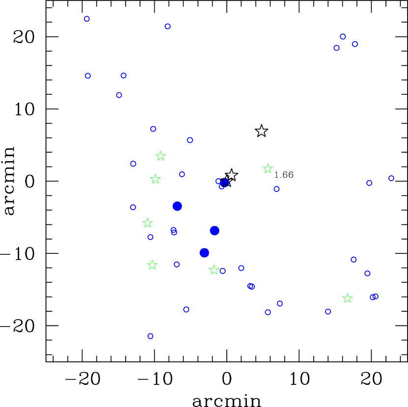
Figure 4.— The distribution of emission-line objects in the field. The small open circles represent emission-line galaxy candidates. The large filled circles are extended emission-line nebulae (blobs). The large open stars are the three known DLAs, and the small open stars are quasar candidates at the cluster redshift or lower redshifts. East is to the left and North is upwards.

Foreground contamination is more likely a problem for the 7 narrow-band excess QSO candidates. The narrow-band excess could be caused by Ly$\alpha$ emission at redshift 2.38, but could also be quasars at other redshifts, with different lines producing the excess. Indeed one of these sources was found (Francis et al. 1997) to be a QSO at z=1.66, with its C IV (1549Å) emission producing the narrow-band excess. The luminosity and redshift distribution of QSOs implies that about 60% or 4 of these quasars should be Ly$\alpha$ emitters at redshift 2.38 (see Palunas et al. 2001). If some of these sources are QSOs at redshift 2.38, it will be further evidence that QSOs lie in the most massive dark matter halos, which in turn exist in the most highly clustered environments (e.g. Silk & Weinberg 1991).

4. Discussion

4.1. The Space Density of Ly$\alpha$ Emitters

We are sensitive to Ly$\alpha$ emitting galaxies over a 45′$\times$45′ field minus 9′$\times$9′in the South-East corner, in the redshift range $2.356<z<2.401$. For our adopted cosmology, this corresponds to a volume 6100 co-moving Mpc² in area and 59 co-moving Mpc deep. Figure 5 shows the density contours of Ly$\alpha$ candidates estimated using an adaptive kernel routine (Beers, Flynn & Gebhardt 1990). The initial smoothing scale is 12 arcminutes. The highest density contour is $5.7\times 10^{-2}$ sources per square arcminute corresponding to a spatial density of $3.0\times 10^{-4}$ sources per cubic Mpc. The average density over the whole field is $1.9\times 10^{-2}$ sources per square arcminute corresponding to a spatial density of $1\times 10^{-4}$ sources per cubic Mpc.

Figure 5.— Density contours for the distribution of Ly$\alpha$ candidates estimated with the adaptive kernel routine. The lowest contour is one galaxy per resolution element $3.3\times 10^{-3}$ galaxies arcmin^-2. The highest contour is $5.7\times 10^{-2}$ galaxies arcmin^-2.

Steidel et al. (2000) surveyed 20,000 cubic co-moving Mpc at redshift 3.09, targeting a cluster of Ly-dropout galaxies. Their survey was sensitive to lower Ly$\alpha$ luminosities than ours, and they used a lower rest-frame equivalent width threshold. They find 9 candidates meeting our luminosity and equivalent width thresholds corrected for redshift, yielding a density of $4.5\times 10^{-4}$ sources per cubic Mpc. Steidel et al. calculate that this space density is a factor of $6.0\pm 2.4$ greater than that of smaller survey of Cowie & Hu (1998). This implies that peak density in our field is a factor of 4 overdense.

4.2. Star Formation Rates

To estimate the star formation rate we first assume that star formation powers the observed Ly$\alpha$ flux. This is almost certainly a great underestimate: even tiny amounts of dust will greatly reduce the observed Ly$\alpha$ flux due to its high optical depth. We use an un-reddened Ly$\alpha$/H$\alpha$ ratio of 8:1, and the conversion factor between H$\alpha$ flux and star formation rate of Kennicutt (1983). Our faintest candidates (NB=23.25) have inferred star formation rates of $\sim 9M_{\sun}{\rm yr}^{-1}$.

Summing over all galaxies down to our flux limit, and making a crude correction for incompleteness amongst the faintest, the integrated star formation rate density (assuming no dust obscuration) is $2.4\times 10^{-3}M_{\sun}{\rm Mpc}^{-3}{\rm yr}^{-1}$: well below the value ($\sim 0.1M_{\sun}{\rm Mpc}^{-3}{\rm yr}^{-1}$) derived from integrated blue light by Madau, Pozzetti & Dickinson (1998).

We also estimate star formation rate from the 1600Å UV continuum using the Madau et al. formula. At z=2.38 the 1600Å continuum falls in the $V$-band. We detect 23 of our candidates in the V-band. The star-formation density implied by these candidates is $5\times 10^{-3}M_{\sun}{\rm Mpc}^{-3}{\rm yr}^{-1}$. The star formation rate for a candidate at the V-band limit of 25.3mag is $\sim 18M_{\sun}{\rm yr}^{-1}$. The 14 galaxies not detected in the $V$-band could add, as an upper limit, $0.6\times 10^{-3}M_{\sun}{\rm Mpc}^{-3}{\rm yr}^{-1}$ to the star formation rate density.

Our Ly$\alpha$ candidates therefore contribute only a small fraction ($\sim 5\%$) of the overall star formation rate density at z=2.38.

In a detailed study of the spectra of Lyman-break galaxies, Shapley et al. (2003) conclude that galaxies with the strongest Ly$\alpha$ emission have bluer UV continua, weaker interstellar absorption and smaller star-formation rates than galaxies with weak Ly$\alpha$ emission or Ly$\alpha$ absorption. Ly$\alpha$ emission from galaxies with the highest star-formation rates is absorbed by dust.

4.3. The Distribution of Ly$\alpha$ Emission Candidates

The distribution of our candidate resolved Ly$\alpha$ emitting sources is shown in Fig 4. There is no obvious overdensity surrounding the previously known cluster at the field center. Instead, most of the candidates lie in a broad band extending from the north-east of the field to the south. There is a significant is the lack of galaxies in the north and west. These regions have long integration times. There are three close pairs or triplets of candidates, but otherwise the candidates are well spaced. The pairs have a spacing of about 20 arcsec or a minimum separation of 200 proper kpc. The spacing of the galaxies in the triplet is about 50 arcsec or a minimum separation of 440 proper kpc.

4.3.1 Comparison to a random distribution

We used two statistics to compare our data to a random distribution. We compare these statistics to results from Monte Carlo simulations generated with the same exposure-time mask. In this section we show that the distribution of our candidates has a significant excess of close ($<1$′) pairs, and of large (6′ – 8′) voids.

The first statistic is essentially the angular two-point correlation function. For a series of angular separations, we take each data point in turn and count the number of other data points within that angular radius.

The second statistic is a two-dimensional analogue of the void probability function (VPF). For each angular scale, we randomly place 1000 circles with that radius on our field, so that the circles do not extend beyond the edge of our data. We count the fraction of these circles which did not contain any data points. The requirement that the circles not extend beyond the edge of the data makes this statistic most sensitive to voids near the center of the field. Void probability functions are sensitive to structures such as voids and filaments, to which the two-point correlation function is relatively insensitive.

Our data were compared to random Monte Carlo simulations generated as follows. At each location in our image, the total exposure time was calculated. Using these total exposure times, the relative flux limits in every part of our field were computed. The number/magnitude distribution of our brighter candidates can be reasonably approximated as a power-law, with the number per unit magnitude increasing by a factor of roughly 5. Combining this number-magnitude relation with the flux limits, we calculated the relative probability of finding a candidate per unit area in any given part of our image. We then used this relative probability map to generate 2000 fake data sets, each containing the same number of sources as in the real data.

Our data have a significant excess of galaxies with separations less than 1′. Only 0.1% of the Monte Carlo simulations produced this many close galaxies. On larger scales, our data still show an excess of galaxies, but this is no longer significant at the 5% level.

The void probability function (Fig 6) is more interesting. There is a clear excess of voids on scales of 5 arcminutes or greater. On scales of 5′ – 8′, this excess is significant at the 99.9% confidence level (ie. fewer than 0.1% of our randomly generated data sets had VPFs as large as our data).

Figure 6.— The void probability function of our data (solid triangles) compared to the average void probability functions of randomly distributed points (solid line) and void probability functions derived from the $\lambda$CDM n-body simulations (open squares).

We conclude that there is a significant excess of voids, and of small scale clustering, in our data. This conclusion is insensitive to the details of how we generated the random data sets: changes in (for example) the assumed number/magnitude relation made little difference to our results.

4.3.2 Comparison with $\lambda$CDM n-body Simulations

The distribution of our Ly$\alpha$ candidates is thus inconsistent with a random distribution, with 99.5% confidence. Assuming that they are indeed galaxies at redshift 2.38, is their distribution consistent with theoretical predictions? In this section, we show that while the two-point correlation coefficient of our galaxy candidates is quite consistent with the predictions of a $\lambda$CDM simulation, the distribution of our candidates shows more voids on 6′ – 8′ scales, with 97% confidence.

To evaluate the apparent excess of voids, we compared our measured distribution of galaxies against the $\lambda$CDM n-body simulations performed by the VIRGO consortium (Kauffmann et al. 1999). We used their galaxy catalog, generated for redshift 2.12. For each galaxy, they list its position, stellar mass, gaseous mass and star formation rate.

Mock catalogs were generated as follows. Our observations were targeted at the source B1, a probable pair of giant elliptical galaxies surrounded by an extensive neutral hydrogen cloud (Francis et al. 2000). B1 has an estimated stellar mass of $10^{10.9}M_{\sun}$ and gaseous mass of $10^{9.7}M_{\sun}$. We picked five galaxies in the $\lambda$CDM simulations that had stellar and gaseous masses at least this large, and which lay far enough from the edge of the simulation volume. The regions around these “B1-analogue” galaxies should be good matches to our data. For comparison, we also picked eight random locations within the $\lambda$CDM simulation volume. We then extracted the galaxies that lay within a volume 70$\times$70$\times$46 co-moving Mpc (for our adopted cosmology) centered at each of these locations. There were $180\pm 30$ (1 $\sigma$) galaxies in their catalogs in each of these volumes.

We then had to sparsely sample the galaxies within each of these volumes to generate mock catalogs with (a) 37 galaxies, and (b) a probability of being detected consistent with our exposure-time map. We did this in three different ways.

1. Randomly. As Ly$\alpha$ emission can be generated in many ways (by star formation, shocks, cooling flows, AGN etc), and its escape in measurable quantities depends on accidents of the geometry and dust distribution inside galaxies, we first assumed that all the galaxies in the $\lambda$CDM simulations had the same probability (37/180 $\sim$ 20%) of being detected by our survey.

2. Star Formation Rate. If the Ly$\alpha$ flux is generated by star formation, only galaxies with star formation rates in excess of $8M_{\sun}{\rm yr}^{-1}$ would have been detected. We therefore took only galaxies with star formation rates at least this large, and generated random sub-samples with the correct size and probability of detection as a function of position in our field. Only 25% of the galaxies within the $\lambda$CDM cubes had star formation rates this large.

3. Mass. We took only galaxies with masses greater than $10^{10.3}M_{\sun}$, once again picking random sub-samples of the appropriate size and with probabilities of detection scaling appropriately with exposure time in each part of our image.

For each data cube, and for each of these three sub-sampling techniques, we repeated the random sub-sampling 2000 times. We then calculated the angular two-point correlation function and the void probability function for each sub-sampling of each data cube, and compared our results with the observations.

Fig 7 shows our data, and five of the mock $\lambda$CDM data cubes (centered on the five B1-analogue galaxies). The cubes shown have been randomly sub-sampled: those sampled on the basis of star formation rate or mass look very similar. Fig 6 shows the average void probability function of the randomly sub-sampled data cubes (centered on B1-analogue galaxies).

Figure 7.— The distribution on the sky or our candidate Ly$\alpha$emitting galaxies (top left) compared to five simulated data sets drawn from the $\lambda$CDM n-body simulations. These simulations use random sub-sampling and are centered on B1-analogue galaxies.

The angular two-point correlation coefficient of our data, and of the $\lambda$CDM simulations are in excellent agreement. As Fig 6 shows, however, the agreement is not as good for the void probability function. Our data have a void probability function considerably higher than that of the simulations on large scales.

Is this difference significant? The VPFs of our 13 simulated data cubes (five centered on B1-analogue galaxies and eight randomly located) actually showed rather little scatter, when averaged over all the 2000 random sub-samplings of each. The dominant source of scatter was the selection of the 37 galaxies in each simulated volume, which was typically twice as large. Our uncertainty is thus dominated by the small sample size rather than by cosmic variance.

If we take the five data cubes centered on B1-analogues, and generate 2000 random sub-samplings of each, fewer that 0.1% of all these random sub-samplings have void probability functions as large as we observe on scales of 5′ – 8′. If we sub-sample on the basis of star formation rate or galaxy mass, this fraction rises to around 1%. We would expect this, as more massive galaxies, and those with larger star formation rates, are expected to be more strongly biased. If we repeat these calculations for the randomly centered data cubes, the void probability function also rises slightly. This is presumably because centering our data cube on a B1 analogue precludes the possibility of a void in the center of the field.

Thus the observed distribution of galaxies has an excess of voids over the $\lambda$CDM simulations, significant at roughly the 99% level. A qualitative impression of this can be gained from Fig 7. While all the $\lambda$CDM simulations show empty regions near the edge of the field, this is an artifact of the shorter exposure times in these regions. The simulations do not show large voids in the central $\pm 13$ arcminutes. Due to the restriction that we only place voids so that they do not overlap the edges of our field, our VPF statistic is mostly sensitive to the distribution of galaxies in this central region.

4.3.3 Discussion of the Voids

We thus have tentative evidence from our survey of larger voids in the galaxy distribution at redshift 2.38 than predicted by one particular $\lambda$CDM simulation. With only 97% confidence, a sample size of 34 and no spectral confirmation for most of our candidate galaxies, this evidence must be regarded as tentative at best. But if it is confirmed by larger samples, what is it telling us?

Steidel et al. (2000) did not see voids, but they covered too small a region on the sky to be sensitive to the scales of void we are detecting. Ouchi et al. (2003) imaged a region $\sim 25$% the size of ours, searching for Ly$\alpha$ candidates at $z=4.86$. Voids can be seen in their data if only brightest objects are selected so that their number per unit area matches ours. Voids might also explain the enormous field-to-field variance in the space density of Ly$\alpha$ sources found by Pascarelle, Windhorst & Keel (1998). The spiky distribution of the redshifts of Lyman-dropout galaxies seen by Steidel et al. (1998) and Adelberger et al. (1998) would also be consistent with large voids in the high redshift galaxy distribution.

If the distribution of galaxies really contains more 10 co-moving Mpc scale voids than predicted, either $\lambda$CDM is predicting too uniform a distribution of galaxies, or the voids contain dark matter halos which for some reason do not contain detectable galaxies.

There is some evidence for the latter hypothesis. The sight-line to background QSO 2138$-$4427 passes through one of the voids in our data, but the QSO spectrum shows a metal enriched damped Ly$\alpha$ absorption-system at our redshift (Francis & Hewett 1993, Francis, Wilson & Woodgate 2001). So there is clearly at least one dense concentration of gas and some stars within one of our voids.

4.4. Blobs

Some high redshift galaxy clusters contain extended Ly$\alpha$ emission nebulae, or “blobs” (Steidel et al. 1999). The blobs are radio quiet ($<140~{}\mu$Jy at 1.4 GHz), but otherwise share morphological similarity with the nebulae around radio galaxies (e.g. Kurk et al. 2001). Ly$\alpha$ blobs are large, bright gas clouds ($\sim 100h^{-1}$ kpc, $\Omega_{m}=0.3,\Omega_{\Lambda}=0.7$; Ly$\alpha$ flux up to $1.8\times\sim 10^{-15}$ erg cm^-2 s^-1). They appear to be common in regions of significant galaxy overdensity ($\sim 10$ times that of the field) at high redshift. Most blobs are associated with a host galaxy, though not symmetrically centered on it. Blobs may break into smaller knots of Ly$\alpha$ and continuum emission, with velocity differences $\Delta V\mathrel{\hbox to0.0pt{\lower 3.0pt\hbox{$\mathchar 536\relax$}\hss}\raise 2.0pt\hbox{$\mathchar 316\relax$}}2000$ km s^-1 (Steidel et al. 2000). Blobs can be among the brightest high-$z$ sub-mm sources (Chapman et al. 2001). Some blobs (Francis et al. 2001) show CIV emission (and may host AGN) but others do not.

We detect four Ly$\alpha$ blobs in the narrow-band image. One of these, “B1”, has previously been detected (Francis et al. 2001). Figure 8 shows the broad- and narrow-band images of each blob, together with the continuum subtracted emission-line image. Each blob conforms to the expected size and brightness of this class of object. Table 4 summarizes the characteristics of the blobs.

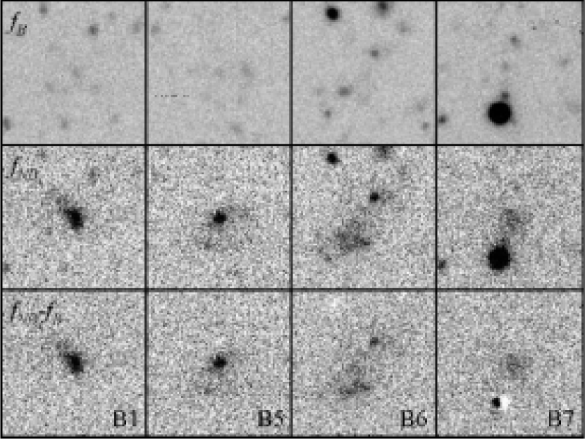
Figure 8.— REDUCED RESOLUTION. Images of the blobs. The top row shows the broad band image of each blob; the middle row the narrow-band image; and the bottom row the difference of the two, scaled to give an image of the Ly$\alpha$ emission. Each image is $30{{}^{\prime\prime}}\times 30{{}^{\prime\prime}}$.

Table 4Ly$\alpha$ Blobs

Name	Redshift	major axis	Ly$\alpha$ flux	CIV emission	Ref.
	($z$)	(′′)	($\rm erg~{}cm^{-2}sec^{-1}$)
SB-1	3.09	17	$1.4\times 10^{-15}$	no	1,2
SB-2	3.09	15	$1.2\times 10^{-15}$	no	1,2
KB-A	2.39	$\sim$8	$1.1\times 10^{-15}$	yes	3,4
KB-B	2.39	$\sim$8	$0.45\times 10^{-15}$	yes	3,4
B1	2.38	17	$1.8\times 10^{-15}$	yes	5, this work
B5	2.38	8	$1.5\times 10^{-15}$	$\cdots$	this work
B6	2.38	8	$1.4\times 10^{-15}$	$\cdots$	this work
B7	2.38	7	$0.7\times 10^{-15}$	$\cdots$	this work

These blobs may be pre-galactic clouds of gas, in the process of initial collapse or destined to be stripped away into the intracluster medium (ICM). In the blobs, we may witness a stage of structure formation which is illuminated by an unusual or transitory phenomenon. The excitation mechanism for the Ly$\alpha$ emission is not known, but three primary models have been suggested:

In the early stages of a galaxy’s formation, gas collapses into the dark matter potential well and cools via radiation (e.g. Fabian et al. 1986). Haiman, Spaans & Quataert (2000) calculate that cooling flows (with gas temperatures of a few $\times 10^{4}$ K) could produce the observed flux range, size, surface brightness profiles and number density observed from Ly$\alpha$ blobs. While Fardal et al. (2000) doubt that cooling flows would have sufficient luminosity, Francis et al. (2001) suggest that shocks within the infalling gas can trigger the blob emission in the cooling flow. Confirmation that the blobs are high redshift cooling flows would have profound implications for the interpretation of semianalytic galaxy formation models (e.g. Fall & Efstathiou 1980) since we would be observing the initial collapse of gas into dark matter potential wells.

Taniguchi et al. (2001 and references therein) suggest that starburst-powered winds trigger Ly$\alpha$ emission in the expelled gas. Dust could obscure the host galaxy, with the Ly$\alpha$ emission arising from a superwind extending $\sim 100$ kpc from the host. The dusty host galaxies would eventually evolve into ordinary elliptical galaxies, and the blobs would presumably dissipate into the intracluster medium. The SCUBA detections support this model, implying rapid star formation (Chapman et al. 2001) and a probability of hosting an AGN (Barger et al. 2001). Superwinds would indicate that the blobs are the next phase of galaxy evolution after the initial collapse. Taniguchi & Shioya (2000) estimate this phase would last only 0.1 Gyr, occurring after the first 0.5 Gyr of star formation. The expelled gas would eventually be stripped into the ICM, though it would be metal-enriched having been processed by supernovae in the host galaxy.

An AGN may photo-ionize the gas, similar to radio galaxy nebulae and Seyfert 2 galaxies with extended emission line regions (e.g. Villar-Martin, Tadhunter & Clark 1997). For example, a Ly$\alpha$ nebula has been found around the HDF-S QSO which is radio-quiet (Bergeron et al. 1999; Palunas et al. 2000a). For the blobs, we do not see a strong UV continuum source; however, there may be an AGN surrounded by an obscuring torus (e.g. Krolik & Begelman 1986). In fact, most of the Chandra point sources do not show optical evidence for AGN (Mushotzky et al. 2000). Assuming an ionization parameter of 10 and a density of 1 cm^-3 at a distance of 10 kpc, a central source with luminosity $9\times 10^{45}$ ergs s^-1 is required to ionize a Ly$\alpha$ blob with $L_{x}\sim 10^{44}$ ergs s^-1. The gas in AGN-supported blobs would contribute to the ICM, but with potentially lower metallicity than that from a starburst, thus diluting rather than enriching the ICM.

5. Summary

Narrow-band imaging in the J2143-4423 region has revealed 34 candidate Ly$\alpha$ emitters, including three new extended Ly$\alpha$ blob candidates and five possible quasars. Together with the previously reported emission-line galaxies and DLA systems, these detections suggest this field is one of the most highly evolved structures detected at high redshift.

The distribution of the candidates is non-random. There are more closely grouped galaxies, and more voids in the distribution, than would be expected from either a random distribution of galaxies or from the $\lambda$CDM simulations of Kauffmann et al. (1999). This may indicate some environmental dependence on whether a galaxy emits detectable Ly$\alpha$ emission.

The detection of too many voids in our data is suggestive, but further observations with much more uniform sensitivity over much wider fields, combined with follow-up spectroscopy, will be required to definitively measure the topology of the distribution of high redshift galaxies.

References

- (1)
- (2) Abell, G. O., Corwin, H. G., & Olowin, R. P. 1989, ApJS, 70, 1
- (3)
- (4) Adelberger, K. L., Steidel, C. C., Giavalisco, M., Dickinson, M., Pettini, M., & Kellogg, M. 1998, ApJ, 505, 18
- (5)
- (6) Barger, A. J., Cowie, L. L., Mushotzky, R. F., & Richards, E. A. 2001, AJ, 121, 662
- (7)
- (8) Bautz, M. W., & Garmire, G. P. 2001, AAS, 199, 100.10
- (9)
- (10) Beers, T. C., Flynn, K., & Gebhardt, K. 1990, AJ, 100, 32
- (11)
- (12) Bergeron, J., Petitjean, P., Cristiani, S., Arnouts, S., Bresolin, F., & Fasano, G. 1999, A&A, 343, L40
- (13)
- (14) Bertin, E., & Arnouts, S. 1996, A&AS, 117, 393
- (15)
- (16) Campos, A., Yahil, A., Windhorst, R. A., Richards, E. A., Pascarelle, S., Impey, C., & Petry, C. 1999, ApJL, 511, L4
- (17)
- (18) Chapman, S. C., Lewis, G. F., Scott, D., Richards, E., Borys, C., Steidel, C. C., Adelberger, K. L., & Shapley, A. E. 2001, ApJ, 548, L17
- (19)
- (20) Cowie, L. L., & Hu, E. M. 1998, AJ, 115, 1319
- (21)
- (22) Ellingson, E., Yee, H. K. C., & Green, R. F. 1991, ApJ, 371, 49
- (23)
- (24) Fabian, A. C., Arnaud, K. A., Nulsen, P. E. J., & Mushotzky, R. F. 1986, ApJ, 305, 9
- (25)
- (26) Fall, S. M., & Efstathiou, G. 1980, MNRAS, 193, 189
- (27)
- (28) Fardal, M. A., Katz, N., Gardner, J. P., Hernquist, L., Weinberg, D. H., & Davé, R. 2001, ApJ, 562, 605
- (29)
- (30) Francis, P. J., & Hewett, P. C. 1993, AJ, 105, 1633
- (31)
- (32) Francis, P. J., et al. 1996, ApJ, 457, 490
- (33)
- (34) Francis, P. J., Woodgate, B. E., & Danks, A. C. 1997, ApJ, 482, L25
- (35) Francis, P. J., Wilson, G. M., & Woodgate, B. E. 2001, PASA, 18, 64
- (36)
- (37) Francis, P. J., et al. 2001, ApJ, 554, 1001
- (38)
- (39) Geller, M. J., & Huchra, J. P. 1989, Science, 246, 897
- (40)
- (41) Giavalisco, M., Steidel, C. C., Adelberger, K. L., Dickinson, M. E., Pettini, M., & Kellogg, M. 1998, ApJ, 503, 543
- (42)
- (43) Haiman, Z., Spaans, M., & Quataert, E. 2000, ApJ, 537, L5
- (44)
- (45) Hall, P. B., Osmer, P. S., Green, R. F., Porter, A. C., & Warren, S. J. 1996a, ApJ, 462, 614
- (46)
- (47) Hall, P. B., Osmer, P. S., Green, R. F., Porter, A. C., & Warren, S. J. 1996b, ApJ, 471, 1073
- (48)
- (49) Hawkins, M. R. S. 2000, A&AS, 143, 465
- (50)
- (51) Hogg, D. W. et al. 1998, AJ, 115, 1418
- (52)
- (53) Hu, E. M., & McMahon, R. G. 1996, Nature, 382, 281
- (54)
- (55) Jerjen, H., Bingelli, B., & Freeman, K. C. 2000, AJ, 119, 593
- (56)
- (57) Kauffmann, G., Nusser, A., & Steinmetz, M. 1997, MNRAS, 286, 795
- (58)
- (59) Kauffmann, G., Colberg, J. M., Diaferio, A., & White, S. D. M. 1999, MNRAS ,303, 188
- (60)
- (61) Keel, W. C., Cohen, S. H., Windhorst, R. A., & Waddington, I. 1999, AJ, 118, 2547
- (62)
- (63) Kennicutt, R. C., Jr. 1983, ApJ, 272, 54
- (64)
- (65) Krolik, J. H., & Begelman, M. C. 1986, ApJ, 308, L55
- (66)
- (67) Kron, R. G. 1980, ApJS, 43, 305
- (68)
- (69) Kurk, J. D., Pentericci, L., Røttgering, H. J. A., & Miley, G. K. 2001, ApSSS, 277, 543
- (70)
- (71) Landolt, A. U. 1992, AJ, 104, 340
- (72)
- (73) Le Févre, O., Deltorn, J. N., Crampton, D., & Dickinson, M. 1996, ApJ., 471, L11
- (74)
- (75) Lowenthal, J. D., Hogan, C. J., Green, R. F., Caulet, A., Woodgate, B. E., Brown, L., & Foltz, C. B. 1991, ApJ, 377, L73
- (76)
- (77) Madau, P., Pozzetti, L., & Dickinson, M. 1998, ApJ, 498, 106
- (78)
- (79) Mo, H. J., Mau, S., & White, S. D. M. 1999, MNRAS, 304, 175
- (80)
- (81) Møller, P., & Fynbo, J. U. 2001, A& A, 372, L57
- (82)
- (83) Mushotzky, R. F., Cowie, L. L., Barger, A. J., & Arnaud, K. A. 2000, Nature, 404, 459
- (84)
- (85) Ouchi, M. et al. 2003, ApJ, 582, 60O
- (86)
- (87) Pascarelle, S. M., Windhorst, R. A., & Keel, W. C. 1998, AJ, 116, 2659
- (88)
- (89) Pascarelle, S. M., Windhorst, R. A., Keel, W. C., & Odewahn, S. C. 1996, Nature, 383, 45
- (90)
- (91) Palunas, P., et al. 2000, ApJ, 541, 61
- (92)
- (93) Pritchet, C. J. 1994, PASP, 106, 1052
- (94)
- (95) Pustilnik, S. A., Engels, D., Ugryumov, A. V., Lipovetsky, V. A., Hagen, H.-J., Kniazev, A. Y., Izotov, Y. I., & Richter, G. 1999, A & AS, 137, 299
- (96)
- (97) Rhoads, J. E. 2000, PASP, 112, 703
- (98)
- (99) Shapley, A. E., Steidel, C. C., Pettini, M., & Adelberger, K. L. 2003, ApJ, 588, 65
- (100)
- (101) Schlegel, D. J., Finkbeiner, D. P., & Davis, M. 1998, ApJ, 500, 525
- (102)
- (103) Shectman, S. A., Landy, S. D., Oemler, A., Tucker, D. L., Huan, L., Kirshner, R. P., & Schechter, P. L. 1996, ApJ, 470, 172
- (104)
- (105) Silk, J. & Weinberg, D. 1991, Nature, 350, 272
- (106)
- (107) Steidel, C. C., Giavalisco, M., Pettini, M., Dickinson, M., & Adelberger, K. L. 1996, ApJ Letters 462, L17
- (108)
- (109) Steidel, C. C., Adelberger, K. L., Dickinson, M., Giavalisco, M., Pettini, M., & Kellogg, M. 1998, ApJ, 492, 428
- (110)
- (111) Steidel, C. C., Adelberger, K. L., Shapley, A. E., Pettini, M., Dickinson, M., & Giavalisco, M. 2000, ApJ, 532, 170
- (112)
- (113) Taniguchi, Y., & Shioya, Y. 2000, ApJ, 532, L13
- (114)
- (115) Taniguchi, Y., Shioya, Y., & Kakazu, Y. 2001, ApJ, 562, L15
- (116)
- (117) Teplitz, H. I, Malkan, M. A., & McLean, I. S. 1998, ApJ, 506, 519
- (118)
- (119) Villar-Martin, M., Tadhunter, C., & Clark, N. 1997, A& A, 323, 21
- (120)
- (121) White, S. D. M., & Frenk, C. 1991, ApJ, 379, 52
- (122)
- (123) Windhorst, R. A., Keel, W. C., & Pascarelle, S. M. 1998, ApJ, 494, L27
- (124)