Reconstructing the Peak Distribution in the Sunyaev-Zeldovich Effect Surveys

Abstract

We examine the ability of the Sunyaev-Zel’dovich effect (SZE) statistics proposed by Lee (2002) using numerical simulations. The statistics describe the distribution of the peak heights in the noise-contaminated SZE sky maps, and provide an analysis technique to sort out the noise-contamination effect and estimate the number density of real clusters. The method is devised to be suitable for the interferometric SZE observations in drift-scanning mode like AMiBA experiment. We apply the proposed method to a set of realistic SZE sky maps constructed from large-scale cosmological simulations, and show that the method indeed allows us to estimate the number density of clusters efficiently. The efficiency of the method is demonstrated in two aspects: (i) it can reconstruct the number density of clusters even though the clusters contribute only a small fraction ($\sim 10\%$) of the total number of peaks in each SZE map; (ii) it can count even those clusters whose amplitudes are low enough to be compatible with the noise level while conventional method of cluster identification using the threshold cutoff cannot count them properly within the same observation time. Thus, the proposed method may be useful for the study of cluster abundance exploiting future interferometric SZE surveys such as AMiBA.

1 INTRODUCTION

The thermal Sunyaev-Zel’dovich effect (SZE) by galaxy clusters represents the spectral distortion of the cosmic microwave background radiation (CMBR) through the inverse Compton scattering by the hot intra-cluster electrons (Sunyaev & Zel’dovich, 1972). Since the SZE is independent of the redshift, it provides a unique tool to detect high-redshift clusters. Thus, the blank-field SZE survey can measure the formation epoch and the abundance evolution of galaxy clusters, which can be used as a probe to put constraints on the cosmological parameters (Barbosa et al., 1996; Henry, 1997; Bahcall & Fan, 1998; Viana & Liddle, 1999; Borgani et al., 1999; Fan & Chiueh, 2001; Grego et al., 2001; Molnar et al., 2002).

The SZE flux diminution is directly proportional to the cluster Comptonization parameter $y$, defined as

$$y(\vec{\theta})=\frac{\sigma_{T}k_{B}}{m_{e}c^{2}}\int n_{e}(l\hat{\theta})T_{e}(l\hat{\theta})dl,$$ (1)

where $\vec{\theta}$ represents the location vector along the line-of-sight ($\hat{\theta}\equiv\vec{\theta}/|\vec{\theta}|$) and the integral is over the CMBR path in the line-of-sight direction. Hence the SZE survey at a fixed frequency basically provides a map of the $y$-parameter. The number density of galaxy clusters, however, cannot be directly measured from the observed SZE maps because of the presence of noise.

Conventionally, signals from the noise-contaminated maps are identified as the local peaks whose flux amplitudes (for the SZE observation, proportional to the peak height of the Comptonization parameter, $y$) significantly exceed the noise level. Therefore, to detect lower-amplitude signals using the conventional approach, one has to decrease the noise level by increasing the observational time. Unfortunately, the necessary observational time increases inversely proportional to the squares of the imposed noise level. It is clearly inefficient to use the conventional signal-selection method for the estimate of the cluster number counts, because of the high costs of the interferometric observations.

Recently Lee (2002) proposed a statistical strategy to estimate efficiently the number density of galaxy clusters from the noise-contaminated SZE maps constructed from the interferometric observation in drift-scanning mode, with the AMiBA experiment as a target model. By the efficient estimate, we mean that the method is capable of estimating the number density of clusters which contribute only a small fraction of the total number density of peaks in the SZE maps, counting properly even those clusters whose peak heights are low enough to be compatible with the noise level without increasing the observational time. The key feature of the method is to exploit the property that the noise-contamination is described by a Gaussian statistic. Then the cluster number density can be estimated by simply deconvolving a one-dimensional Gaussian function and the zero-th order approximation to the cluster number density. Although the method has been shown to render reasonable results for idealized Monte-Carlo simulations (Lee, 2002), it is necessary to test its ability by applying it to more realistic simulations before using it in real SZE surveys.

In this Letter, we test the ability of the SZE statistical strategy using the outputs of a large cosmological simulation. In $\S 2$, we provide a concise overview of the model experiment AMiBA and the SZE statistics. In $\S 3$, we describe the numerical simulation, explain how to apply the statistical strategy to the simulated SZE maps, and compare the reconstructed cluster number densities with the original ones. In $\S 4$, we summarize the results, and give concluding remarks.

2 The SZE CLUSTER SURVEY

2.1 AMiBA in a Drift-Scan Mode

For the blank-field SZE survey, we have two types of observations: the single dish bolometric observations such as BOLOCAM (Glenn et al., 1998) and the multiple dish interferometric observations such as our model experiment, AMiBA (Lo et al., 2000). AMiBA (Array for Microwave Background Anisotropy) is an interferometer telescope with $19$ dishes of $1.2$ meter, dedicated to SZE observation at operating frequency of $90\pm 16$ GHz. It is designed to be most suitable for a deep survey of low-mass clusters at high redshifts. For this purpose, it has relatively small beam of $2$ arcminute, and plans to survey $5$ square degree for 20 hours per field on average (the total period is over $7$ months), expected to be able to detect $1$ cluster per every $9$ hour.

An observational strategy of AMiBA is to use the drift-scan method, which will help keep the ground fringes constant with time, improve the Fourier-space resolution, and most importantly simplify the noise analysis (Pen et al., 2002). A drift-scanned sky map from AMiBA experiment will be a combination of a small fraction of cluster signals ($\sim 10\%$) and a large fraction of dominant instrumental noise. The distribution of cluster signals is non-Gaussian, while that of the instrumental noise is Gaussian with no spatial correlation. Since the statistical property of a Gaussian field is well known, the noise analysis for the SZE sky maps from AMiBA experiment in drift-scanning mode may be analytically tractable (Zhang et al., 2002; Lee, 2002).

2.2 The SZE Statistics : An Overview

The peak number density of a Gaussian random field is analytically given by (Longuet-Higgins, 1957; Bond & Efstathiou, 1987):

$$n_{g}(\nu)=\frac{1}{(2\pi)^{3/2}}R_{*}^{-2}e^{-\frac{\nu^{2}}{2}}\int^{\infty}_{0}[x^{2}+e^{-x^{2}}-1]\frac{\exp[-\frac{1}{2}(x-\gamma\nu)^{2}/(1-\gamma^{2})]}{[2\pi(1-\gamma^{2})]^{1/2}}dx,$$ (2)

where $\nu$ is the peak height rescaled by the noise dispersion, $\sigma_{0}$, $\sigma^{2}_{i}=\frac{1}{(2\pi)^{2}}\int|W(u)|^{2}u^{2i}d^{2}{\bf u}$ with a noise filter $W(u)$, $R_{*}\equiv\sqrt{2}(\sigma_{1}/\sigma_{2})$, and $\gamma\equiv\sigma_{1}^{2}/(\sigma_{0}\sigma_{2})$. Equation (2) implies that the number density of the Gaussian noise is a sharply decreasing function of $\nu$, which in turn suggests that the noise effect will be almost completely negligible for very high signals $\nu>5$.

The presence of noise contaminates the SZE sky map, making it obscure to count the number density of true signal peaks in many different ways: it changes the amplitudes and locations of the signal peaks, and also it creates or compromises signal peaks. To make matters worse, the fraction of the signal peaks is usually only a few ten percent of the noise peaks. Lee (2002) suggested, however, that all the various noise-contamination effects on the number density of real clusters $n_{cl}(y)$ could be quantified by a one-dimensional Gaussian distribution with the unit dispersion $p(x)=(1/\sqrt{2\pi})e^{-x^{2}/2}$, and that $n_{cl}(y)$ be statistically estimated by deconvolving $p(x)$ and the zeroth-order approximation to the cluster number density $n^{(0)}_{cl}(y)\equiv n_{sz}(y)-n_{g}(y)$ where $n_{sz}(y)$ is the number density of local peaks in a SZE map:

$$n_{cl}^{(0)}(y)=\frac{N_{cl}^{\rm tot}}{N_{sz}^{\rm tot}}\int p(x)n_{cl}(y-x)dx,$$ (3)

where $N_{sz}^{\rm tot}$ and $N_{cl}^{\rm tot}$ are the total number of local peaks in a SZE map and that of real clusters, respectively.

The stabilized deconvolution of $p(x)$ and $n^{(0)}_{cl}(y)$ can be performed in the Fourier space as

$$\tilde{n}_{cl}(y_{k})=\frac{W_{p}(y_{k})\tilde{n}^{(0)}_{cl}(y_{k})}{\tilde{p}(y_{k})},$$ (4)

where $y_{k}$, $\tilde{n}_{cl}$, $\tilde{n}^{(0)}_{cl}$, and $\tilde{p}$ are the Fourier counter parts of $y$, $n_{cl}$, $n^{(0)}_{cl}$, and $p$, respectively. Here, $W_{p}(y_{k})$ represents the Wiener optimal filter (Press et al., 1992), a key quantity to the deconvolution process. It is introduced to stabilize the process of the deconvolution on a discretized mesh. The functional form of $W_{p}(y_{k})$ is determined from the power spectrum of the $y$-peaks; the ratio of the true power spectrum ($P_{-}$) to the measured one ($P_{+}$). The measured power spectrum $P_{+}$ is usually a corrupted one due to the numerical noise effect. The true power spectrum $P_{-}$ is supposed to be well estimated by subtracting the obvious noise tail from the measured power spectrum $P_{+}$ (see Fig. 2). Finally, the inverse Fourier transform of $\tilde{n}_{cl}(y_{k})$ gives the desired estimate of the cluster number density $n_{cl}(y)$.

The validity and stability of the above statistical method depends on the heights of $y$-peaks considering the definitions of $n^{(0)}_{cl}(y)$ and $p(x)$. In the very low $y$ range where the noise peaks are dominant (say, $y<\sigma^{N}$, where $\sigma_{N}$ is the noise level), $n^{(0)}_{cl}(y)$ is close to zero, and hence the deconvolution likely fails. In other words, in the low $y$ range, most of the local peaks can be safely regarded as just noise. Also, in the very high $y$ range (say, $y>5\sigma_{N}$) where the signal peaks are dominant, we have $n^{(0)}_{cl}(y)\approx n_{sz}(y)\approx n_{cl}(y)$. In this range the noise contamination effect is almost completely negligible so that the deconvolution of $p(x)$ is not meaningful any longer. Hence it is naturally expected that the above statistical method works best in the range of medium $y$ peaks (say, $\sigma_{N}<y\leq 5\sigma_{N}$) where $n^{(0)}_{cl}(y)$ has non-zero values while containing a substantial noise-contamination that can be quantified as $p(x)$. We emphasize that it is this range of $\sigma_{N}<y\leq 5\sigma_{N}$ where we hope to estimate the cluster number density more efficiently than the conventional method.

3 APPLICATION TO NUMERICAL SIMULATIONS

We use the SZE cluster catalogues produced from a large cosmological simulation carried out by the Virgo consortium (Jenkins et al., 2001; Yoshida et al., 2001). We make maps of $2048^{2}$ pixels in a field of view of 3.14 degree on a side. Details of the generation of the SZE cluster maps are found in Yoshida (2002). For our purpose, we use a total of 8 realizations of the SZE cluster maps, each of which corresponds to a patch of the SZE sky map. We first smooth the SZE cluster maps by a Gaussian filter of scale radius $R_{g}$ in order to mimic the diffuse and extended clusters observed in real surveys. The scale radius $R_{g}$ corresponds to the FWHM (full-width at half maximum) of the clusters which varies with different observations. Here we choose $R_{g}=2$ arcminute, given that the natural beam is expected to have a FWHM of $2$ arcminute in AMiBA experiment. Next, we construct a Gaussian random field on the same $2048^{2}$ pixels using the Monte-Carlo method, assuming the flat-sky approximation. To simulate the instrumental noise of the real SZE observation, we adopt a white-noise power spectrum as the random field, and then convolve it with the noise-cleaning filter $W_{C}$ which is given in Fourier ${\bf u}$-space (${\bf u}$: the Fourier counterpart of $\vec{\theta}$, $u\equiv|{\bf u}|$) as (Pen et al., 2002; Lee, 2002):

$$W_{C}(u)=\frac{1}{u}\left[\exp\left(-\frac{u^{2}\theta^{2}_{A}}{2}\right)-\exp\left(-\frac{u^{2}\theta^{2}_{B}}{2}\right)\right],$$ (5)

where $\theta_{B}=6\theta_{A}$ with $\theta_{A}=0.5$ arcminute suitable for AMiBA (Pen 2002, private communication). For each of the 8 realizations of SZE cluster maps, we construct an independent noise field, and combine the cluster sources with the noise field to construct a realistic, noise-added SZE map. In combining, we rescale each field by the y-dispersion of the noise, $\sigma_{y}^{N}$. Figure 1 shows one realization of the sky maps of original SZE clusters (the top panel) and its smoothed version combined with the noise field (the bottom panel), respectively. From each realization of the total SZE map, we determine the number density of the peaks $n_{sz}$ as a function of the rescaled peak heights. Using the measured $n_{sz}$ along with equation (2), we compute the zero-th approximation to the cluster number density, $n^{(0)}_{cl}$, and measure the power spectrum of the peaks from the total SZE map in order to find a Wiener optimal filter $W_{p}$. Figure 2 shows an example of the peak power spectrum computed from one realization. The solid line corresponds to the measured power spectrum $P_{+}$ from the total SZE map realization, revealing the noise tail. The dashed line represents the estimate of the true power spectrum $P_{-}$, obtained by subtracting the noise tail from $P_{+}$. The Wiener optimal filter for the deconvolution is then approximated as $P_{-}/P_{+}$.

Finally, by using this Wiener optimal filter, we perform the stabilized deconvolution of the zero-th order signal distribution $n_{cl}^{(0)}$ and the one-dimensional Gaussian distribution $p(x)$ to estimate the true number density of the signal peaks. We found that for all realizations our method works quite well in the range of $\sigma_{y}^{N}<y\leq 5\sigma_{y}^{N}$ within a $\sim 25\%$ error. Figure 3 plots the number counts of local peaks per degree square as a cumulative function of the rescaled Comptonization parameter $N_{cl}(\geq y)\equiv\int_{y}n_{cl}(y^{\prime})dy^{\prime}$ for the case of each realization separately. The long-dashed, the dotted, and the solid lines represent the cumulative number densities of local peaks from the total SZE map, noise peaks from equation (2), and the signal peaks from the reconstruction, respectively, while the square dots represent the cumulative number densities of signals from the original SZE simulations before the noise contamination effect added. Figure 4 plots the same as Figure 3 but averaged over all 8 realizations. Our method reconstructs also the averaged peak distribution fairly well.

4 SUMMARY AND CONCLUSIONS

We have tested the validity of the SZE statistics proposed by Lee (2002) using numerical simulations. The statistical method is devised for the interferometric SZE observations in drift scanning mode, targeting at AMiBA as a model experiment, and applied to estimate the number density of cluster signals that occupy only a small fraction ($\sim 10\%$) of the noise-contaminated SZE maps more efficiently than the conventional method based on the threshold cut-off. The method is developed to model the dominant noise contamination effect on the SZE peak distribution by a Gaussian scatter and to deconvolve the noise scatter and the SZE peak distribution. The stability of the deconvolution process has been achieved by convolution with a Wiener optimal filter estimated from the measurable power spectrum of the SZE peaks.

We have applied the method to a large number of realistic SZE sky maps, and found that it indeed works for all realizations, giving a fairly good estimate of the cluster number density, including even those clusters whose peak heights are compatible with noise-levels. In the conventional approach, those low-amplitude peaks are usually all disregarded as noise, so that a large fraction of low-amplitude cluster signals are missing. Our method allows us to count those missing low-amplitude clusters as quickly and accurately as possible. Hence, we conclude that it will provide an efficient method to determine the number density of galaxy clusters in the future interferometric SZE surveys.

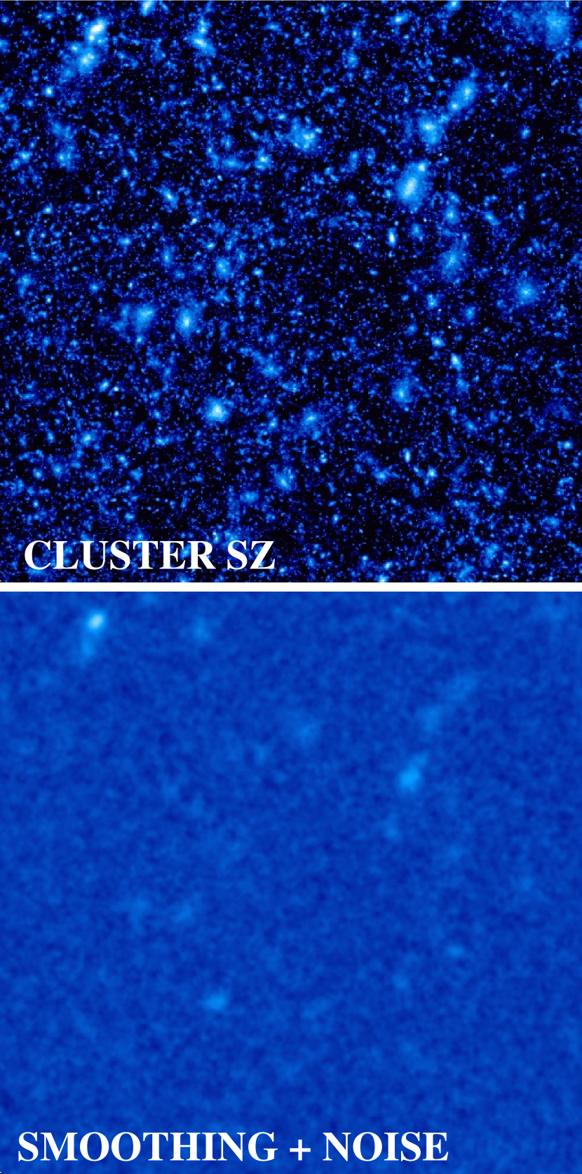
Figure 1: Simulated thermal SZ effect maps. The maps shows the same field of view of 3.14 degree on a side. Top: a pure thermal SZ effect; Bottom: a smoothed SZE map combined with a Gaussian noise field (see $\S 3$ in text).

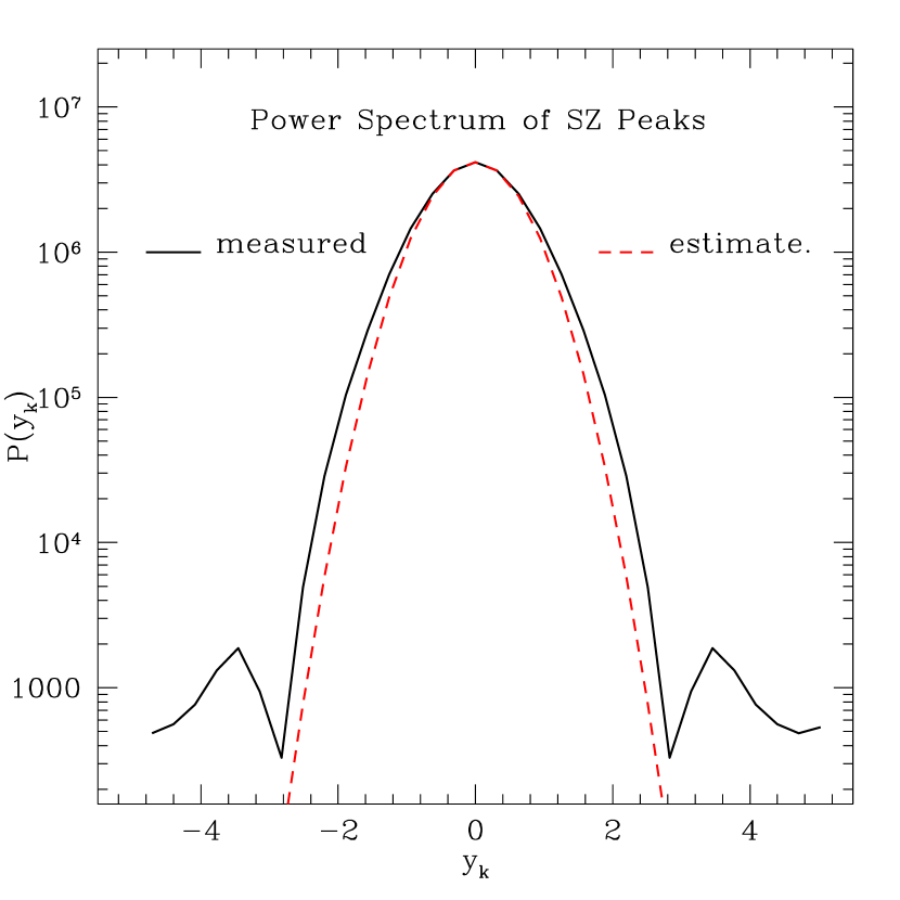
Figure 2: The power spectrum of the rescaled $y$-peaks measured from one realization of the total SZE map. The solid line is the measured power spectrum, while the dashed line represents our estimate of the true power spectrum.

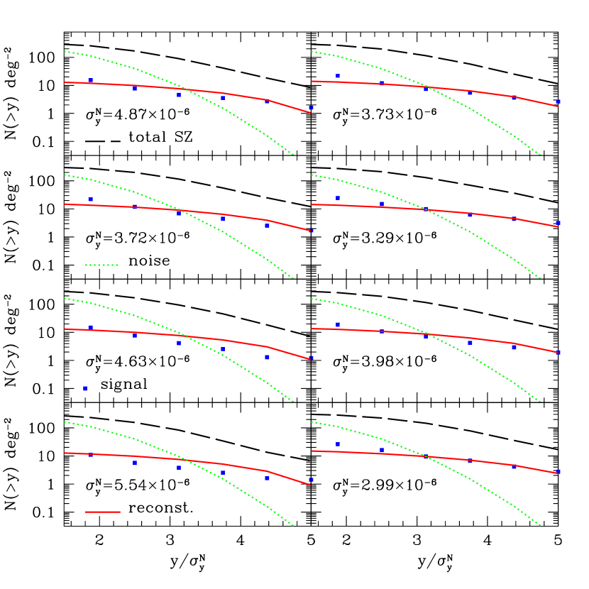
Figure 3: The number counts of local peaks per degree square as a cumulative function of the rescaled Comptonization parameter in each realization. The long-dashed, the dotted, and the solid lines correspond to the number counts of the total peaks of the SZE maps, the noise, and the reconstructed signals, respectively, while the square dots correspond to the number counts of the true signals from the original SZE map from simulations before the combination with the noise field.

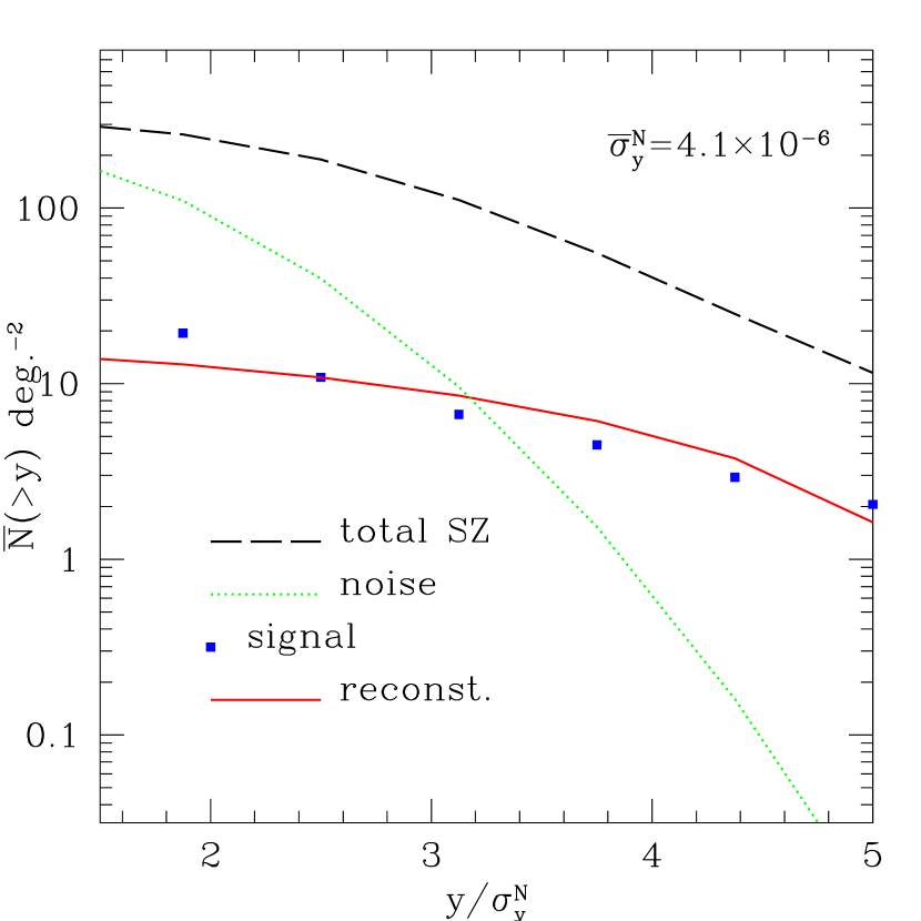
Figure 4: Same as Figure 3 but the averaged over the 8 realizations.

References

- Bahcall & Fan (1998) Bahcall, N., & Fan, X. 1998, ApJ, 504, 1
- Barbosa et al. (1996) Barbosa, D. Bartlett, J. G., Blanchard, A., & Oukbir, J. 1996, A&A, 314, 13
- Bond & Efstathiou (1987) Bond, J. R., & Efstathious, G. 1987, MNRAS, 226, 655
- Borgani et al. (1999) Borgani, S., Rosati, P., Tozzi, P., & Colin, N. 1999, ApJ, 517, 40
- Diaferio et al. (2003) Diaferio, A., Nusser, A., Yoshida, N. & Sunyaev, R. A. 2003, MNRAS, 338, 433
- Fan & Chiueh (2001) Fan, Z., & Chiueh, T. 2001, ApJ, 550, 547
- Glenn et al. (1998) Glenn, J., Bock, J. J., Chattopadhyay, G., Edgington, S. F., Lange, A. E., et al. 1998, Proc. SPIE 3357, 326
- Grego et al. (2001) Grego, L., Carlstrom, J. E., Reese, E. D., Holder, G. P., Holzapfel, W. L., Joy, M. K., Mohr, J. J., & Patel, S. 2001, 552, 2
- Henry (1997) Henry, J. P. 1997, ApJ, 489, L1
- Jenkins et al. (2001) Jenkins, A., Frenk, C. S., White, S. D. M., Colberg, J. M., Cole, S., Evrard, A. E., Couchman, H. M. P., Yoshida, N., 2001,MNRAS, 321, 372
- Lee (2002) Lee, J. 2002, ApJ, 578, L27
- Longuet-Higgins (1957) Longuet-Higgins, M. S. 1957, Phil Trans Roy Soc London A, 249, 321
- Lo et al. (2000) Lo, K. H., Chiueh, T. H., Martin, R. N., Ng, K. W., Liang, H., Pen, U. L, & Ma, C. P. 2000, in IAU symposium, Vol. 201, E31
- Molnar et al. (2002) Molnar, S. M., Birkinshaw, M.,& Mushotzky, R. F. 2002, ApJ, 570, 1
- Pen et al. (2002) Pen, U. L., Ng, K. W., Kesteven, M. J., & Sault, B. 2002, preprint (http://www.cita.utoronto.ca/ pen/download/Amiba/)
- Press et al. (1992) Press, W. H., Teukolsky, S. A., Vetterling, W. T., & Flannery, B. P. 1992, Numerical Recipes in Fortran (Univ. of Cambridge: New York)
- Sunyaev & Zel’dovich (1972) Sunyaev, R. A., & Zel’dovich, Y. B. 1972, Comm. Astrophys. Sp. Phys., 4, 173
- Viana & Liddle (1999) Viana, P. T. P., & Liddle, A. R. 1999, MNRAS, 303, 535
- Yoshida et al. (2001) Yoshida, N., Sheth, R. K. & Diaferio, A. 2001, MNRAS, 328, 669
- Yoshida (2002) Yoshida, N., 2002, PhD thesis, Ludwig-Maximilians-Univ., Munich
- Zhang et al. (2002) Zhang, P., Pen, U.L., & Wang, B. 2002, ApJ, 577, 555