Date: On the Steady Nature of Line-Driven Disk Winds

Abstract

We perform an analytic investigation of the stability of line-driven disk winds, independent of hydrodynamic simulations. Our motive is to determine whether or not line-driven disk winds can account for the wide/broad UV resonance absorption lines seen in cataclysmic variables (CVs) and quasi-stellar objects (QSOs). In both CVs and QSOs observations generally indicate that the absorption arising in the outflowing winds has a steady velocity structure on time scales exceeding years (for CVs) and decades (for QSOs). However, published results from hydrodynamic simulations of line-driven disk winds are mixed, with some researchers claiming that the models are inherently unsteady, while other models produce steady winds. The analytic investigation presented here shows that if the accretion disk is steady, then the line-driven disk wind emanating from it can also be steady. In particular, we show that a gravitational force initially increasing along the wind streamline, which is characteristic of disk winds, does not imply an unsteady wind. The steady nature of line-driven disk winds is consistent with the 1D streamline disk-wind models of Murray and collaborators and the 2.5D time-dependent models of Pereyra and collaborators. This paper emphasizes the underlying physics behind the steady nature of line-driven disk winds using mathematically simple models that mimic the disk environment.

1 Introduction

Accretion disks are commonly believed to be present in both cataclysmic variables (CVs) and quasi-stellar objects and active galactic nuclei (QSOs/AGN). In both types of object blue-shifted absorption troughs in UV resonance lines are sometimes present. Therefore, a popular scenario put forth to explain them involves outflowing winds emanating from an accretion disk, with the winds giving rise to absorption troughs in the objects’ spectra when they are viewed along preferential sight-lines. However, while this scenario is well motivated, the driving mechanism for the winds is still debatable.

In CVs, the P-Cygni type line profiles are observed only at inclination angles close to the pole (i.e., at $\lesssim 65^{\circ}$, where $0^{\circ}$ corresponds to the disk rotation axis) when there are high inferred mass accretion rates (e.g., Warner, 1995). Given these requirements, the obvious source of the wind material is the disk itself. The terminal velocities of the blue-shifted absorption troughs lie in the range $3,000-5,000\;{\rm km\;s}^{-1}$, which is comparable to escape velocities in the inner disk regions surrounding the white dwarf.

In QSOs, broad absorption lines (BALs) from an outflowing wind are observed in $>10\%$ of QSOs (e.g., Hewitt & Foltz, 2003). Outflow velocities up to $20,000-30,000\;{\rm km\;s}^{-1}$ are common. However, it is not clear to what degree the detection of BALs is an orientation-angle effect (e.g., Elvis, 2000), as is the case for CVs, or if instead BAL QSOs are a distinct QSO type with some special intrinsic or evolutionary properties (e.g., Boroson, 2002). Nevertheless, if accretion disks power QSOs/AGN, some viewing angle effects are likely to be present. Turnshek (1984) cited evidence for and speculated that the outflowing BAL gas may result from material being radially driven off an inner rotating disk, however the 1D model of Murray et al. (1995) was the first serious attempt to explain QSO/AGN observations using an accretion disk wind.

Another property that CVs and QSOs have in common is the existence of persistent velocity structure in their absorption troughs (when present) over significantly long time scales. This steady velocity structure, with changes $<10$ ${\rm km\;s}^{-1}$, persists at least up to years and decades, for CVs and QSOs, respectively. However, changes in the depths of the absorption have been observed in both classes of objects. For some relevant observations showing the behaviors see Froning et al. (2001) and Hartley et al. (2002) for results on CVs and Foltz et al. (1987) and Barlow et al. (1992) for results on QSOs. The behavior of the absorption in Q1303+308 (Foltz et al., 1987) is possibly very illustrative, with more recent data showing that the absorption depth has steadily increased over 20 years while the underlying velocity structure persists (Foltz, private communication).

To explain CVs Pereyra (1997) developed 2.5D dynamical models of line-driven disk winds (see also Pereyra, 1997; Pereyra, Kallman, & Blondin, 1997, 2000; Pereyra & Kallman, 2003). They concluded that steady wind solutions do exist and that wind terminal velocities are approximately independent of disk luminosity, similar to line-driven winds in early-type stars. They found that the mass-loss rate increased with disk luminosity and that rotational forces were important, causing velocity streamlines to collide and reduce speed, giving rise to an enhanced density region where the strongest absorption occurs. Although the approximations of single scattering and constant ionization were made, these models are generally consistent with observations and they show a strong dependence on inclination angle.

Proga, Stone, & Drew (1998) also developed 2.5D models for CVs (see also Proga, Stone, & Drew, 1999; Proga et al., 2002). Some of their results, for example the magnitude of the wind velocities, were similar to those obtained by Pereyra (1997). However, a significant difference between the two groups was that Proga, Stone, & Drew (1998, 1999) found unsteady flows characterized by large amplitude fluctuations in velocity and density on very short time scales.

For QSOs/AGN the 1D models of Murray et al. (1995) indicate that, with an appropriate x-ray shielding mechanism, a suitable accretion disk wind can be driven off by line radiation pressure. Unlike the case for CVs, the wind streamlines are approximately parallel to the disk at high velocities (i.e., close to inclination angles near $90^{\circ}$). The models of Murray et al. (1995) are able to account for the observed outflow velocities seen in BAL QSOs, the presence of detached absorption troughs seen in some BAL QSOs, and the approximate fraction of QSOs observed to have BALs. But the 2.5D QSO/AGN line-driven wind models of Proga, Stone, & Kallman (2000) challenge this result. Similar to their earlier CV disk-wind models, Proga, Stone, & Kallman (2000) and Proga et al. (2002) report finding intrinsically unsteady winds.

Proga and collaborators have suggested that since their unsteady line-driven disk-wind models are inconsistent with observational results, “that a factor other than line-driving is much more likely to be decisive in powering these outflows” (Hartley et al., 2002) and that “indeed radiation pressure alone does not suffice to drive the observed hypersonic flow” (Proga, 2003). However, the line-driven disk-wind models of Pereyra and collaborators (see Hillier et al., 2002) continue to find steady wind solutions, similar to the earlier CV models of Pereyra (1997) and Pereyra, Kallman, & Blondin (2000).

Thus, an impasse of sorts has developed with regard to the applicability of line-driven accretion disk wind models to CVs and QSOs/AGN. Clearly the observations indicate that steady winds do exist in these objects. However, while one group believes that steady line-driven winds can be achieved, the other group has advocated either abandoning this approach or adopting one that incorporates additional physics (e.g., magnetic fields) into the problem. Therefore, the objective of this work is to develop a series of semi-analytical models, independent of previous 2.5D dynamical efforts, to test for the existence/nonexistence of steady disk winds. We find that steady winds can exist and here we emphasize the physics behind these solutions by employing mathematically simple models designed to mimic a disk environment. In a subsequent paper we will present detailed numerical calculations.

In §2 we present the notation and general equations used in this paper. We define the nozzle function in §3 and discuss its relationship to steady wind solutions. In §4 we analyze the FSH02 model (Feldmeier, Shlosman, & Hamann, 2002). This analysis clearly demonstrates that an increase in gravity along a streamline, which is characteristic of disk winds, does not necessarily imply an unsteady wind. In §5 we present the standard simple models which demonstrate steady winds can exist. The summary and conclusions are presented in §6.

2 General Equations

2.1 Hydrodynamic Equations

Up to now our studies have indicated that for typical CV and QSO parameters temperature gradient terms do not produce significant changes in overall dynamical results. Thus, throughout this paper we assume that the wind is isothermal.

We use the Gayley ($\bar{Q}$,$\alpha$) line force parameterization (Gayley, 1995) for this study. This parameterization is used in place of the CAK $k$ parameter (Castor, Abbott, & Klein, 1975). The $\bar{Q}$ parameter has a direct physical interpretation (Gayley, 1995). The CAK $k$ and the Gayley $\bar{Q}$ parameters are related through

$$k={1\over 1-\alpha}\left(v_{th}\over c\right)^{\alpha}\bar{Q}^{1-\alpha}\;\;\;\;,$$ (1)

where $\alpha$ is the CAK line force parameter (Castor, Abbott, & Klein, 1975), $v_{th}$ is the ion thermal velocity, and $c$ is the speed of light.

The time-dependent hydrodynamic equations for a 1D system are (1) the mass conservation equation,

$$A{\partial\rho\over\partial t}+{\partial\over\partial z}(\rho VA)=0\;\;\;\;,$$ (2)

(2) the momentum equation,

$$\rho{\partial V\over\partial t}+\rho V{\partial V\over\partial z}=-\rho B+\rho{\kappa_{e}\over c}{\cal F}{\bar{Q}^{1-\alpha}\over 1-\alpha}\left({1\over\rho\kappa_{e}c}{\partial V\over\partial z}\right)^{\alpha}-{\partial P\over\partial z}\;\;\;\;,$$ (3)

and (3) the equation of state,

$$P=\rho\,b^{2}\;\;\;\;.$$ (4)

Here $z$ is the independent spatial coordinate which corresponds to the height above the disk (or the distance from the center of the star for stellar wind models), $t$ is the time, $V$ is the velocity, $A$ is the area which depends on $z$, $\rho$ is the density, $B$ represents the body forces which in this case is the gravitational plus continuum radiation force per mass, $\kappa_{e}$ is the Thomson cross section per mass, ${\cal F}$ is the radiation flux, $P$ is the pressure, and $b$ is the isothermal sound speed.

To simplify the momentum equation, we define the line opacity weighted flux $\gamma(z)$ as

$$\gamma(z)\equiv{\kappa_{e}\over c}{\cal F}(z){\bar{Q}^{1-\alpha}\over 1-\alpha}\left({1\over\kappa_{e}c}\right)^{\alpha}\;\;\;\;.$$ (5)

The time-dependent momentum equation can then be written as

$$\rho{\partial V\over\partial t}+\rho V{\partial V\over\partial z}=-\rho B+\rho\gamma\left({1\over\rho}{\partial V\over\partial z}\right)^{\alpha}-{\partial P\over\partial z}\;\;\;\;,$$ (6)

where the dependence of $\gamma$ on $z$ is implicit.

From equation (2) the stationary mass conservation equation is then

$$\rho\,VA=\dot{M}\;\;\;\;,$$ (7)

where $\dot{M}$ is the wind mass loss rate and the stationary momentum equation is

$$\rho V{dV\over dz}=-\rho B+\rho\gamma\left({1\over\rho}{dV\over dz}\right)^{\alpha}-{dP\over dz}\;\;\;\;.$$ (8)

2.2 Equation of Motion

Combining equations (4), (7) and (8), we find that the equation of motion is

$$\left(1-{b^{2}\over V^{2}}\right)V\,{dV\over dz}=-B+\gamma\left({A\over\dot{M}}V\,{dV\over dz}\right)^{\alpha}+{b^{2}\over A}{dA\over dz}\;\;\;\;,$$ (9)

and if we define

$$W\equiv{V^{2}\over 2}\;\;\;\;,$$ (10)

the equation of motion becomes

$$\left(1-{b^{2}\over 2W}\right){dW\over dz}=-B+\gamma\left({A\over\dot{M}}{dW\over dz}\right)^{\alpha}+{b^{2}\over A}{dA\over dz}\;\;\;\;.$$ (11)

2.3 Scaling of Physical Parameters

For each model, we define a value of $r_{0}$, $B_{0}$, $A_{0}$, and $\gamma_{0}$ as the characteristic distance, gravitational acceleration, area, and line-weighted opacity, respectively. The normalized spatial coordinate, $x$, body force, $g$, and area, $a$, are

$$x\equiv{z\over r_{0}}\hskip 24.0pt;\hskip 24.0ptg\equiv{B\over B_{0}}\hskip 24.0pt;\hskip 24.0pta\equiv{A\over A_{0}}\;\;\;\;.$$ (12)

The normalized line opacity weighted flux $f$ is

$$f\equiv{1\over\alpha^{\alpha}(1-\alpha)^{1-\alpha}}{\gamma\over\gamma_{0}}\;\;\;\;.$$ (13)

The characteristic value of the dependent variable $W$ is

$$W_{0}\equiv B_{0}r_{0}\;\;\;\;.$$ (14)

Then the characteristic velocity is given by

$$V_{0}\equiv\sqrt{2W_{0}}\;\;\;\;.$$ (15)

Based on the CAK stellar wind formalism (Castor, Abbott, & Klein, 1975), the characteristic wind mass loss rate is

$$\dot{M}_{CAK}\equiv\alpha(1-\alpha)^{1-\alpha\over\alpha}{A_{0}\gamma_{0}^{1\over\alpha}\over B_{0}^{1-\alpha\over\alpha}}\;\;\;\;.$$ (16)

The corresponding normalized variables are defined as

$$\omega\equiv{W\over W_{0}}\hskip 24.0pt;\hskip 24.0ptv\equiv{V\over V_{0}}\hskip 24.0pt;\hskip 24.0pt\dot{m}\equiv{\dot{M}\over\dot{M}_{CAK}}\;\;\;\;.$$ (17)

The normalized sound speed squared is

$$s\equiv{b^{2}\over 2W_{0}}\;\;\;\;.$$ (18)

Finally, by introducing the scaling relations from equations (12)-(18), the equation of motion becomes

$$\left(1-{s\over\omega}\right){d\omega\over dx}=-g+f\left({a\over\dot{m}}{d\omega\over dx}\right)^{\alpha}+{2s\over a}{da\over dx}\;\;\;\;.$$ (19)

This is the form of the equation of motion discussed throughout most of this paper. We emphasize at this point that for typical stellar, CV, and QSO parameters $s\ll 1$. For this reason $s$ has little influence on the fundamental characteristics of wind solutions, and thus will simply taken to be zero in much of the remaining analysis.

The question of the existence of a steady solution is then reduced to determining whether a value of $\dot{m}$ and a normalized function $\omega(x)$ exists such that it satisfies the boundary conditions and equation (19). A steady solution for a 1D hydrodynamical model exists if and only if equation (19) is integrable while simultaneously satisfying the boundary conditions. We note that once we show that steady solutions exist (§3), we then demonstrate their stability (§4 and §5) using numerical time-dependent hydrodynamical models based on the PPM numerical scheme (Colella & Woodward, 1984).

3 Nozzle Function and Critical Point

Motivated by analogies between line-driven winds and a supersonic nozzle (Abbott, 1980), we have found that insights can be obtained by defining and considering the nozzle function, $n(x)$. The relationship between the nozzle function, the critical point, and the existence/nonexistence of a steady 1D wind solution is elaborated in this section. Since mathematical expressions associated with critical point conditions have forms which readily allow for physical interpretation, we discuss the nozzle function and critical point conditions simultaneously.

In §3.1 we initially analyze the simple case where $s=0$ and $\alpha=1/2$. This case results in an explicit analytical expression for $d\omega/dx$ from the equation of motion [equation (19)]. In §3.2 we extend the results to include an arbitrary value for $\alpha$ ($0<\alpha<1$). In §A we briefly discuss the case of a finite sound speed ($s>0$). We note that although gas pressure does not produce significant corrections to wind mass loss rates and velocity laws for typical CV and QSO parameters, gas pressure effects do give rise to the necessity of a critical point in order for the wind solution to be steady. This result has been discussed in detail by Castor, Abbott, & Klein (1975) for the case of line-driven stellar winds. In §B we extend these arguments to the equation of motion presented here [equation(19)]. Finally, in order too illustrate the application of the nozzle function to line-driven winds, in §3.3 we apply it to the well-studied CAK stellar wind.

3.1 $s=0$ and $\alpha=1/2$

For this case the equation of motion becomes

$${d\omega\over dx}=-g+f\left({a\over\dot{m}}{d\omega\over dx}\right)^{1/2}\;\;\;\;,$$ (20)

and the question of the existence of a steady solution is reduced to the question of whether or not a value for $d\omega/dx$ can always be obtained when integrating the equation of motion.

From equation (20), one obtains

$${d\omega\over dx}={f^{2}a\over 4\dot{m}}\left[1\pm\sqrt{1-{4\dot{m}g\over f^{2}a}}\;\right]^{2}\;\;\;\;.$$ (21)

The nozzle function is defined to be

$$n(x)\equiv{f^{2}(x)a(x)\over 4g(x)}\hbox{\hskip 48.0pt}\left[={(fa)^{2}\over 4(ga)}\right]\hbox{\hskip 48.0pt}\;\;\;\;.$$ (22)

The expression for $d\omega/dx$ can now be written as

$${d\omega\over dx}={n(x)g(x)\over\dot{m}}\left[1\pm\sqrt{1-{\dot{m}\over n(x)}}\;\right]^{2}\;\;\;\;.$$ (23)

A steady solution must pass through a critical point, $x_{c}$, passing from a lower branch [corresponding to the “-” sign in equation (23)], to a higher branch [corresponding to the “+” sign in equation (23)] (see §B for details). Therefore, it must hold that

$$\dot{m}=\min[n(x)]\equiv n_{c}\equiv n(x_{c})\;\;\;\;,$$ (24)

where $n_{c}$ is the value of the nozzle function at the critical point.

Thus, one finds that the wind mass loss rate is determined by the minimum value of the nozzle function, where the wind mass loss rate is the maximum possible value that permits integration of the equation of motion (i.e., the maximum steady wind mass loss rate that the system can physically support).

The velocity law is obtained by integrating through the lower branch of the equation of motion from the critical point down to the sonic point, $x_{s}$, and by integrating the equation of motion through the upper branch from the critical point out to infinity. The constants of integration are determined through the conditions of continuity of the velocity law and the condition that $w(x_{s})=0$.

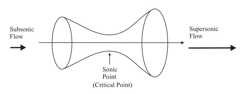
Figure 1: Supersonic Nozzle

Abbott (1980) discussed in detail the analogies between a stellar line-driven wind and a supersonic nozzle (a tube with a gas flow which starts subsonic and ends supersonic, see Figure 1). One similarity between a supersonic nozzle and the nozzle function of a 1D line-driven wind with negligible gas pressure is that a necessary condition for a steady flow is that the cross sectional area must have a minimum value within the nozzle (e.g., Landau & Lifshitz, 1997). Also, just as is the case with negligible gas pressure, the nozzle function in a line-driven wind must also present a minimum if a steady supersonic wind solution is to exist.

Another similarity, also discussed by Abbott (1980) for stellar winds, comes from the propagation velocity of density perturbations at the critical point. In a supersonic nozzle the sonic point, which is at the minimum of the nozzle cross sectional area, is the point where the flow velocity equals the propagation velocity of density perturbations (i.e., the sound speed). In a line-driven wind the critical point is the point where the flow velocity equals the backward velocity propagation of density perturbations, referred to as radiative-acoustic waves or Abbott waves (as opposed to sound waves). Due to the dependence of the line radiation force on the velocity gradient, density perturbations in a line-driven wind will travel at velocities different from sound speed. The propagation velocity will be subsonic in the forward direction (i.e., the direction of the line-driving force) and supersonic in the backward direction.

3.2 $s=0$ and $0<\alpha<1$

For this case the equation of motion becomes

$${d\omega\over dx}=-g+f\left({a\over\dot{m}}{d\omega\over dx}\right)^{\alpha}\;\;\;\;.$$ (25)

The question of the existence of a steady solution is again reduced to the question of whether or not a value for $d\omega/dx$ can always be obtained when integrating the equation of motion.

From an analysis similar to that presented by Castor, Abbott, & Klein (1975) for line-driven stellar winds, one finds that equation (25) has two solution branches which exist under the condition that

$$\dot{m}\leq\alpha(1-\alpha)^{1-\alpha\over\alpha}{f^{1\over\alpha}a\over g^{1-\alpha\over\alpha}}\;\;\;\;.$$ (26)

The two branches intersect at the critical point when both sides of equation (26) are equal.

This leads to the following definition of the nozzle function

$$n(x)\equiv\alpha(1-\alpha)^{1-\alpha\over\alpha}{f^{1\over\alpha}a\over g^{1-\alpha\over\alpha}}\;\hbox{\hskip 48.0pt}\left[=\alpha(1-\alpha)^{1-\alpha\over\alpha}{(fa)^{1\over\alpha}\over(ga)^{1-\alpha\over\alpha}}\;\right]\hbox{\hskip 48.0pt}\;\;\;\;\;.$$ (27)

The condition for the existence of the two solutions branches can now be written as

$$\dot{m}\leq n(x)\;\;\;\;.$$ (28)

Again we require a critical point type solution (see §B) and it follows that

$$\dot{m}=\min[n(x)]\equiv n_{c}\equiv n(x_{c})\;\;\;\;.$$ (29)

The wind mass loss rate and velocity law are determined just as in the $\alpha=1/2$ case.

3.3 CAK Model

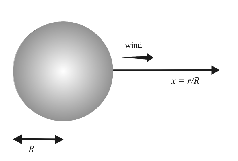
Figure 2: CAK Stellar Wind

Here we illustrate the concepts and notations which we have introduced by applying them to the well-known and well-studied CAK stellar wind (Castor, Abbott, & Klein, 1975). For simplicity we consider the case of zero sound speed only ($s=0$). For the CAK model (see Figure 2) we use the following characteristic scales

$$r_{0}=R\hskip 24.0pt;\hskip 24.0ptB_{0}={GM\over R^{2}}(1-\Gamma)\hskip 24.0pt;\hskip 24.0ptA_{0}=4\pi R^{2}\;\;\;\;;$$ (30)

and

$$\gamma_{0}={\kappa_{e}\over c}{{\cal L}\over 4\pi R^{2}}k\left(1\over\kappa_{e}v_{th}\right)^{\alpha}\;\;\;\;.$$ (31)

Here $R$ is the photospheric radius, $G$ is the gravitational constant, $M$ is the stellar mass, ${\cal L}$ is the stellar luminosity, and $\Gamma$ is the Eddington ratio given by

$$\Gamma={\kappa_{e}{\cal L}\over 4\pi GMc}\;\;\;\;.$$ (32)

For the CAK model the independent spatial variable is the distance, $r$, to the center of the star, and thus $x=r/R$.

With the corresponding substitutions, the equation of motion (for $s=0$) becomes

$${d\omega\over dx}=-{1\over x^{2}}+{1\over\alpha^{\alpha}(1-\alpha)^{1-\alpha}}{1\over x^{2}}\left({x^{2}\over\dot{m}}{d\omega\over dx}\right)^{\alpha}\;\;\;\;.$$ (33)

The expressions for the normalized variables for gravitational acceleration, line opacity weighted flux, and area are, respectively,

$$g={1\over x^{2}}\;\;\;\;;$$ (34)

$$f={1\over\alpha^{\alpha}(1-\alpha)^{1-\alpha}}{1\over x^{2}}\;\;\;\;;$$ (35)

and

$$a=x^{2}\;\;\;\;;$$ (36)

Substituting equations (34)-(36) into equation (27), we find

$$n(x)=1\;\;\;\;.$$ (37)

This constancy of the nozzle function implies that all spatial points become critical points (i.e., all points are a global minimum of the nozzle function). It follows that the normalized wind mass loss rate is given by:

$$\dot{m}=1\;\;\;\;.$$ (38)

The equation of motion becomes

$$\left(x^{2}{d\omega\over dx}\right)=-1+{1\over\alpha^{\alpha}(1-\alpha)^{1-\alpha}}\left(x^{2}{d\omega\over dx}\right)^{\alpha}\;\;\;\;,$$ (39)

which in turn implies

$$x^{2}{d\omega\over dx}={\alpha\over 1-\alpha}\;\;\;\;.$$ (40)

Integrating the last equation under the condition that $\omega(1)=0$ (zero velocity at photospheric height), we obtain the normalized velocity law

$$\omega={\alpha\over 1-\alpha}\left(1-{1\over x}\right)\;\;\;\;.$$ (41)

Expressing equations (38) and (41) in terms of the stellar parameters we obtain

$$\dot{M}={\alpha(1-\alpha)^{1-\alpha\over\alpha}\over(4\pi)^{1-\alpha\over\alpha}}{\left[{\kappa_{e}\over c}{\cal L}{\bar{Q}^{1-\alpha}\over 1-\alpha}\left(1\over\kappa_{e}c\right)^{\alpha}\right]^{1\over\alpha}\over[GM(1-\Gamma)]^{1-\alpha\over\alpha}}\;\;\;\;;$$ (42)

and

$$V=\left(\alpha\over 1-\alpha\right)^{1\over 2}\left(2GM(1-\Gamma)\over R\right)^{1\over 2}\left(1-{R\over r}\right)^{1\over 2}\;\;\;\;.$$ (43)

These are the well-known expressions derived by Castor, Abbott, & Klein (1975) for the wind mass loss rate $\dot{M}$ and the wind velocity law $V(r)$ in the asymptotic limit where $V$ is much greater than the sound speed.

4 FSH02 Model

Here we analyze the FSH02 model discussed by Feldmeier, Shlosman, & Hamann (2002). The motivation for studying the FSH02 in this work is twofold. First, the analysis clearly shows that an increase in gravity along a streamline, which is characteristic of disk winds, does not imply an unsteady wind. Second, for the case where $\alpha=1/2$, an explicit analytical solution can be found which will serve as a consistency check for the numerical codes.

The FSH02 model is defined through the following three equations

$$g(x)={x\over 1+x^{2}}\;\;\;\;;$$ (44)

$$a(x)=1\;\;\;\;;$$ (45)

and

$$f(x)=1\;\;\;\;,$$ (46)

where for these disk-like models $x$ is the distance along the vertical streamline normalized by the distance from the center of the disk. Assuming $s=0$ and $\alpha=1/2$, the equation of motion for the FSH02 model becomes

$${d\omega\over dx}=-{x\over 1+x^{2}}+\left({1\over\dot{m}}{d\omega\over dx}\right)^{1\over 2}\;\;\;\;.$$ (47)

From equation (22), the nozzle function for this model is given by

$$n(x)={1+x^{2}\over 4x}\;\;\;\;.$$ (48)

It follows that:

$$\min(n[x])={1\over 2}=n(1)\hbox{\hskip 48.0pt}(0\leq x)\;\;\;\;.$$ (49)

Therefore,

$$x_{c}=1\;\;\;\;\;\;\;\;{\rm and}\;\;\;\;\;\;\;\;\dot{m}={1\over 2}\;\;\;\;.$$ (50)

Substituting this value of $\dot{m}$ into equation (47) and integrating, with the additional condition that $\omega(0)=0$, we find

$$\omega(x)=x-1+\sqrt{1+x^{2}}-{\rm arcsinh}(x)-{1\over 2}\ln(1+x^{2})\;\;\;\;.$$ (51)

In Figure 3 we plot this velocity law in terms of $v\;=\sqrt{\omega}\;$.

Figure 4 shows the nozzle function $n(x)$ of the FSH02 model for $s=10^{-4}$ along with the product $\beta(\omega[x])\dot{m}$. These two graphs intersect at, and only at, the critical point. Since $\beta(\omega[x])$ is a monotonically increasing function, the critical point must be (slightly) to the right of the nozzle minimum. Also, since in the FSH02 model $da/dx=0$, it follows that for this model in particular the nozzle function is independent of $s$ [see equation (A2)].

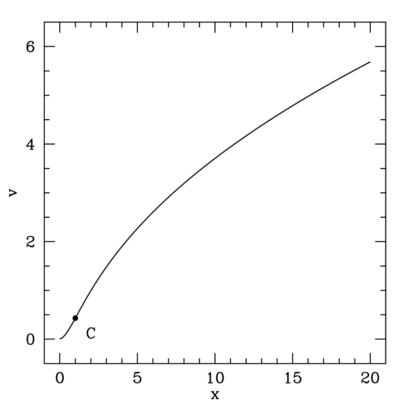
Figure 5: Velocity law for the FSH02 model ($s=10^{-4}$) obtained through numerical integration of the equation of motion. “C” denotes the critical point.

Figure 5 shows the velocity law of the FSH02 model for $s=10^{-4}$. One of the general results from the models we discuss in this paper is that gas pressure effects produce only minor corrections in the wind mass loss rate and in the velocity law; this is illustrated here by comparing Figures 3 and 5.

Figure 6 shows the results from the time-dependent simulation. The solid line is the initial velocity distribution at $t=0$; the short dash-long dashed line is the velocity distribution found once the code arrives at a steady state, which is in excellent agreement with the steady state solution found through the stationary codes. This figure shows that the steady solutions found through the stationary codes are stable.

Also, we wish to note here that care must be taken when numerically implementing the boundary conditions for the time-dependent simulations. As has been found for the case of line-driven stellar winds (Owocki, Cranmer, & Blondin, 1994; Cranmer & Owocki, 1996) and for the case of CV line-driven disk winds (Pereyra, Kallman, & Blondin, 2000; Pereyra & Kallman, 2003), by varying the numerical treatment of the boundary conditions, one may be lead to obtain unsteady flows which are numerical artifacts rather than intrinsic physical properties. A similar situation is found for the time-dependent simulations of MHD disk winds (rather than line-driven disk winds) (Ustyugova et al., 1999) in which nonstationary flow may be artifacts of initial conditions rather than being an intrinsic physical property of the flow. The numerical time-dependent hydrodynamical models are based on the PPM numerical scheme (Colella & Woodward, 1984).

A significant result from the analysis of the FSH02 model is that an increase in gravity along streamlines does not imply an unsteady wind, as is clearly shown in Figure 6.

5 The Standard “Simple” Models

As we discussed in the introduction, one of the aims of this work is to study simple models that illustrate the physics behind steady disk wind solutions without the elaborate mathematical calculations required by more realistic models. We proceed with this here.

The equation of motion for the standard models of this paper are given by equation (19). Each model is defined by specifying expressions for the normalized body force [$g(x)$; gravitational plus continuum radiation acceleration], the normalized area [$a(x)$], and the normalized line opacity weighted flux [$f(x)$].

The three standard models we consider have the same expressions for $g(x)$ and for $a(x)$, and differ only in the expression for $f(x)$. The $g(x)$ and $a(x)$ for the standard models are given by

$$g(x)={x\over(1+x^{2})^{3\over 2}}\;\;\;\;$$ (52)

and

$$a(x)=1+x^{2}\;\;\;\;.$$ (53)

Equation (52) is the exact expression for the vertical component of the gravitational field of a compact object at disk center, where $x=z/r_{0}$ and $r_{0}$ is the radius of the streamline at wind base. Equation (53) corresponds to the geometry of the 1D disk wind models of Pereyra, Kallman, & Blondin (1997). The motive for selecting this area function, in addition to it being a simple expression, is that it has the correct asymptotic behavior as $x\to 0$ (constant area: corresponding to parallel streamlines at the wind base) and as $x\to\infty$ ($a\sim x^{2}$: corresponding to the divergence of streamlines under spherical symmetry).

For simplicity, all standard models are assumed to have $\alpha=1/2$ .

5.1 The S Model

The standard “S” model is defined through the expression (Figure 7)

$$f(x)={1\over 1+x^{2}}\;\;\;\;.$$ (54)

The motive for selecting this expression for $f(x)$ is that it has the correct asymptotic behavior as $x\to 0$ (constant flux near the surface) and as $x\to\infty$ ($f\sim x^{-2}$).

In Figure 8 we present the nozzle function $n(x)$ of the S model (with $s=0$, neglecting gas pressure). For this model the nozzle function is a monotonically decreasing function with a finite value at infinity of $n_{\infty}=1/4$. The critical point is thus at infinity.

In Figure 9 we present the velocity law of the S model derived through numerical integration starting from the critical point. For the S model, when $s=0$, we assume that the critical point is at the highest spatial grid point ($x=20$ for the results presented here).

Now, as we have seen from a physical standpoint, the wind mass loss rate is determined by the minimum of the nozzle function. When neglecting gas pressure, the S model places the critical point at infinity. Thus, although a well defined stationary solution can mathematically be found, we are still left with the physical difficulty of having to account for the travel of information through an infinite distance (i.e., from the wind base to the critical point) in a finite time. However, once gas pressure effects are taken into account ($s>0$), the nozzle function has a well defined minimum at a finite distance from the wind base. In turn, the critical point is slightly to the right of the minimum, also at a finite distance from the wind base. Therefore, although the results indicate that gas pressure effects do not significantly affect the value of the wind mass loss rate or the wind velocity law, for the S model gas pressure is important in accounting for the existence of steady wind solutions, which we have confirmed through numerical time-dependent hydrodynamic codes. To show this in Figure 10, the nozzle function $n(x)$ is plotted simultaneously with the product $\beta([\omega(x)])\dot{m}$ of the S model for $s=10^{-4}$. Figure 11 shows the velocity law of the S model for $s=10^{-4}$. Our observation that gas pressure effects produce only minor corrections in the wind mass loss rate and the velocity law is illustrated by comparing Figures 9 and 11. Figure 12 shows the results from the time-dependent simulation for the S model. The solid line is the initial velocity distribution at $t=0$. The short dash-long dashed line is the velocity distribution found once the code arrives at a steady state, and this is in excellent agreement with the steady state solution found through the stationary codes. Since the time steady solution agrees with the stationary code, the stationary code solutions are stable.

5.2 The I Model

The “I” model is a modified version of the S model. The difference with respect to the S model is a subtle modification of the $f(x)$ function with the goal of mimicking the flux distribution of a standard Shakura-Sunyaev disk (Shakura & Sunyaev, 1973) in the inner disk region, where the scale height of the flux originating from the disk is slightly larger than the scale height of gravity for a compact mass at the center of the disk (e.g., Pereyra, 1997; Pereyra, Kallman, & Blondin, 2000).

The I model is defined through the expression (see Figure 13)

$$f(x)={1\over 1+\left(x\over 2\right)^{2}}\;\;\;\;.$$ (55)

In Figure 14 we present the nozzle function $n(x)$ of the I model (with $s=0$). The critical point is determined by the minimum of $n(x)$. In Figure 15 we present the velocity law of the I model derived through numerical integration starting from the critical point. We have also computed the nozzle function and the velocity law of the I model for $s=10^{-4}$, but the corresponding corrections due to gas pressure are not significant, so we do not show the plots here to avoid redundancy. Figure 16 shows the nozzle function $n(x)$ plotted simultaneously with the product $\beta([\omega(x)])\dot{m}$ for $s=10^{-4}$. These two graphs intersect at, and only at, the critical point. Figure 17 shows the results from the time-dependent simulation for the I model. The solid line is the initial velocity distribution at $t=0$; the short dash-long dashed line is the velocity distribution found once the code arrives at a steady state. Again we see that the time-dependent code converges and the results are in excellent agreement with the steady state solution found through stationary codes. Thus, this shows that the steady solutions found through stationary codes are stable.

5.3 The O Model

As with the I model, the “O” model is a modified version of the S model. The difference between the O model and the S model is a subtle modification of the $f(x)$ function, but now with the goal of mimicking the flux distribution of a standard disk in the outer region of the disk. In the outer region of a standard disk (Shakura & Sunyaev, 1973) the flux initially increases with height from the disk surface (e.g., Pereyra, 1997; Pereyra, Kallman, & Blondin, 2000). This increase is due to flux emanating from interior radii.

The O model is defined through the expression (see Figure 18)

$$f(x)={1+{x\over 1+x}\over 1+x^{2}}\;\;\;\;.$$ (56)

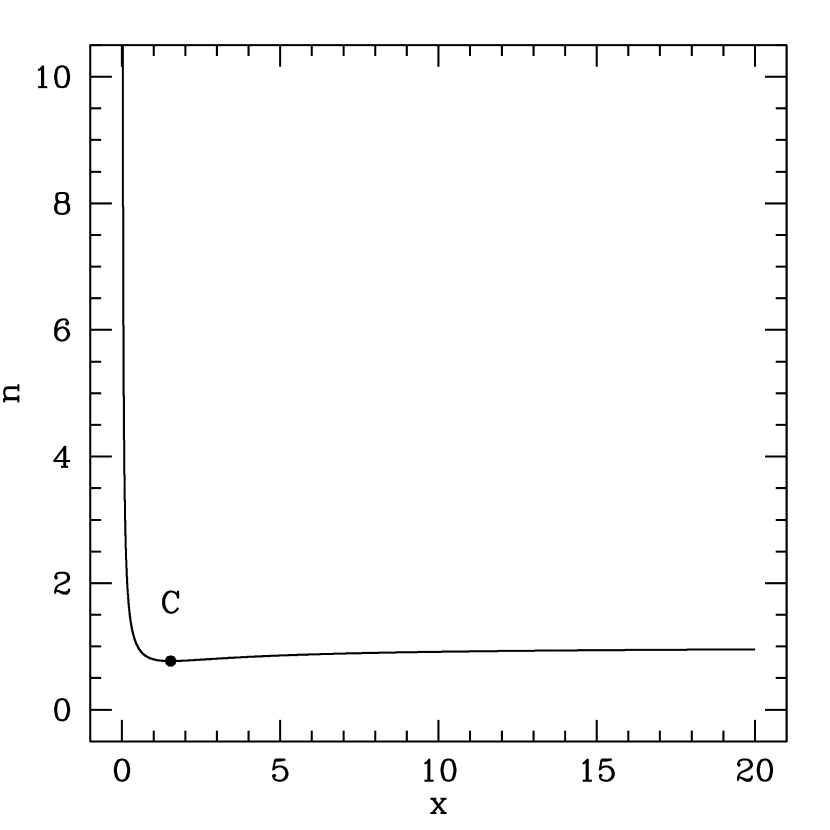
Figure 19: Nozzle function for the O model ($s=0$). When $s=0$ the critical point is determined by the position of the minimum of the nozzle function. “C” denotes the critical point.

In Figure 19 we present the nozzle function $n(x)$ of the O model (with $s=0$). The critical point is determined by the minimum of $n(x)$, which in turn gives the value of the normalized wind mass loss rate $\dot{m}$. In Figure 20 we present the velocity law of the O model derived through numerical integration starting from the critical point. As with the I model, we compute the nozzle function and the velocity law of the O model for $s=10^{-4}$, but the corresponding corrections due to gas pressure were insignificant, so again we do not plot this to avoid redundancy. Figure 21 shows the nozzle function $n(x)$ plotted simultaneously with the product $\beta([\omega(x)])\dot{m}$. These two graphs intersect at, and only at, the critical point. Since $\beta(\omega[x])$ is a monotonically increasing function, the critical point must be (slightly) to right of the nozzle minimum. Figure 22 shows the results from the time-dependent simulation for the O model. Again the solid line is the initial velocity distribution at $t=0$ and the short dash-long dashed line is the velocity distribution found once the code arrives at a steady state. Again this is in excellent agreement with the steady state solution found through the stationary codes, indicating that the steady solutions found through the stationary codes for model O are stable.

6 Summary and Conclusions

The objective of this work is to determine, in a manner independent of from results of previous numerically-intensive 2.5D hydrodynamic simulations, whether steady line-driven disk wind solutions exist or not. The motive behind this objective is to, in turn, determine whether line-driven disk winds could potentially account for the wide/broad UV resonance absorption lines seen in CVs and QSOs. In both types of objects, it is observationally inferred that the associated absorption troughs have steady velocity structure.

Our main conclusion is that if the accretion disk is steady, then the corresponding line-driven disk winds emanating from it can also be steady. We have confirmed this conclusion with more realistic (and mathematically more elaborate) models that we will present in a subsequent paper which implements the exact flux distribution above a standard Shakura-Sunyaev disk. This paper, in particular, has sought to emphasize on the underlying physics behind the steady nature of line-driven disk winds through mathematically simple models that mimic the disk environment.

The local disk wind mass loss rates and local disk wind velocity laws represented by the standard simple models of this work are a consequence of balancing the gravitational forces and the radiation pressure forces. Although gas pressure is present, we find that in our models inclusion of gas pressure gives rise to only minor corrections to the overall results.

The balance between gravitational and radiation pressure forces is represented quantitatively through a nozzle function. The spatial dependence of the nozzle function is a key issue in determining the steady/unsteady nature of supersonic wind solutions. In the case of a steady solution which neglects gas pressure effects, the minimum of the nozzle function determines the corresponding wind mass loss rate and the position of the minimum determines the critical point.

In the vicinity of the disk, gas pressure effects only produce minor corrections to the nozzle function, namely the critical point is shifted slightly to the right of the nozzle minimum, where the nozzle function has a positive derivative. However, in cases where the nozzle function is monotonically decreasing (as in the S model), these minor corrections generate a minimum in the nozzle function at a finite distance from the disk surface, i.e., shifting the critical point from infinity to a finite distance.

The steady nature of line-driven disk winds found in this paper is consistent with the steady nature of the streamline disk wind models of Murray and collaborators (Murray et al., 1995; Murray & Chiang, 1996; Chiang & Murray, 1996; Murray & Chiang, 1998), and it is also consistent with the 2.5D time-dependent models of Pereyra and collaborators (Pereyra, 1997; Pereyra, Kallman, & Blondin, 2000; Hillier et al., 2002; Pereyra & Kallman, 2003).

Appendix A Nozzle Function and Critical Point for $s>0$ and $0<\alpha<1$

For this case equation (19) is the equation of motion. From an analysis similar to that presented by Castor, Abbott, & Klein (1975), this equation, in the supersonic wind region, has two solution branches which exist under the condition that

$$\left(1-{s\over w}\right)\dot{m}\leq\alpha(1-\alpha)^{1-\alpha\over\alpha}{(fa)^{1\over\alpha}\over(ga-2s{da\over dx})^{1-\alpha\over\alpha}}\;\;\;\;.$$ (A1)

The two branches intersect at the critical point when both sides of equation (A1) are equal. As is apparent from equation (A1), the critical point conditions now depend on $x$ and $\omega$ rather than only $x$ as in cases where $s=0$ (see §3.1 and §3.2).

The definition of the nozzle function [cf. equation (27)] is now extended to include gas pressure in an isothermal wind using the following equation

$$n(x)\equiv\alpha(1-\alpha)^{1-\alpha\over\alpha}{(fa)^{1\over\alpha}\over(ga-2s{da\over dx})^{1-\alpha\over\alpha}}\;.$$ (A2)

We also define the function $\beta(\omega)$ as

$$\beta(\omega)\equiv 1-{s\over w}\;\;\;\;.$$ (A3)

The reason for choosing equation (A2) as the definition for the nozzle function when gas pressure effects are included are threefold. First, the definition of $\beta(\omega)$ [equation (A3)] allows for a simple relationship with the wind mass loss rate, conserving its physical interpretation respect to the $s=0$ case. As we discuss below, adding gas pressure effects will shift the critical point slightly to the right of the minimum where the nozzle function has a positive derivative. Second, equation (A2) reduces to the exact expression for the nozzle function for the $s=0$ case (equation [27]). Third, equation (A2) depends only on $x$ (not on $w$). The importance of the $x$-only-dependence is that it allows for the development of mathematical/numerical analysis of the problem without having to integrate the equation of motion. In particular, one could determine through the above nozzle function whether or not steady local wind solutions about a given spatial point exist, without having to integrate the equation of motion. This may lead to interesting future physical results, as well as serve as a testing tool for numerical models aimed at representing line-driven disk winds.

The condition for the existence of two solution branches can now be written as

$$\beta(\omega)\dot{m}\leq n(x)\;\;\;\;.$$ (A4)

If the condition that $\omega_{c}\gg s$ holds, then we find that

$$\dot{m}\approx n(x_{c})\;\;\;\;.$$ (A5)

Since we require a critical point type solution (see §B), a necessary condition for the critical point position is

$$\left.{dn\over dx}\right|_{x_{c}}>0\;\;\;\;.$$ (A6)

We will demonstrate this in more detail in a future paper. We emphasize that this applies when gas pressure effects are included in an isothermal wind. The actual critical point position is determined by a numerical iterative process that successively integrates the equation of motion until the condition $\omega(x_{s})=s$ is met. This is equivalent to the iterative process used by Castor, Abbott, & Klein (1975) in their original line-driven stellar wind paper. A consequence of equation (A6) is that when gas pressure effects are included, the critical point is no longer exactly at nozzle minimum, but in all the models we have explored, the critical point position is shifted slightly to the right of the nozzle minimum where the nozzle has a positive derivative.

Appendix B Necessity of a Critical Point for Steady Wind Solutions

As discussed above, the equation of motion [equation (19)] is integrable if upon integration one can always determine (i.e., a steady solution exists; assuming the boundary condition can be met),

$${d\omega\over dx}={d\omega\over dx}(x,\omega)\;\;\;\;.$$ (B1)

Assuming the boundary condition can be met, this means that a steady solution exists.

Viewing $dw/dx$ as a function of variables $x$ and $\omega$ which satisfies equation (19), one can divide the $x$-$w$ plane into five regions depending on whether a solution for $d\omega/dx$ exists. We do this below in a manner equivalent to, and following the notation of, Castor, Abbott, & Klein (1975) for early type stars:

$$\hbox{Region~{}I:}\;\omega<s\;\;{\rm and}\;\;-ga+2s{da\over dx}<0\;\hbox{: one solution};$$

$$\hbox{Region~{}II:}\;\omega>s\;\;{\rm and}\;\;-ga+2s{da\over dx}<0\;\;{\rm and}\;\;\beta(\omega)\dot{m}<n(x)\;\hbox{: two solutions};$$

$$\hbox{Region~{}III:}\;\omega>s\;\;{\rm and}\;\;-ga+2s{da\over dx}>0\;\hbox{: one solution};$$ (B2)

$$\hbox{Region~{}IV:}\;\omega>s\;\;{\rm and}\;\;-ga+2s{da\over dx}<0\;\;{\rm and}\;\;\beta(\omega)\dot{m}>n(x)\;\hbox{: no solution};$$

$$\hbox{Region~{}V:}\;\omega<s\;\;{\rm and}\;\;-ga+2s{da\over dx}>0\;\;\hbox{: no solution}.$$

We now make the following five assumptions with respect to the solution $\omega(x)$:

(1) $\omega(x)$ increases monotonically (i.e., $d\omega/dx>0$ [$dv/dx>0$] throughout the wind);

(2) the wind starts subsonic (i.e., the wind in the leftmost boundary is subsonic);

(3) the wind ends supersonic (i.e., the wind in the rightmost boundary is supersonic);

(4) the wind extends toward infinity (i.e., the rightmost boundary is infinity); and

(5) $d\omega/dx$ is continuous (i.e., continuous velocity gradients).

A wind solution must therefore start in Region I, since this is the only subsonic region which determines a value for $d\omega/dx$. Since we are assuming that the wind must end supersonic, the solution must continue on to Region II. Region II has two values for $d\omega/dx$, the lower/higher value corresponding to the lower/higher branch. The solution in Region I is continuous with the lower branch of Region II, therefore the needed solution must go from Region I to the lower branch of Region II as it goes from subsonic to supersonic.

Since the solution must extend toward infinity, and assuming that asymptotically

$$x\to\infty:\cases{a(x)\to x^{2}\cr g(x)a(x)\to{\rm const}}\;\;\;\;,$$ (B3)

it follows that

$$x\to\infty:-ga+2s{da\over dx}\to 4xs\;\;\;\;.$$ (B4)

Thus, toward infinity $-ga+2s(da/dx)>0$. This implies that the solution must end in Region III.

In turn, the solution of Region III is continuous with the upper branch of Region II. Therefore, at some large $x$, the solution must go from the upper branch of Region II into Region III. Continuity of $d\omega/dx$ implies that the lower and higher branch solutions must intersect at a point which is on the boundary between Region II and Region IV. This intersection point is the critical point of the solution.

For a wind that starts subsonic, reaches supersonic speeds, and extends to infinity, a solution to the 1D equations must then have the following sequence in $x-\omega$ plane as $x$ increases:

$\displaystyle\hbox{Region~{}I: subsonic,}\;-ga+2s{da\over dx}<0;$ $\displaystyle\hbox{Region~{}II: supersonic,}\;-ga+2s{da\over dx}<0\;\hbox{, lower branch,}\;\beta(\omega)\dot{m}<n(x);$ (B5) $\displaystyle\hbox{Region~{}II/Region~{}IV boundary: supersonic,}\;-ga+2s{da\over dx}<0,\;\hbox{\it critical point,}\;\beta(\omega)\dot{m}=n(x);$ $\displaystyle\hbox{Region~{}II: supersonic,}\;-ga+2s{da\over dx}<0,\;\hbox{upper branch,}\;\beta(\omega)\dot{m}<n(x);$ $\displaystyle\hbox{Region~{}III: supersonic,}\;-ga+2s{da\over dx}>0\ .$

We refer to solutions to the equation of motion with the above characteristics as critical point type solutions. We have therefore shown that a steady monotonically increasing continuous wind solution that starts subsonic, reaches supersonic speeds, and extends to infinity must be a critical point type solution of the equation of motion.

Figure 3: Analytic velocity law for the FSH02 model ($s=0$).

Figure 4: Nozzle function $n(x)$ and the product $\beta(\omega[x])\dot{m}$ for the FSH02 model ($s=10^{-4}$). “C” denotes the critical point.

Figure 6: Time dependent velocity distribution for the FSH02 model ($s=10^{-4}$). This plots shows that the steady solutions obtained through the stationary numerical codes are stable. In chronological order the plots are: solid line, dotted line, short dashed line, long dashed line, short dot-dashed line, long dot-dashed line, and short dash-long dashed line.

Figure 7: Line opacity weighted flux $f$ for the S model. The analytical form of the $f$ function for this model (equation [54]) was selected because (in addition to its simplicity) it has the correct asymptotic behavior as $x\to 0$ (constant flux near the disk surface) and as $x\to\infty$ ($f\sim x^{-2}$).

Figure 8: Nozzle function for the S model ($s=0$). Note that the nozzle function is monotonically decreasing throughout the spatial grid. For this model (with $s=0$) the nozzle function decreases monotonically to infinity, with a finite values at “infinity” of $n_{\infty}=1/4$.

Figure 9: Velocity law for the S model ($s=0$) obtained through numerical integration of the equation of motion. In the integration the critical point is assumed to be at the highest grid spatial point ($x=20$).

Figure 10: Logarithm of the nozzle function $\log(n[x])$ and the logarithm of the product $\log(\beta[\omega[x]]\dot{m})$ for the S model ($s=10^{-4}$). Both plots intersect at, and only at, the critical point. Note that (cf. Figure 8) when gas pressure effects are included ($s>0$) the nozzle function has a minimum at a finite distance (rather than having a minimum at infinity; cf. Figure 8). The critical point is denoted by “C”.

Figure 11: Velocity law for the S model ($s=10^{-4}$) obtained through numerical integration of the equation of motion. “C” denotes the critical point.

Figure 12: Time dependent velocity distribution for the S model ($s=10^{-4}$). This plots shows that the steady solutions obtained through the stationary numerical codes are stable. In chronological order the plots are: solid line, dotted line, short dashed line, long dashed line, short dot-dashed line, long dot-dashed line, and short dash-long dashed line. The code arrives at a steady state after a small multiple of the “crossing time” (the time it would take a particle in the wind to travel from the the disk surface [$x=0$] to the right end of the spatial grid [$x=20$] once the steady state is achieved).

Figure 13: Line opacity weighted flux $f$ for the I model. The analytical form of the $f$ function for this model (equation [55]) was obtained by adding a subtle change to the $f$ function of the S model (equation [54]) so as to produce an increase in the “scale height” of the flux. In turn, the motive for this is to mimic the inner disk region of a standard Shakura-Sunyaev disk where the scale height of the flux is slightly higher than the scale height of gravity for a compact object at disk center (cf. Figure 7).

Figure 14: Nozzle function for the I model ($s=0$). When $s=0$ the critical point is determined by the position of the minimum of the nozzle function. “C” denotes the critical point.

Figure 15: Velocity law for the I model ($s=0$) obtained through numerical integration of the equation of motion. “C” denotes the critical point.

Figure 16: Nozzle function $n(x)$ and the product $\beta(\omega[x])\dot{m}$ for the I model ($s=10^{-4}$). Note that when gas pressure effects are included ($s>0$), “$\beta(\omega[x])$” is a monotonically increasing function (equation [A3]); thus (since $\dot{m}$ is a constant) it follows that the critical point is shifted slight to the right of the nozzle minimum (rather than exactly at the nozzle minimum, as when $s=0$). “C” denotes the critical point.

Figure 17: Time dependent velocity distribution for the I model ($s=10^{-4}$). This plots shows that the steady solutions obtained through the stationary numerical codes are stable. In chronological order the plots are: solid line, dotted line, short dashed line, long dashed line, short dot-dashed line, long dot-dashed line, and short dash-long dashed line. The code arrives at a steady state after a small multiple of the “crossing time” (the time it would take a particle in the wind to travel from the the disk surface [$x=0$] to the right end of the spatial grid [$x=20$] once the steady state is achieved).

Figure 18: Line opacity weighted flux $f$ for the O model. The analytical form of the $f$ function for this model (equation [56]) was obtained by adding a subtle change to the $f$ function of the S model (equation [54]) so as to produce a flux distribution with an initially increasing flux from the disk surface and a subsequent local maximum. In turn, the motive for this is to mimic the outer disk region (rather than the inner disk region as in Figure 13), of a standard Shakura-Sunyaev disk, where the vertical radiation flux initially increases with height from the disk surface (cf. Figure 7).

Figure 20: Velocity law for the O model ($s=0$) obtained through numerical integration of the equation of motion. “C” denotes the critical point.

Figure 21: Nozzle function $n(x)$ and the product $\beta(\omega[x])\dot{m}$ for the O model ($s=10^{-4}$). Note that when gas pressure effects are included ($s>0$), “$\beta(\omega[x])$” is a monotonically increasing function (equation [A3]); thus (since $\dot{m}$ is a constant) it follows that the critical point is shifted slight to the right of the nozzle minimum (rather than exactly at the nozzle minimum, as when $s=0$). “C” denotes the critical point.

Figure 22: Time dependent velocity distribution for the O model ($s=10^{-4}$). This plots shows that the steady solutions obtained through the stationary numerical codes are stable. In chronological order the plots are: solid line, dotted line, short dashed line, long dashed line, short dot-dashed line, long dot-dashed line, and short dash-long dashed line. The code arrives at a steady state after a small multiple of the “crossing time” (the time it would take a particle in the wind to travel from the the disk surface [$x=0$] to the right end of the spatial grid [$x=20$] once the steady state is achieved).

References

- Abbott (1980) Abbott, D. C. 1980, ApJ, 242, 1183
- Barlow et al. (1992) Barlow, T. A., Junkkarinen, V. T., Burbidge, E. M., Weymann, R. J., Morris, S. L., Korista, K. T. 1992, ApJ, 397, 81
- Boroson (2002) Boroson, T. A. 2002, ApJ, 565, 78
- Castor, Abbott, & Klein (1975) Castor, J. I., Abbott, D. C., & Klein, R. I. 1975, ApJ, 195, 157
- Chiang & Murray (1996) Chiang, J., & Murray, N. 1996, ApJ, 466, 704
- Colella & Woodward (1984) Colella, P., & Woodward, P. 1984, J. Comput. Phys., 54, 174
- Cranmer & Owocki (1996) Cranmer, S., & Owocki, S. 1996, ApJ, 462, 469
- Elvis (2000) Elvis, M. 2000, ApJ, 545, 63
- Feldmeier, Shlosman, & Hamann (2002) Feldmeier, A., Shlosman, I., & Hamann, W.-R. 2002, ApJ, 566, 392
- Foltz et al. (1987) Foltz, C. B., Weymann, R. J., Morris, S. L., & Turnshek, D. A. 1987, ApJ, 317, 450
- Froning et al. (2001) Froning, C., Long, K., Drew, J., Knigge, C., & Proga, D. 2001, ApJ, 562, 693
- Gayley (1995) Gayley, K. G. 1995, ApJ, 454, 410
- Hewitt & Foltz (2003) Hewitt, P. C., & Foltz, C. B. 2003, AJ, 125, 1784
- Hartley et al. (2002) Hartley, L. E., Drew, J. E., Long, K. S., Knigge, C., & Proga, D. 2002, MNRAS, 332, 127
- Hillier et al. (2002) Hillier, D. J., Pereyra, N. A., Turnshek, D. A., & Owocki, S. P. 2002, BAAS, 34, 648
- Landau & Lifshitz (1997) Landau, L. D., & Lifshitz, E. M. 1997, Fluid Mechanics (Oxford: Butterworth-Heimann)
- Murray et al. (1995) Murray, N., Chiang, J., Grossman, S. A., & Voit, G. M. 1995, ApJ, 451, 498
- Murray & Chiang (1996) Murray, N., & Chiang, J. 1996, Nature, 382, 789
- Murray & Chiang (1998) Murray, N., & Chiang, J. 1998, ApJ, 494, 125
- Owocki, Cranmer, & Blondin (1994) Owocki, S., Cranmer, S., & Blondin, J. 1994, ApJ, 424, 887
- Pereyra (1997) Pereyra, N. A. 1997, Ph.D. Thesis, University of Maryland at College Park
- Pereyra, Kallman, & Blondin (1997) Pereyra, N. A., Kallman, T. R., & Blondin, J. M. 1997, ApJ, 477, 368
- Pereyra, Kallman, & Blondin (2000) Pereyra, N. A., Kallman, T. R., & Blondin, J. M. 2000, ApJ, 532, 563
- Pereyra & Kallman (2003) Pereyra, N. A., & Kallman, T. R. 2003, 582, 984
- Proga, Stone, & Drew (1998) Proga, D., Stone, J. M., Drew, J. E. 1998, MNRAS, 295, 595
- Proga, Stone, & Drew (1999) Proga, D., Stone, J. M., Drew, J. E. 1999, MNRAS, 310, 476
- Proga, Stone, & Kallman (2000) Proga, D., Stone, J. M., & Kallman, T. R. 2000, ApJ, 543, 686
- Proga et al. (2002) Proga, D., Kallman, T. R., Drew, J. E., & Hartley, L. E. 2002, ApJ, 572, 382
- Proga (2003) Proga, D. 2003, ApJ, 585, 406
- Shakura & Sunyaev (1973) Shakura, N. I., & Sunyaev, R. A. 1973, A&A, 24, 337
- Turnshek (1984) Turnshek, D. A. 1984, ApJ, 278, L87
- Ustyugova et al. (1999) Ustyugova, G. V., Koldoba, A. V., Romanova, M. M., Chechetkin, V. M. & Lovelace, R. V. E. 1999, 516, 221
- Warner (1995) Warner, B. 1995, Cataclysmic Variable Stars, (Cambridge University Press)