Neutrinos as astrophysical probes

Flavio Cavanna^a, Maria Laura Costantini^a, Ornella Palamara^b, Francesco Vissani^b

^aUniversità dell’Aquila e INFN - Via Vetoio, I-67010 L’Aquila, Italia

^bINFN, Laboratori Nazionali del Gran Sasso - S.s. 17 bis, I-67010 Assergi (AQ), Italia

The aim of these notes is to provide a brief review of the topic of neutrino astronomy and in particular of neutrinos from core collapse supernovae. They are addressed to a curious reader, beginning to work in a multidisciplinary area that involves experimental neutrino physics, astrophysics, nuclear physics and particle physics phenomenology. After an introduction to the methods and goals of neutrinos astronomy, we focus on core collapse supernovae, as (one of) the most promising astrophysical source of neutrinos. The first part is organized almost as a tale, the last part is a bit more technical. We discuss the impact of flavor oscillations on the supernova neutrino signal (=the change of perspective due to recent achievements) and consider one specific example of signal in detail. This shows that effects of oscillations are important, but astrophysical uncertainties should be thought as an essential systematics for a correct interpretation of future experimental data. Three appendices corroborate the text with further details and some basics on flavor oscillations; but no attempt of a complete bibliographical survey is done (in practice, we selected a few references that we believe are useful for a ‘modern’ introduction to the subject and suggest the use of public databases for papers [1] and for experiments [2] to get a more complete information).

Keywords: Neutrinos, core collapse supernovae, flavor oscillations.
PACS numbers: 14.60.-z, 23.40.Bw, 26.50.+x, 95.85.Ry, 97.60.-s

1 Neutrino astronomy, methods and goals

1.1 Main neutrino features

Neutrinos (and anti-neutrinos) of electron-, muon- and tau-flavor, are stable, neutral particles. This makes them important astrophysical probes; they are expected to point in the direction of the astrophysical site of production, as in the more standard case of astronomy with photons. Here we have in mind the case of ‘point astrophysical sources’; but of course ‘diffuse sources’ are also of importance.

In normal conditions, neutrinos are invisible. However, they can sometime interact and carry away or deposit energy in terrestrial detectors. By contrast, photons are much more easily absorbed than neutrinos; they can be observed more easily, but for the same reason their propagation can be more easily affected. In certain cases, neutrinos will be the most important signal (think for instance to neutrinos from big-bang nucleosynthesis, from the sun, or from a core collapse supernova).

Some neutrino interactions are of special interest for the following discussion. First,

$$\nu_{e}+e\to\nu_{e}+e,\ \ \ \nu_{\mu}+e\to\nu_{\mu}+e\ \ \mbox{[CC and NC elastic scattering]}$$ (1)

In these reactions an $e$ at rest – say, from an atom – is hit by the neutrino and acquires kinetic energy. An important feature is that the hit $e$ maintains the direction of the neutrino when the $\nu$ energy $E_{\nu}\gg m_{e}$ (“directionality”). The cross-section is low, $\sigma_{\nu}\sim G_{F}^{2}m_{e}E_{\nu}$ ($G_{F}$ is the Fermi coupling).
The (lowest energy) neutrino reactions are those of absorption on nucleons and on nuclei:

$$\begin{array}[]{l}\bar{\nu}_{e}+p\to e^{+}+n,\ \ \ {\nu}_{e}+n\to e+p\\ \bar{\nu}_{e}+(A,Z)\to e^{+}+(A,Z\!-\!1),\ \ \ {\nu}_{e}+(A,Z)\to e+(A,Z\!+\!1)\end{array}$$ (2)

these reactions have usually a threshold, and are only slightly directional (more quantitative statements requires care to details, see e.g., App. A). NC cross-sections on nuclei can be as large as $\sigma_{\nu}\sim G_{F}^{2}A^{2}E_{\nu}^{2}$, when a nucleus composed by $A$ nucleons reacts as a whole (coherent scattering). At higher energies, the absorption cross sections on nuclei become $\sim G_{F}^{2}A~{}m_{p}E_{\nu}$ (incoherent scattering). In this case, the nucleus is broken and/or hadronic resonances are excited.

1.2 Concepts of neutrino telescopes

Let us describe some concepts of neutrino detector, to illustrate what people mean by a ‘neutrino telescope’. (Supernova neutrino detectors fall in the first concept, normally.)

$\star$ One can instrument a large volume, possibly vetoing for external particle and wait for a charged particle coming apparently from nowhere—in actuality, created by a neutrino interaction. (Better to be underground for low counting rates, like those related to natural neutrino radiation.) Active volume can be a scintillator, a Čerenkov radiator, a layered target, a ‘bubble chamber-like’ detector. This method works from sub-MeV to several GeV energies, because it is subject to the condition that the (main part of the) event is contained in the detector. The number of events scales as

$$N=\mbox{Number of targets}\times\sigma_{\nu}\times\Phi_{\nu}\times\mbox{Time}~{}~{}~{}~{}\mbox{ ($\Phi$ denotes generically a flux).}$$

In particular, the event rate scales as the volume of the detector.

$\star$ One can set a muon counter and timing system underground (or underwater or under-ice), for muons that originate from neutrinos – as those coming from below. Detectors are located underground to avoid cosmic ray muons. This is the oldest method and works since muons suffer of mild energy losses till $\sim 500$ GeV (that corresponds roughly to Range${}_{\mu}\sim 1$ km in water). It applies from energies around a GeV till several hundred TeV; then the earth becomes opaque even to neutrinos (see e.g., [3]). The number of events and the $\nu$-induced muon flux scale respectively as:

$$N=\mbox{Surface}\times\Phi_{\mu}\times\mbox{Time}~{}~{}~{}\mbox{ where }~{}~{}\Phi_{\mu}=\Phi_{\nu_{\mu}}\times\sigma_{\nu_{\mu}}\times N_{A}\times\mbox{Range}_{\mu}.$$

In particular, the signal scales as the area of the detector (actual target being the earth, the water or the ice where the detector is located).

$\star$ By an extension of previous concept, one could use the earth atmosphere as a target for high energy neutrinos to produce inclined air showers; or, use mountains to convert almost horizontal $\nu_{\tau}$ of very high energy into visible tau’s. In this way, we could observe neutrinos of highest energies. The search of inclined air showers is just a spin-off of extensive air shower arrays research activity. Till now, however, no positive detection has been claimed.

In principle we would like to measure a lot of quantities: a) direction of the charged lepton; b) its energy; c) its charge; d) tag the flavor; e) tag the time of arrival; f) check occurrence of secondaries ($n,\gamma,$ charged hadrons). In practice, one has to find a compromise between the various and contrasting needs of an experiment, e.g. between the wish to have a very ‘granular’ detector able to see all the details of the reaction and the need to monitor a big amount of matter.

1.3 Chances for neutrino astronomy

In short, the goal is to use neutrinos to probe astrophysical sources; the information from $\nu$ can be complementary to the one from $\gamma$. Some important possibilities in this connection are:

(1) Solar neutrinos [0.1-20 MeV] There is little doubt that this is ‘$\nu$-astronomy’. Among the results of a very successful program of observations pioneered by Homestake we quote: a) low energy $\nu$ experiments Gallex/GNO and SAGE prove that the pp-chain (initiated by $pp\to De^{+}\nu_{e}$) is the main energy source; b) the physics of the center of the sun ($\rho_{c}\sim 150$ g/cm³) is probed. There is consistency with the theory of solar oscillation eigen-modes (helioseismology). c) Neutrino oscillations of a type predicted in MSW theory are indicated. Future observations will aim at the Beryllium line (Borexino, KamLAND) and at real time pp-neutrino detection.
(2) Atmospheric neutrinos [0.05-1000 GeV] primary cosmic rays (CR) come isotropically on earth atmosphere and they are not completely understood; they are not thought as astronomy, but they belong to astrophysics as much as to particle physics. Atmospheric neutrinos give a very significant indication of oscillations, especially thanks to Super-Kamiokande results. The study of CR secondaries as the electromagnetic component, muons or atmospheric neutrinos, permits us to investigate CR spectra and their interactions with earth atmosphere (which is not that different from possible sites of production of CR). In the present context, atmospheric neutrinos will be thought just as an important background.
(3) Neutrinos from cosmic sources [unknown energies] This is a vast field and includes a large variety of approaches of observation and of objects; presumably, also unknown objects [4]. For instance, one can search for an excess of neutrino events over the expected background by selecting a solid angle–observation window–around a cosmic source (say, an active galactic nucleus) or an appropriate time window around a cosmic events (say, a gamma ray burst). Other possibilities are to search for self-trigger (excess of multiple ‘neutrino’ events), or coincidence with other neutrino- or with gravitational wave-detectors. The observation of point (or diffuse) sources is a very important goal: e.g., $\nu$ (and $\gamma$) astronomy above TeV can shed light on the problem of the origin of CR. Till know, several experiments like LSD, MACRO, LVD, Super-Kamiokande, Soudan2, Baksan, AMANDA, EAS-TOP, HiRES and other ones produced upper limits on the fluxes. In future, this type of search will be conducted by ANTARES, AUGER, ICECUBE. One of the main hopes is that the neutrino energy spectrum remains very hard till $\sim$100 TeV, as suggested by observed gamma spectra at 1-10 TeV (another one is that the prompt neutrino background–from charm–is not overwhelming.)
(4) Supernova neutrinos [few-100 MeV] (this ‘cosmic’ source is singled out, since it is the topic of the rest of the paper). As recalled in next section, most of core collapse supernova energy is carried off by neutrinos of all flavors. About 20 events were detected in 1987 by simultaneous observations of Kamiokande II, IMB, Baksan detectors [5] from such a supernova, SN1987A, located in the Large Magellanic Cloud, at a distance $D\approx 50$ kpc. Usually, all these events are attributed to inverse $\beta$-decay, the one with the largest cross-section (see App. A). The experimental detection of these events begun extragalactic neutrino astronomy. The agreement with the expectations is reasonable.
Many operating neutrino detectors like Super-Kamiokande, SNO, LVD, KamLAND, Baksan, AMANDA could be blessed by the next galactic supernova. Other detectors like ICARUS and Borexino will also be able to contribute to galactic supernovae monitoring in the future. This activity will have a big payoff in astro/physics currency: core collapse SN are a source of infrared, visible, $X$, and $\gamma$ radiation and possibly of gravitational waves; they are of key importance for origin of galactic CR, for reprocessing of elements, presumably for the dynamics of magnetic fields; they are likely to be related to cosmic phenomena like gamma ray bursts; etc. In the following, we focus only on supernova neutrinos.

1.4 Galactic, extragalactic and relic supernovae

We close this introduction by classifying and discussing the possible observations of SN neutrinos. (Note that, unless said otherwise, the term supernova means always core collapse supernova in these notes, even though this is an abuse of notation – supernovae of type Ia are very important in cosmology and astrophysics, and are not core collapse events).

The hope of existing neutrino telescopes is the explosion of a galactic supernova, for the simple fact that the $1/D^{2}$ scaling of the flux is severe. In water or scintillator detectors one expects roughly 300 $\bar{\nu}_{e}$-events/kton, for a distance $D$=10 kpc – when our galaxy has a radius of some 15 kpc and we are located at 8.5 kpc from its center. Various authors estimated the rate of occurrence of core collapse supernovae; for our galaxy, this ranges from $\sim 1/(10$ y) to $\sim 1/(100$ y). A recent study [6] of the correlations of $\sim 200$ observed supernovae at cosmological distances with the blue luminosity of their host galaxy yields 1/(50-100 y). A $\sim 1/(10$ y) lower limit can be already established, since existing $\nu$-telescopes did not observe any event yet. Often, one recalls the possibility that SN events can take place in optically obscured regions of our galaxy; however, one should also remind that, beside $\nu$’s, there are other manners to investigate the occurrence of such a phenomenon, e.g., from the released infrared radiation.

Curiously enough, galactic neutrino astronomy is still to begin, but as recalled extragalactic neutrino astronomy begun several years ago with SN1987A. In principle, one should profit of the wealth of galaxies around us (say, those in the ‘local group’) to get events at human-scale pace. In practice this is difficult, because core collapse SN takes place only in spiral or irregular galaxies and not in elliptical ones. The only other large spiral galaxy of the local group is Andromeda (M31) but (1) its mass is presumably half of our galaxy, (2) its distance is about 700 kpc. A half-a-megaton detector (as the one suggested as a followup of Super-Kamiokande to continue proton decay search) should get 30 events if efficiency is unit. Perhaps, the best chance would be another SN from Large Magellanic cloud (an irregular galaxy) but the odds for such an event are not high.

Another interesting possibility is the search for relic supernovae, namely the neutrino radiation emitted from past supernovae. The practical method is to select an energy window around $20-40$ MeV, where atmospheric or other neutrino background is small, searching for an accumulation of neutrino events there with more-or-less known distribution. The best limit has been obtained by the Super-Kamiokande water-Čerenkov experiment [7], and the sensitivity is approaching the one requested to probe interesting theoretical models. In principle, one can suppress the main background (muons produced below the Čerenkov threshold) by identifying the neutron from neutrino inverse $\beta$-decay reaction. This could be perhaps possible by loading the water with an appropriate nucleus with high n-capture rate, that should absorb the neutron and yield visible $\gamma$ eventually see e.g., [8].

2 Supernova neutrinos

In Sec.2.1 and 2.2 we present theoretical expectations on supernova neutrinos. More precisely, we describe the expected sequence of events of the ‘delayed scenario’. This is the current theoretical framework [9] [10], possibly leading to SN explosion. In Sec.2.3 we discuss generalities of SN neutrino oscillations. We provide the basic concepts and formulae and discuss the impact on the fluxes. (The basic terminology and results are recalled in App. C, but a real beginner could conveniently consult review articles or texts before reading this section. For a more advanced reading, we list in Ref. [14] some recent research works on oscillations of supernova neutrinos.) Finally, we complete the discussion and show an application of the formalism in Sec.2.4, by considering the reaction $\nu_{e}$ Ar$\to$K${}^{*}e^{-}$ as a signal of supernova neutrinos in an Argon based detector.

However, the reader should be warned: at present it turns out to be difficult (perhaps impossible) to simulate a SN explosion. This could be due to a very complex dynamics; or, it could indicate that some ingredient is missing (such as an essential role of rotation, of magnetic fields, etc); or that there is nothing like a ‘standard explosion’; or, worse, a combination of previous possibilities. In short, we have not a ‘standard SN model’ yet and this makes supernova neutrinos even more interesting.

2.1 Gravitational collapse and the ‘delayed scenario’

Usually, the life of a star is characterized by a quasi-equilibrium state between gravity and nuclear forces. However, the dramatic conclusion the brief-some million years-life of a very massive star of $\sim 10-40\ M_{\odot}$ is something very different, a core collapse supernova.

Stellar evolution forms an iron-core, inert to nuclear reactions. This is supported by degeneracy pressure of (quasi)free electrons, but when it exceeds the Chandrasekhar mass of $\sim 1.4M_{\odot}$ (radius $\sim 3\times 10^{3}$ km) it collapses under its weight. The neutron density of the innermost part of the core (the ‘inner-core’, $\sim 0.6M_{\odot}$) enlarges progressively due to iron photo-dissociation followed by electron capture – “infall” phase. When it reaches nuclear densities the increase in matter pressure is sufficient to halt the collapse. The ‘outer-core’ (which is still free-falling onto the center of the star) undergoes a bounce on the stiff inner-core. In this moment, an outward-going shock-wave forms, producing a prompt neutronization in the shocked material whose mass is about $\sim 0.4M_{\odot}$ – “flash” phase. Then, the shock wave enters a phase of stall, trying to make its way through the outer part of the core. This turns the propagating wave into an shock of accretion that involves rest of the initial iron core, $\sim 0.5M_{\odot}$ – “accretion” phase. During this phase, convective motions and neutrinos (the ‘delayed mechanism’) should revive the shock (that subsequently will eject outer star’s layers – the SN explosion). The inner core settles in a new quasi-equilibrium state called protoneutron star, that smoothly cools and contracts radiating neutrinos of all types – “cooling” phase. Eventually this leads to the formation of a neutron star (NS), occasionally seen as a pulsar. Its mass is $M_{\mathrm{ns}}=1-2\ M_{\odot}$, and its radius scales roughly as $R_{\mathrm{ns}}\approx 20\mbox{ km}\times(M_{\odot}/M_{\mathrm{ns}})^{1/3}$, due to degenerate character of the equation of state. The main features of the collapse process, subdivided in the various phases mentioned above, are summarized in Tab. 1.

Table 1: Schematic description of collapse and neutrino emission in the delayed scenario. (SN progenitor mass $M_{\star}\sim 13\pm 3M_{\odot}$). In the first four rows, the main phases are identified. Their conventional names are given in Column-1 and the expected dynamics is described in Column-2. Only the main reactions and $\nu$-processes (Column-3) are listed. The last row refers to the newborn n-star: when temperature decreases to $\sim 10^{9}$ K it becomes transparent to neutrinos; the emission continues for $\Delta t\sim 10^{5}$ yr, until the temperature drops to $\sim 10^{8}$ K.

Collapse Phase	Dynamics	$\nu$ Process	Duration	Energetics
“Infall”	Iron Core Collapse	$\nu_{e}$-emission	$\sim 100$ ms
(early neutronization)		$e^{-}+p\to n+\nu_{e}$
of inner core	$\gamma+Fe\to 13^{4}He+4n$		$\Delta t_{inf}\lesssim 25$ ms	$\delta_{inf}\leq 1$% ${\cal E}_{B}$
$\sim 0.6M_{\odot}$	${}^{4}He\to 2n+2p$	$\nu_{e}$-trapping
		$\nu_{e}+A\to\nu_{e}+A$
		$\nu_{e}+n\to p+e^{-}$
“Flash”	Bounce. Shock wave	$\nu_{e}$-burst	[$t\equiv t_{0}$]
(prompt neutronization)		$e^{-}+p\to n+\nu_{e}$		$\delta_{fl}\sim 1$% ${\cal E}_{B}$
of (part of ) outer core	$\gamma+Fe\to 13^{4}He+4n$	at $\nu_{e}$-sphere	$\Delta t_{fl}\lesssim 10$ ms
$\sim 0.4M_{\odot}$
“Accretion”	Stall of shock wave	$\bar{\nu}_{e}$-emission
Mantle neutronization		$e^{+}+n\to p+\bar{\nu}_{e}$
$\sim 0.5M_{\odot}$	$\gamma\to e^{+}e^{-}$
		$\nu_{i}$-emission
		$e^{+}e^{-}\to\nu_{i}\bar{\nu}_{i}$	$\Delta t_{accr}\lesssim 500$ ms	$\delta_{accr}\approx 10$ % ${\cal E}_{B}$
	Proto n-star formation
Delayed shock revival		$\nu$-heating
	SN explosion	$\nu_{e}+n\rightleftharpoons p+e^{-}$
		$\bar{\nu}_{e}+p\rightleftharpoons n+e^{+}$
“Cooling”	Mantle contraction	$\nu_{i}$-emission
residual neutronization	$\gamma\to e^{+}e^{-}$	$e^{+}e^{-}\to\nu_{i}\bar{\nu}_{i}$	$\Delta t_{cool}\sim 10$ s	$\delta_{cool}\sim 90$ % ${\cal E}_{B}$
		at $\nu_{i}$-sphere
n-star		$\nu$-‘fading’
$M_{\mathrm{ns}}\sim 1.4M_{\odot}$	Steady state	$n~{}n\to n~{}p~{}e^{-}\bar{\nu}_{e}$		few % ${\cal E}_{B}$
$R_{\mathrm{ns}}\simeq 18$ km		$n~{}p~{}e^{-}\to n~{}n~{}\nu_{e}$
$\rho\simeq 3\times 10^{14}$ g/cm3

The most important aspect to note is that the gravitational binding energy released during the collapse process (up to the n-star formation) is huge, about

$${\cal E}_{B}\simeq G_{N}\ \frac{3}{5}\frac{M^{2}_{\mathrm{ns}}}{R_{\mathrm{ns}}}\approx(1-5)\times 10^{53}\ \textrm{erg}$$ (3)

(3/5 is for a uniform density distribution) that is about $\sim 10\%$ of the n-star rest mass energy $M_{\mathrm{ns}}\,c^{2}$. This is much bigger than the kinetic energy of the ejecta $E_{\mathrm{kin}}\sim 10^{51}$ ergs $\approx 1\%$ ${\cal E}_{B}$ (a typical velocity of the shock wave is 4-5000 km/s, ejecta mass $M_{\mathrm{ej}}\sim 10M_{\odot}$). Also much bigger than what is needed to dissociate the outer iron core $0.6M_{\odot}/m_{n}\times(2.2\ \mathrm{MeV})=2\times 10^{51}$ erg since the mass of ⁵⁶Fe is 123 MeV smaller than $13m_{\alpha}+4m_{n}$ – but this could be optimistic and the energy losses suffered by the shock wave even larger. The energy that goes in photons is very small, $E_{\mathrm{lum}}\approx 10^{49}$ erg $\approx 0.01\%$ ${\cal E}_{B}$ (sufficient to outshine host galaxy though!) and the gravitational wave part is unknown (and depends on the detailed dynamics of the collapse) but it is probably even less. The overwhelming part of this huge energy is carried away by neutrinos (main reactions leading to $\nu$ production in the various collapse phases are reported in Tab. 1). The neutrino ‘luminosity’ can be roughly estimated noting that $\sim 10^{53}$ erg are emitted in a few seconds in the cooling timescale, and thus ${L}_{\nu}\approx 3\times 10^{19}\ {L}_{\odot}$: the supernova neutrino burst outshines the entire visible universe. (Incidentally, we feel there is something poetic in these quasi-spherical SN neutrino shells that propagate freely in the Universe).

2.2 Neutrino fluxes

Here, we describe in some detail the neutrino fluxes. First we discuss the general characteristics and present a phenomenological survey, and then we discuss how their luminosity, energy spectrum and possible non-thermal effects can be parameterized. We ought to recall the three relevant types of neutrino fluxes:

$\nu_{e},\ \ \bar{\nu}_{e}\ \mbox{ and }\ \nu_{x}$

where $x$ is anyone among muon and tau (anti)neutrinos. In fact, $\nu_{\mu}$ and $\bar{\nu}_{\mu}$ have similar properties, $\nu_{\mu}$ and $\nu_{\tau}$ are produced by neutral currents (NC) in the same manner and probably, muons are present only in the innermost core; thus $\nu_{\mu}$, $\bar{\nu}_{\mu}$, $\nu_{\tau}$ and $\bar{\nu}_{\tau}$ should have a very similar distribution.

Let us begin by describing the general properties of the neutrino fluxes. As seen in Sec.2.2, in the delayed scenario the collapse has four main phases. Correspondingly, we distinguish between an early neutrino emission, during the “infall” and “flash” phase and a late phase of emission (or ‘thermal phase’), during the “accretion” and “cooling”: see Tab. 1 for more details. The most uncertain phase is certainly the one of “accretion”, that, together with “cooling”, accounts for most of the energetics. Perhaps, one could argue that a fair estimate of errors should be just 100 %. In support of this (apparently too conservative) statement, we recall that we have not ab initio calculations of these fluxes and alternative (even if incomplete or still speculative) scenarios have been considered. Furthermore, the calculations that tried to estimate the effect of rotation (by Imshennik and collaborators and more recently by Fryer and Heger [11]) found very different fluxes and in particular a severe suppression of muon and tau neutrinos.

Reference ranges on neutrino energies averaged on time (starting at flash time, $t_{0}=t_{fl}$) found comparing a number of numerical calculations are:

$$\begin{split}\langle E_{\nu_{e}}\rangle=10-12\mbox{ MeV },\\ \langle E_{\bar{\nu}_{e}}\rangle=11-17\mbox{ MeV },\\ \langle E_{\nu_{x}}\rangle=15-25\mbox{ MeV },\end{split}$$ (4)

The reason of this hierarchy is that neutrinos that interact more – $\nu_{e}$ and $\bar{\nu}_{e}$ undergo CC reactions, beside NC – decouple in more external regions of the star at lower temperature. In other words, each neutrino type has its own ‘neutrino-sphere’ – $\nu_{e}$’s one being the outermost.
The approximate amount (average values over flash and accretion and cooling duration) of the total energy ${\cal E}_{B}$ carried away by the specific flavor is

$$\begin{split}{\cal E}_{\nu_{e}}=f_{\nu_{e}}\ {\cal E}_{B}~{}~{}~{}\mbox{with:}~{}~{}f_{\nu_{e}}=17-22\ \%\\ {\cal E}_{\bar{\nu}_{e}}=f_{\bar{\nu}_{e}}\ {\cal E}_{B}~{}~{}~{}\mbox{with:}~{}~{}f_{\bar{\nu}_{e}}=17-28\ \%\\ {\cal E}_{\nu_{x}}=f_{\nu_{x}}\ {\cal E}_{B}~{}~{}~{}\mbox{with:}~{}~{}f_{\nu_{x}}=16-12\ \%\end{split}$$ (5)

The approximate equality found in numerical calculations has been called ‘equipartition’, but in our understanding, there is no profound reason behind this result. We recall again that these numbers should be regarded with caution.

Next, we would like to introduce a general formalism to describe parameterized neutrino fluxes. Such a description requires (a) to know the distance of production $D$, (b)  to assume a distribution over the solid angle (usually this is isotropic, up to corrections of the order of $\sim 1-10$ % at most) (c) to assign a ‘luminosity’ function $d{\cal E}_{i}/dt$ (energy carried by neutrinos per unit time) for each neutrino species, (d) to describe the neutrino energy spectrum, presumably black-body of Fermi-Dirac type:

$$n(E;\eta_{i},T_{i})=\frac{1}{N}\frac{E^{2}}{[1+\exp(E/T_{i}-\eta_{i})]}~{}~{}~{}\mbox{ with the normalization factor}~{}~{}N=T^{3}_{i}F_{2}(\eta_{i})$$ (6)

where $T_{i}$ is the temperature expressed in energy units (the normalization factor $N$ and the meaning of $F_{2}$ are explained in App. B). Possible non-thermal effects are often described by introducing a parameter $\eta_{i}$ that modifies the shape of the distribution. This parameter is not a chemical potential (it is not subject to the condition $\eta_{\nu}=-\eta_{\bar{\nu}}$) and it is often called the pinching factor. (However, it is not excluded that the true non-thermal effects are even more dramatic and the high energy tail of the spectrum is cutoff as $e^{-(E/E_{0})^{2}}$, where $E_{0}$ is another new parameter).
At a distance $D$ from the source, the flux differential in energy and time ($t\geq t_{fl}$) is:

$$\frac{d^{2}\Phi^{0}_{i}}{dEdt}=\frac{1}{N^{\prime}}\frac{1}{4\pi D^{2}}\frac{d{\cal E}_{i}}{dt}~{}n(E;\eta_{i},T_{i})~{}~{}~{}\mbox{with the normalization factor}~{}~{}N^{\prime}=T_{i}\frac{F_{3}(\eta_{i})}{F_{2}(\eta_{i})}$$ (7)

(the index $0$ recalls us that we do not take into account oscillations during propagation and the normalization factor corresponds to the average neutrino energy $N^{\prime}=\langle E_{i}\rangle$, as recalled in App. B). Therefore, one has to calculate or to reconstruct experimentally three functions of the time for each type of neutrino, ${\cal E}_{i}$, $T_{i}$ and $\eta_{i}$ which might be a difficult task.

Figure 1: Fluence spectra for $\nu_{x}$-type neutrinos. No oscillation effect is accounted here. The effective temperature parameter is set at a reference value $T_{\nu_{x}}=5.1$ MeV. Curves refer to two different values of the effective pinching parameter $\eta=0,2$. The other SN parameters are $D=10$ kpc, $f=1/6$, ${\cal E}_{B}=3\cdot 10^{53}$ erg.

For this reason, or just to get a ‘synthetic’ description, it is common use to introduce the time integrated fluxes, i.e. the neutrino ‘fluences’ $F^{0}_{i}$ from the thermal phase, that are parameterized in a very similar manner, namely by (1) an energy fraction parameter $f_{i}$

$$\int\limits_{t_{accr}}dt\frac{d{\cal E}_{i}}{dt}=(1-\delta_{fl})f_{i}{\cal E}_{B}$$

(here, we singled out the energy fraction $\delta_{fl}{\cal E}_{B}$ that goes in the $\nu_{e}$ ‘flash’ and fractioned the rest by $f_{i}$), by (2) an effective temperature $T_{i}$ (time averaged value from $t_{accr}$) that characterize the spectrum, and finally by (3) an effective $\eta_{i}$ parameter for non-thermal effects.
In summary, the energy differential fluence, for each neutrino species and for a distance $D$ from the source, is given by:

$$\frac{dF^{0}_{i}}{dE}=\frac{1}{4\pi D^{2}}~{}(1-\delta_{fl})f_{i}{\cal E}_{B}~{}\frac{1}{T^{4}_{i}F_{3}(\eta_{i})}~{}\frac{E^{2}}{[1+\exp(E/T_{i}-\eta_{i})]}$$ (8)

Integrating the fluence over the whole surface of emission and over all neutrino energies

$${4\pi D^{2}}\cdot\int dE\frac{dF^{0}_{i}}{dE}=\frac{(1-\delta_{fl})f_{i}{\cal E}_{B}}{\langle E_{i}\rangle}$$

we find the number of $i$-type neutrinos ($N^{0}_{i}$) emitted during thermal phase (accretion and cooling) – oscillations not yet accounted. In Fig. 1 typical $\nu_{x}$-type fluence spectra described by Eq. (8) are shown.

We would like to argue that a minimal set of parameters, beside to ${\cal E}_{B}$ from Eq. (3) and $\delta_{fl}$ from Tab. 1, should include the following ones:

$$T_{\bar{\nu}_{e}} \kappa=T_{\nu_{x}}/T_{\bar{\nu}_{e}} f \eta$$, , and (9)

These parameters have the following meaning:

• $T_{\bar{\nu}_{e}}=$ the effective temperature of electron antineutrinos (presumably, easier to observe);

• $\kappa=$ increase in temperature of $\mu$/$\tau$ (anti)$\nu$ (oscillations and NC reactions imply this parameter);

• $f=f_{\nu_{e}}=f_{\bar{\nu}_{e}}=$ the fraction of electron (anti)neutrinos, presumably $f=1/4-1/6$ (see Eq. 5), which constrains $f_{\nu_{x}}=(1-2f)/4$ (the case $f=1/6$ represents exact ‘equipartition’);

• an effective pinching parameter $\eta\geq 0$, equal for all types of neutrinos (that is not expected to be accurate, but could be adequate in practice).

Usually, $T_{\nu_{e}}$ is not a very important parameter to describe the neutrino signal, simply because this is the lowest temperature, however this can be estimated by a ‘reasonable’ condition on the emitted lepton number $N_{\nu_{e}}^{0}-N_{\bar{\nu}_{e}}^{0}$ and the parameters of Eq. (9):

$$T_{\nu_{e}}=T_{\bar{\nu}_{e}}/[1+(N_{\nu_{e}}^{0}-N_{\bar{\nu}_{e}}^{0})(T_{\bar{\nu}_{e}}F_{3}(\eta)/F_{2}(\eta))\,/\,(f{\cal E}_{B})]$$

At a further level of refinement, we may introduce time dependent features and distinguish between ‘cooling’ and ‘accretion’ neutrinos. E.g., we have a cooling component whose luminosity $d{\cal E}_{i}/dt$ scales as $T^{4}_{i}$, and whose temperature obeys a time law as:

$$T_{i}(t)=T_{i}(0)/(1+t/\tau)$$

(the constant $\tau\sim 10-100$ sec has to be extracted from the data or computed). On top of that, we add for $t<\Delta t_{accr}$ another rather luminous phase, presumably with a marked non-thermal behavior ($\eta\neq 0$) and with its own effective temperature. Since the efficiency of energy transfer to matter is not large, (anti)$\nu_{e}$ should carry a sizable fraction of energy ($\nu_{x}$ are of little use to revive the shock, but perhaps, only few of them are produced in this phase).

Sometimes, simplified models of the emission are introduced (see e.g. [12]). Most commonly, one describes the cooling phase as a black-body emission from effective “neutrino radiation” spheres. Similarly, one can model the accretion phase by suggesting that the non-thermal neutrino production is from $e^{\pm}$ interactions with the accreting matter. This suggests that the fluxes are proportional to the cross-sections: thus, their scaling should be more similar to $E_{\nu}^{4}$ than to $E_{\nu}^{2}$. It is rather interesting that there is some hint of such a luminous phase already from SN1987A neutrino signal, see again Ref. [12]. In our view, this indication is encouraging for theory and for future observations, even though this is not supposed to convince skeptics.

2.3 Effects of neutrino oscillations

The basics of three neutrino oscillations and matter enhanced conversion mechanism are briefly set out in App. C. Here we apply them for the supernova, an environment characterized by very high electron and baryon densities and of course by very intense neutrino fluxes.

Let us then start by describing the effect of neutrino oscillations in the stellar medium. Oscillations do not affect neutral current events if we postulate to have only 3 types of neutrinos. In fact, the fluence $F_{e}^{0}+F_{\mu}^{0}+F_{\tau}^{0}$ is not changed by reshuffling the fluxes (‘NC are flavor blind’). Oscillations modify only charge current events (CC). To describe this phenomenon, we need just two functions $P_{ee}$ and $P_{\bar{e}\bar{e}}$, the electron neutrino/antineutrino survival probabilities, since the $\mu$ and $\tau$ flux are supposed to be identical. In order to calculate $P_{ee}$, one has to solve the evolution equation described by the effective hamiltonian (see again App. C)

$$H_{eff}=2.533\cdot U\frac{\mathrm{diag}(m_{i}^{2})}{E_{\nu}}U^{\dagger}~{}+~{}3.868\cdot 10^{-7}\ \rho Y_{e}\cdot\mathrm{diag}(1,0,0)$$ (10)

where $H_{eff}$ is in m^-1, $\nu$ masses $m_{i}$ are in eV and the energy $E_{\nu}$ is in MeV (similarly for $\bar{\nu}_{e}$, with $U\to U^{*}$, and the second term with opposite sign). The first and second term in the r.h.s. of Eq. (10) corresponds to the ‘vacuum’ term and to the ‘matter’ term, respectively. In the latter one the supernova density $\rho$ (in g/cm³) and the fraction of electrons $Y_{e}=N_{p}/(N_{p}+N_{n})$ must be taken from some pre-supernova model. For orientation, a pre-supernova mantle density $\rho=100-200\ (r_{0}/r)^{3}$ g/cm³ with $r_{0}=10^{5}$ km and $Y_{e}\sim 1/2$ can be used.
Inside the core of the star, the ‘matter term’ dominates and the produced $\nu_{e}$ coincides with the heaviest state of the effective hamiltonian. It can happen that $\nu_{e}$ always coincides with the local mass eigenstate during propagation e.g., $\nu_{e}\equiv\nu_{3}^{m}(t)$ – this is usually called ‘adiabatic’ conversion.

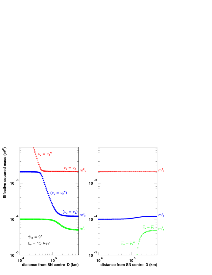
Figure 2: These plots show the effective neutrino masses of neutrinos [Left panel] and antineutrinos [Right panel] inside the star. As visible from $r\to\infty$ regions, we assume that the neutrino spectrum obeys a ‘normal’ mass hierarchy. (We do not emphasize another possibility compatible with the data, ‘inverse’ mass hierarchy. The common mass scale is immaterial for oscillation however.)

At the exit of the star, neutrinos propagate freely as mass eigenstate in vacuum e.g., $\nu_{e}\equiv\nu_{3}$, see Fig. 2 [Left]. This depends on the unknown size of the vacuum mixing angle $\theta_{13}$ ($U_{e3}=\sin\theta_{13}$) and on the electron density distribution in the star $N_{e}\propto\rho Y_{e}$. The approximate values of $\theta_{13}$ when adiabatic conversion should occur are shown in the following equation:

$$P_{ee}=|\langle\nu_{e}|\nu_{e}(t)\rangle|^{2}=\left\{\begin{array}[]{lcl}U_{e3}^{2}\sim 0&\mbox{ if }\theta_{13}>1^{\circ}&\mbox{adiabatic conversion of }\nu_{e}\to\nu_{3}\\ U_{e2}^{2}\sim 0.3&~{}~{}\mbox{ if }\theta_{13}<0.1^{\circ}&\mbox{adiabatic conversion of }\nu_{e}\to\nu_{2}\end{array}\right.$$ (11)

(at present, we cannot exclude that $\theta_{13}$ falls in an intermediate case). Solar neutrino mixing makes almost certainly adiabatic the second conversion, if the first should fail.
Thus, accounting fo oscillations, the fluence of $\nu_{e}$ becomes:

$$F_{\nu_{e}}=\left\{\begin{array}[]{lc}F_{\nu_{x}}^{0}&\mbox{ if }\theta_{13}>1^{\circ}\\ 0.3F_{\nu_{e}}^{0}+0.7F_{\nu_{x}}^{0}&~{}~{}\mbox{ if }\theta_{13}<0.1^{\circ}\end{array}\right.$$ (12)

Similarly, for antineutrinos $\bar{\nu}_{e}=\bar{\nu}_{1}^{m}(t)$, see Fig. 2 [Right], that implies $P_{\bar{e}\bar{e}}=|\langle\bar{\nu}_{e}|\bar{\nu}_{e}(t)\rangle|^{2}=U_{e1}^{2}\sim 0.7$. Thus, the formula for the flux becomes $F_{\bar{\nu}_{e}}=0.7F_{\bar{\nu}_{e}}^{0}+0.3F_{\nu_{x}}^{0}$. Now we can make the argument for oscillations: Since we expect that $F_{\nu_{e}}^{0}\neq F_{\nu_{x}}^{0}$ and $F_{\bar{\nu}_{e}}^{0}\neq F_{\nu_{x}}^{0}$, oscillations should modify the expected supernova neutrinos fluxes. These modifications are large (e.g., the flash yields little in CC: NC events range from 70 to 100 %) and can be observable, but the message that we want to stress here is simply that these effects should be taken into account in order to interpret the SN neutrino signal correctly.

Finally, we consider the ‘earth matter effect’, possible operative if SN neutrinos cross the earth before hitting the detector. We will show that, with the current oscillation parameters, it is not very large. As we saw, in a possible scenario (=normal mass hierarchy, very small $\theta_{13}$) neutrinos exit from the star as $|\nu_{e}\rangle\to|\nu_{2}\rangle$ and $|\bar{\nu}_{e}\rangle\to|\bar{\nu}_{1}\rangle$ due to the MSW effect [13], or in other words,

$$P_{ee}=\sin^{2}\theta_{12}\sim 0.3~{}~{}~{}\mbox{ and }~{}~{}~{}P_{\bar{e}\bar{e}}=\cos^{2}\theta_{12}\sim 0.7$$

If (anti)neutrinos cross the earth in the last stage of their path, new oscillations will occur (since vacuum eigenstates are not eigenstates in the earth matter) and previous expressions will be modified. For constant density (say, earth mantle - $\rho_{\oplus}\approx 4$ g/cm³) the solution of a two-flavor version of Eq. (10) gives:

$$P_{ee}=\sin^{2}\theta_{12}\left[1+\frac{4\varepsilon\cos^{2}\theta_{12}}{(1+\varepsilon)^{2}-4\varepsilon\cos^{2}\theta_{12}}\cdot\sin^{2}\left(\frac{\Delta m^{2}_{12}L}{4E}\sqrt{(1+\varepsilon)^{2}-4\varepsilon\cos^{2}\theta_{12}}\right)\right]$$ (13)

with $\theta_{12}\approx 33^{\circ}$ and $\Delta m^{2}_{12}\sim 7\cdot 10^{-5}$ eV², where

$$\varepsilon=\frac{\sqrt{2}G_{F}N_{e\oplus}}{\Delta m^{2}_{12}/2E}\simeq 9\ \%\ \frac{\rho_{\oplus}/(\mbox{4\ g/cm}^{3})\cdot Y_{e\oplus}/(\mbox{0.5})\cdot E/(20\mbox{ MeV})}{\Delta m^{2}_{12}/(7\cdot 10^{-5}\mbox{ eV}^{2})}$$

For $\bar{\nu}_{e}$, just replace $\theta_{12}\to 90^{\circ}-\theta_{12}$. Earth matter effect is larger than for solar neutrinos, simply because supernova energies are larger, see Eq. (10). This can give rise to spectacular wiggles, especially if large energies events are seen. Numerical considerations based on previous formulae suggest that this investigation will be demanding. If (or when) the position of the supernova will be known, it will be possible to include such an effect, reducing ambiguities in the interpretation of the signal.

2.4 Importance of electron neutrino signal ($\nu_{e}$ absorption on Argon)

In order to complete the discussion and to show an application of the formalism, we will consider in detail the specific supernova neutrino signal provided by the reaction of absorption

$$\nu_{e}+\mbox{Ar}\to\mbox{K${}^{*}$}+e^{-}$$ (14)

that has a large cross-section. The signature for reaction (14) is given by a leading electron accompanied by soft electrons from conversion of K^∗ de-excitation $\gamma$’s in the Argon volume surrounding the interaction vertex. This signal could be seen by the forthcoming detector ICARUS [16] based on the liquid Argon technology. (We are not going to discuss the more difficult and important question of ‘what we can learn from supernova neutrinos’, whose answer will of course depend on which neutrino detectors will be working when next galactic supernova will explode and what will be the distance of this supernova; but it is almost from granted that we will learn a lot from the $\overline{\nu}_{e}p\to ne^{+}$ reaction for the reasons recalled in App. A).

In a 3 kton liquid Argon detector the number of $\nu_{e}$-absorption events is about 400, for a supernova exploding at $D=10$ kpc. To calculate this number, one simply multiplies the fluence (including oscillations) by the number of target nuclei and by the cross-section of the reaction, and than integrates over the possible neutrino energies. In the present calculation we employed a ‘hybrid model’ for the cross-section of the reaction in Eq. (14): shell model for allowed transitions, and random phase approximation (RPA) for forbidden ones (see below). The other inputs were: (a) a normal hierarchy of neutrino masses; (b) $\theta_{13}$ large enough to produce $P_{ee}\sim 0$ – that is, $\nu_{e}\to\nu_{3}$ producing $F_{\nu_{e}}\equiv F^{0}_{\nu_{x}}$; (c) an exact equipartition of the fluxes ($f={1}/{6}$) and ${\cal E}_{B}=3\times 10^{53}\mbox{ erg}$; (d) a spectrum without pinching ($\eta=0$); (e) a neutrino temperature of $T_{\nu_{x}}=5.1$ MeV, corresponding to an average energy $\langle E_{\nu_{x}}\rangle=16$ MeV (following the indications of the most recent calculations [9], we assume that in absence of oscillations the temperature of electron neutrinos is $T_{\nu_{e}}=3.5$ MeV, that is closer to $T_{\nu_{x}}$ than thought in the past).

The use of adequate cross-section for neutrino absorption reaction on Argon is important. Allowed transitions to low lying Potassium (K) excited levels dominate for neutrino energies less than $\sim 15$ MeV (i.e. in the energy range of interest for solar neutrino experiment). Shell model computation [17] allows to reliably describe the allowed cross-section. At higher energies, as for the SN case here considered, forbidden transitions become relevant as well. These are dominated by the collective response to giant resonance, so that the RPA model [18] is usually considered sufficient to describe the non-allowed contributions to the ($\nu_{e}$, Ar) cross-section.

Figure 3: Number of expected $\nu_{e}$ events as a function of the effective temperature. Oscillation are separately accounted for - full line and dotted line - according to the two reference cases of Eq. (12). Neutrino fluence is taken from Eq. (8), with $T$ free to vary and pinching parameter set at $\eta=0$. The other SN parameters are: $D=50$ kpc, $f=1/6$ (strict equipartition), and ${\cal E}_{B}=3\times 10^{53}$ erg. The cross-section ‘hybrid model’ for $\nu_{e}$-absorption on Argon is used. A reference 3 kton detector mass (corresponding to $3\times 1.5\cdot 10^{31}$ Ar targets) is considered. For simplicity, we assume an ideal detector, without threshold on the final state electron energy and full detection efficiency.

How the number of events changes, with reasonable changes of the input parameters? To answer this question, we can calculate the percentage variation $100\times\delta N/N$ of the number of absorbed $\nu_{e}$ under a number of alternative hypotheses:

${T+\Delta T}$	${T-\Delta T}$	${f\to{1}/{8}}$	${\eta\to 2}$	${P_{ee}\to 0.3}$
$+51$ %	${-45}$ %	${-25}$ %	${+15}$ %	${-16}$ %

The first two columns show the effect of changing the temperature by $\Delta T=\pm 1.3$ MeV; the third column, describes the effect of non-equipartitioned fluxes; the fourth one, the effect of having a pinched (‘non-thermal’) spectrum; the last column, assumes that $\nu_{e}\to\nu_{2}$ due to very small $\theta_{13}$. This shows that the present uncertainty in the temperature has a big impact on the expected signal, about $50$ %. It shows also that a mixture of various phenomena can affect the flux at the $\sim 20$ % level. To separate these effects clearly, it will be important to study several properties of the neutrino signal, like distributions in time and energy and use several reactions. In Fig. 3 we show the calculated number of expected events for a wide range of values of the effective temperature.

In some situations, the electron neutrino signal can lead to ‘model independent’ inferences. For instance, if it were possible to demonstrate that the earth matter effect (associated with solar $\Delta m^{2}\approx 7.1\cdot 10^{-5}$ eV²) occurs in $\nu_{e}$ events and in $\bar{\nu}_{e}$ events, we would have a proof that $\theta_{13}$ is small. If instead it occurs only for $\bar{\nu}_{e}$, the converse is true and furthermore, the hierarchy must be normal (there is an adiabatic conversion associated with the heaviest neutrino). It should be remarked however that a ‘golden’ observation (that is seeing one or more wiggles) requires a great precision in energy measurement or a lucky configuration, namely, a supernova exploding just below the horizon. In fact, the phase of oscillation with solar $\Delta m^{2}$ is close to $\pi/2$ for lengths of propagation through the earth of the order of $350\mbox{ km}\times E_{\nu}/(20\mbox{MeV})$, see Eq. (13).

But note that even the absence of a $\nu_{e}$ signal would be a precious information. Indeed, to help the ‘delayed explosion’ to take place, it would be better to have a depletion of $\nu_{x}$ during accretion. In that case, the number of $\nu_{e}$ events in the first half-a-second should be small, due to Eq. (12), whereas they should be seen during cooling. Similarly, if non-standard scenarios (like collapse with rotation) are realized, $\nu_{x}$ can be depleted also during the cooling phase. In this case, $\nu_{e}$ events would be rare even during cooling.

3 Summary and discussion

In this introduction to $\nu$-astronomy, we focused mostly on supernova neutrinos. We aimed at helping the orientation of a reader in this field, so we did not attempt to give a comprehensive study (i.e. we did not consider all theoretical possibilities or scenarios, or reactions to detect neutrinos). Rather, we offered a selection of the background information, provided some few formulae, reference numbers, and showed illustrative calculations. Let us conclude by recalling some of the important points we touched:

$\star$ Neutrino astronomy is theoretically appealing and rich of promises. Supernova neutrinos are a very well defined and interesting possibility.

$\star$ Neutrino observations from SN1987A are not in contradiction with the general theoretical picture. However, supernova explosions are still mysterious, and this warrants more discussion and stimulates more efforts.

$\star$ Next galactic supernova will permit us much more precise observations and this will be certainly very helpful to progress. In particular, the response from new generation neutrino detector(s), sensitive to various types of neutrinos and reactions could be of major importance (we discussed in some detail the case of a detector like ICARUS, that combines a large mass with a high resolution and detection efficiency).

$\star$ The effects of oscillations are important and have to be included. Conversely, one could combine experiments and use theoretical information in order to attempt to make inferences on oscillations, but astrophysical uncertainties should be thought as an essential systematics for this purpose. (In other words, there are chances to learn something on neutrinos, but, in our view, the primary aim of these observations is just supernova astrophysics.)

$\star$ All this is fine; the most important task left is an exercise of patience, $0-100$ years for next galactic supernova.

Appendices

Appendix A An example of cross-section (inverse $\beta$ decay)

The ‘inverse $\beta$-decay’ reaction $\bar{\nu}_{e}+p\to e^{+}+n$ is particularly important for actual neutrino detection. Indeed, it has a large cross-section and water Čerenkov and scintillator based detectors have many free protons. For illustration, we recall here a simple approximation of this reaction (from last paper of Ref. [15]) and refer to [15] for a more complete discussion.

The tree level cross-section in terms of Mandelstam invariants $s,t,u$ is:

$$\frac{d\sigma}{dt}=\frac{G_{F}^{2}\cos^{2}\!\theta_{C}}{2\pi(s-m_{p}^{2})}~{}[A(t)-B(t)(s-u)+C(t)(s-u)^{2}]$$ (A.1)

$A,B,C$ are well approximated as $c_{1}+t\cdot c_{2}$ at the energy of supernova neutrino detection:

$$\begin{array}[]{l}A\approx M^{2}(1-g^{2})(t-m_{e}^{2})-M^{2}\Delta^{2}(1+g^{2})-2m_{e}^{2}M\Delta g(1+\xi)\\ B\approx g(1+\xi)t\\ C\approx(1+g^{2})/4\end{array}$$ (A.2)

where $M=(m_{n}+m_{p})/2$, $\Delta=m_{n}-m_{p}$, $\xi=3.706$ and $g=-1.270\pm 0.003$. Eq. (A.1) is related by Jacobians to the cross-sections differential in the lepton energy $E_{e}$, or in the angle $\theta=0-\pi$ between the incoming neutrino and the charged positron:

$$\frac{d\sigma}{dE_{e}}={2m_{p}}\frac{d\sigma}{dt}~{}~{}~{}\mbox{ and }~{}~{}~{}\frac{d\sigma}{d\cos\theta}=\frac{\epsilon p_{e}}{1+\epsilon(1-\frac{E_{e}}{p_{e}}\cos\theta)}\frac{d\sigma}{dE_{e}}$$ (A.3)

Of course, for the first formula one has to express the Mandelstam variables in terms of $E_{\nu}$ and $E_{e}$, e.g., $t=m_{n}^{2}-m_{p}^{2}-2m_{p}(E_{\nu}-E_{e})$. To evaluate the second formula, one first defines $\epsilon=E_{\nu}/m_{p}$ and calculates the positron energy $E_{e}$ (and momentum $p_{e}$) from $E_{e}=[(E_{\nu}-\delta)(1+\epsilon)+\epsilon\cos\theta((E_{\nu}-\delta)^{2}-m_{e}^{2}k^{2})^{1/2}]/k$, where $\delta=(m_{n}^{2}-m_{p}^{2}-m_{e}^{2})/(2m_{p})$ and $k=(1+\epsilon)^{2}-(\epsilon\cos\theta)^{2}$. Note that $E_{\nu}$ is one-to-one with $E_{e}$ at zeroth order in $\epsilon$. The threshold of the reaction is at $E_{\nu}>1.806$ MeV.

Appendix B Fermi integrals and polylog

Let us consider the function $f_{n}(x,\eta)$ where $n=1,2,3...$ and $\eta$ is a real parameter:

$$f_{n}(x,\eta)=\frac{x^{n}}{1+e^{x-\eta}}~{}~{}~{}\mbox{with}~{}~{}x\geq 0$$

This function is needed to define the Fermi integral of $n$-th order as follows:

$$F_{n}(\eta)\equiv\int^{\infty}_{0}f_{n}(x,\eta)~{}dx=-{\rm Li}_{n+1}(-e^{\eta})\cdot n!$$ (B.1)

The last expression involves the polylogarithm function ${\rm Li}_{n}(x)$.

$\bullet$ This integral appears commonly when using the Fermi-Dirac distribution, that can be written as $T^{2}f_{2}(x,\eta)$, with $x=E/T$. E.g., integrating this distribution for all values of the energy $E$ we get the normalization factor of Eq. (6) of Sec.2.2:

$$\int^{\infty}_{0}T^{2}f_{2}(x,\eta)~{}dE~{}=~{}T^{3}~{}F_{2}(\eta)$$ (B.2)

$\bullet$ Eq. (B.1) is also useful to express energy momenta:

$$\langle E\rangle=T\cdot\frac{F_{3}(\eta)}{F_{2}(\eta)},~{}~{}\ \ \langle E^{2}\rangle=T^{2}\cdot\frac{F_{4}(\eta)}{F_{2}(\eta)},~{}~{}\ \ \langle\delta E\rangle\equiv\sqrt{\langle E^{2}\rangle-\langle E\rangle^{2}}$$ (B.3)

The variance $\langle\delta E\rangle$ stays constant at better than 0.2 % for $\eta<5$ at the value $\langle\delta E\rangle=1.73\cdot T$. A useful approximate expression for the average energy $\langle\delta E\rangle$ can be obtained using ${\rm Li}_{4}(-1+y)/{\rm Li}_{3}(-1+y)-1\approx(50.5-41.8y-6.4y^{2}-2.3y^{3})/1000$, where we have in mind the identification $y\equiv 1-\exp(-\eta)$.

$\bullet$ For $\eta=0,1,2$ we get $F_{2}=1.803,4.328,9.513$ and $F_{3}=5.682,14.39,34.30$.

$\bullet$ The series expansion ${\rm Li}_{n}(z)=\sum_{m=1}^{\infty}z^{m}/m^{n}$ of the polylog leads to some identities:

$${\rm Li}_{0}(z)=z/(1-z);\ \ ~{}~{}~{}{\rm Li}_{1}(z)=-\log(1-z);\ \ ~{}~{}~{}{\rm Li}_{n+1}(z)=\int_{0}^{z}{\rm Li}_{n}(\tau)\frac{d\tau}{\tau}\ \mbox{with }z>0$$ (B.4)

$\bullet$ At $z=\pm 1$, the polylogarithm can be expressed by the Z-function (See Eq. (B.1)):

$$\begin{array}[]{lr}{\rm Li}_{n}(1)=Z_{n},&(Z_{2,3,4,5}=1.645,1.202,1.082,1.037)\\ {\rm Li}_{n}(-1)=-(1-2^{1-n})Z_{n}&\qquad\qquad\qquad\mbox{(connection of Bose and Fermi integrals)}\end{array}$$ (B.5)

Appendix C A reminder on neutrino masses and oscillations

(1) The mixing matrix $U$ (introduced by Sakata and collaborators in 1962) connects neutrino fields of given flavor and of given mass:

$$\nu_{\ell}(x)=U_{\ell i}\ \nu_{i}(x),~{}~{}\mbox{ where }\ell=e,\mu,\tau\mbox{ and }i=1,2,3$$ (C.1)

This implies a relation between states of ultrarelativistic neutrinos. In fact, the decomposition in oscillators $\nu(x)=\sum_{p\lambda}(a_{p\lambda}u_{p\lambda}e^{ipx}+b_{p\lambda}^{\dagger}v_{p\lambda}e^{-ipx})$ implies $b_{\ell}^{\dagger}=U_{\ell i}b_{i}^{\dagger}$ and $a_{\ell}^{\dagger}=U_{\ell i}^{*}a_{i}^{\dagger}$, so:

$$\begin{array}[]{l}|\nu_{\ell}\rangle=U_{\ell i}^{*}|\nu_{i}\rangle\\ |\bar{\nu}_{\ell}\rangle=U_{\ell i}|\bar{\nu}_{i}\rangle\end{array}$$ (C.2)

No change if the type of mass is Dirac instead than Majorana (last one being theorist’s favorite).

(2) From previous considerations, it follows that if we produce a state of flavor $\ell$ at $t=0$ it will acquire overlap with other states at later time (“appearance” of a new flavor) and at the same time it will loose overlap with itself (“disappearance”). This was shown by B.Pontecorvo in 1967, though, the first idea dates back to 1957. Thus, a state with momentum $p$ becomes

$$|\nu_{\ell}(t)\rangle=U_{\ell i}^{*}|\nu_{i}(t)\rangle,~{}~{}~{}\mbox{ where }|\nu_{i}(t)\rangle=e^{i(px-E_{i}t)}\ |\nu_{i}(0)\rangle$$ (C.3)

The energy of neutrinos with different masses cannot remain the same in the course of the propagation, since $E_{i}\approx p+m_{i}^{2}/(2p)$ (ultrarelativistic approximation always applies to the cases of interest). When the distance between production and detection satisfies $L\approx t\gg E/\Delta m_{ij}^{2}$, $|\nu_{\ell}(t)\rangle$ becomes different from $|\nu_{\ell}(0)\rangle$, if the mixings $U_{\ell i}$ are large enough. As usual, $\Delta m^{2}_{ij}=m_{j}^{2}-m_{i}^{2}$.

(3) The effective hamiltonian of propagation in vacuum is $U{\rm diag}(m_{i}^{2})U^{\dagger}/2E$ (for antineutrinos, $U\to U^{*}$), but in matter there is an additional term $\pm\sqrt{2}G_{F}N_{e}{\rm diag}(1,0,0)$ ($+$ is for $\nu_{e}$, $-$ for $\bar{\nu}_{e}$; $N_{e}=\rho Y_{e}/m_{n}=e^{-}$ number density). This term is linear in the Fermi coupling. It describes a coherent interaction of neutrinos with the matter where it propagates. This can drive neutrinos to be “local” mass eigenstates during the propagation, thus exiting from a star as vacuum eigenstates, i.e.: $|\nu_{e}\rangle\to|\nu_{2}\rangle$ or $|\nu_{e}\rangle\to|\nu_{3}\rangle$. In the sun, this effect (named after MSW after Wolfenstein, Mikheyev and Smirnov [13]) is partial and it is pronounced for highest energy neutrino events, e.g., the CC events at SNO. In the supernova, it can be complete.

(4) Putting aside the indications of LSND indication (that will be tested at MiniBooNE) we know from a number of experiments that the usual 3 neutrino flavors most likely oscillate among them and this points to the following (roughly 1 sigma) ranges of the parameters [19]:

$$\begin{array}[]{lll}\Delta m^{2}_{12}=7.1\pm 0.7\cdot 10^{-5}\mbox{ eV}^{2};{}{}{}&\theta_{12}=33^{\circ}\pm 2^{\circ}&\\ \Delta m^{2}_{23}=2.0\pm 0.4\cdot 10^{-3}\mbox{ eV}^{2};{}{}{}&\theta_{23}=45^{\circ}\pm 7^{\circ};{}{}&\theta_{13}<9^{\circ}\end{array}$$ (C.4)

The 3 mixing angles given above parameterize the unitary mixing matrix $U_{\ell i}$:

$$|U_{e3}|=\sin\theta_{13},\ \ |U_{e2}/U_{e1}|=\tan\theta_{12}\ (\mbox{solar mix.}),\ \ |U_{\mu 3}/U_{\tau 3}|=\tan\theta_{23}\ (\mbox{atmospheric mix.}).$$

(5) We have some bounds on neutrino masses (in this sense, we know something more than the oscillation parameters $\Delta m^{2}_{ji}$) from other sources: from $\beta$-decay (Mainz, Troitsk), $\sqrt{\sum_{i}|U_{ei}^{2}|m_{i}^{2}}\leq 2.2$ eV; from neutrinoless double beta decay (Heidelberg-Moscow at Gran Sasso, IGEX), $|\sum_{i}U_{ei}^{2}m_{i}|\leq 0.3-1$ eV [a claim was made that the transition has been observed, but in our opinion, with a weak significance]; from galaxy surveys (2dF) $\sum_{i}m_{i}<1.8$ eV or combined cosmological results (including WMAP) $\sum_{i}m_{i}<0.7$ eV. We do not discuss them further, but we note that they suggest that the kinematic search of effects of neutrino masses with SN neutrinos is difficult or impossible.

References

-
[1]
E.g., SPIRES database
http://www-spires.slac.stanford.edu/spires/hep/;
NASA/ESO database
http://esoads.eso.org/abstract_service.html - [2] See SPIRES in previous entry and the PaNAGIC site at http://www.lngs.infn.it/
- [3] T. Montaruli, “MACRO as a telescope for neutrino astronomy,” ICRC99, vol.2, 213, hep-ex/9905020 (see in particular tables 2 and 3)
- [4] F. Halzen and D. Hooper, “High-energy neutrino astronomy: The cosmic ray connection,” Rept. Prog. Phys. 65 (2002) 1025
- [5] K. Hirata et al. [KAMIOKANDE-II Coll.], Phys. Rev. Lett. 58 (1987) 1490 and Phys. Rev. D 38 (1988) 448; R.M. Bionta et al. [IMB Coll.] Phys. Rev. Lett. 58 (1987) 1494; E.N. Alekseev et al. [Baksan Coll.] JETP Lett. 45 (1987) 589 and Phys. Lett. B 205 (1988) 209
- [6] R. Barbon, V. Buondí, E. Cappellaro, M. Turatto, Astronomy and Astrophysics 139 (1999) 531 and the Padova-Asiago Supernova database at the site http://merlino.pd.astro.it/supern/
- [7] M. Malek et al. [Super-Kamiokande Coll.], Phys. Rev. Lett. 90 (2003) 061101
- [8] J.F. Beacom and M.R. Vagins, hep-ph/0309300
- [9] See for instance the reviews by H.A. Bethe and J.R. Wilson, “Revival of a stalled supernova shock by neutrino heating,” Astrophys. J. 295 (1985) 14; H.A. Bethe, Rev. Mod. Phys. 62 (1990) 801. H.T. Janka et al., “Explosion mechanisms of massive stars,” astro-ph/0212314
- [10] H.T. Janka et al., “Neutrinos from type II supernovae and the neutrino driven supernova mechanism,” Vulcano 1992 Proceedings, page 345-374
- [11] See e.g., the reviews of V.S. Imshennik published in Astronomy Letters, 18, (1992) 489 and Space Science Reviews 74 (1995) 325 and C.L. Fryer and A. Heger, Astrophys. J. 541 (2000) 1033 (in particular Fig.12).
- [12] T.J. Loredo and D.Q. Lamb, “Bayesian analysis of neutrinos observed from supernova SN 1987A,” Phys. Rev. D 65 (2002) 063002
- [13] L. Wolfenstein, “Neutrino oscillations in matter,” Phys. Rev. D 17 (1978) 2369; S.P. Mikheev and A.Yu. Smirnov, “Resonance enhancement of oscillations in matter and solar neutrino spectroscopy,” Sov. J. Nucl. Phys. 42 (1985) 913. See also V.D. Barger, K. Whisnant, S. Pakvasa and R.J. Phillips, “Matter effects on three-neutrino oscillations,” Phys. Rev. D 22 (1980) 2718. Analytical formulae suited for supernova neutrinos are given in G.L. Fogli, E. Lisi, D. Montanino and A. Palazzo, Phys. Rev. D 65 (2002) 073008 [E-ibid. D 66 (2002) 039901].
- [14] G. Dutta, D. Indumathi, M. V. Murthy and G. Rajasekaran, Phys. Rev. D 61 (2000) 013009; A.S. Dighe and A.Yu. Smirnov, Phys. Rev. D 62 (2000) 033007; C. Lunardini and A.Yu. Smirnov, Nucl. Phys. B 616 (2001) 307 and hep-ph/0302033; K. Takahashi, M. Watanabe, K. Sato and T. Totani, Phys. Rev. D 64 (2001) 093004 M. Kachelrieß, A. Strumia, R. Tomas and J.W.F. Valle, Phys. Rev. D 65 (2002) 073016; V. Barger, D. Marfatia and B.P. Wood, Phys. Lett. B 532 (2002) 19; M. Aglietta et al., hep-ph/0307287
- [15] C.H. Llewellyn Smith, “Neutrino reactions at accelerator energies,” Phys. Rept. 3 (1972) 261; P. Vogel and J.F. Beacom, “The angular distribution of inverse beta decay, ,” Phys. Rev. D 60 (1999) 053003; A. Strumia and F. Vissani, “Precise quasielastic neutrino nucleon cross-section,” Phys.Lett. B 564 (2003) 42
- [16] F. Arneodo et al. [ICARUS Coll.], “The ICARUS Experiment”, LNGS-EXP 13/89 add. 2/01 (Nov. 2001). See also http://www.aquila.infn.it/icarus/ for a complete list of references
- [17] W.E. Ormand et al., “Neutrino Capture cross-sections for 40Ar and -decay of 40Ti”, Phys.Lett. B345 (1995) 343
- [18] E. Kolbe, K. Langanke and G. Martinez-Pinedo, private communication
- [19] See e.g., G.L. Fogli et al. hep-ph/0308055; P. Creminelli et al., hep-ph/0102234 that is updated after new data