The traditional approximation in general relativity

Abstract

We discuss the generalisation of the so-called traditional approximation, well known in geophysics, to general relativity. We show that the approximation is applicable for rotating relativistic stars provided that one focuses on relatively thin radial shells. This means that the framework can be used to study waves in neutron star oceans. We demonstrate that, once the effects of the relativistic frame-dragging are accounted for, the angular problem reduces to Laplace’s tidal equation. We derive the dispersion relation for various classes of waves in a neutron star ocean and show that the combined effects of the frame-dragging and the gravitational redshift typically lower the frequency of a mode by about 20%.

1 Motivation

Accreting neutron stars exhibit a variety of quasiperiodic phenomena, with frequencies ranging from a few Hz to well above 1 kHz. Many of the observed oscillations are likely associated with processes in the accretion disk, but it is also probable that some of the observed features are linked to waves in the neutron star ocean (Bildsten and Cutler, 1995; Heyl, 2001; Strohmayer and Bildsten, 2003). For example, it has been observed that neutron stars that accrete matter at rates $\gtrsim 10^{-9}M_{\odot}\mathrm{yr}^{-1}$(the so-called Z-sources) show quasi-periodic oscillations with frequencies of $\sim 6$ Hz. It has also been argued that the Z-sources are covered by massive oceans comprising a mass of $\sim 10^{-6}M_{\odot}$ composed of a degenerate liquid of light elements (C, O, Ne, Mg,..). This led Bildsten and Cutler (1995) to argue that the observed oscillations may correspond to ocean g-modes.

To analyse this suggestion in more detail Bildsten, Ushomirsky and Cutler (1996) investigated the nature of low-frequency waves in the ocean of a rotating neutron star. They considered slowly rotating stars (far below the breakup limit) in Newtonian gravity, and made use of the assumption that $\Omega\gg\sigma$, where $\Omega$ is the rotation frequency and $\sigma$ is the mode frequency. This is a reasonable assumption since neutron stars accreting at a high rate are expected to spin much faster than a few Hz. The studies of Bildsten and Cutler (1995) and Bildsten, Ushomirsky and Cutler (1996) both made use of the so-called “traditional” approximation, which has its origins in geophysics. This approximation leads to a separation of variables for the linearised Euler equations, where the angular problem is described in terms of Laplace’s tidal equation. The solutions to this equation have been discussed in detail by many authors (Müller, Kelly and O’ Brien, 1993; Miles, 1977; Bildsten, Ushomirsky and Cutler, 1996; Lee and Saio, 1997; Townsend, 2003).

The purpose of this paper is to extend the “traditional approximation” to general relativity. The main motivation for this is that we know from the studies of Bildsten and Cutler (1995); Bildsten, Ushomirsky and Cutler (1996) Townsend (2003) that the approximation provides a relatively simple way of analysing ocean waves in rotating Newtonian stars. Yet there are several reasons for studying this problem in the framework of general relativity. First of all, neutron stars are highly relativistic objects with $GM/Rc^{2}\approx 0.15-0.2$. This means that one must account for the gravitational redshift when comparing observed oscillations to theoretical models. A second relativistic effect that needs to be accounted for is the rotational frame-dragging. Finally, the traditional approximation scheme is interesting from a conceptual point of view. Especially since it provides an alternative approach to existing work on the low-frequency oscillations of rotating relativistic stars (see Lockitch, Friedman and Andersson (2003) for a discussion and references to the relevant literature).

2 The relativistic equations of motion

We begin by deriving the equations that govern a small amplitude ocean wave on a relativistic star. We consider a star which rotates uniformly at frequency $\Omega\ll(GM/R^{3})^{1/2}$, where $M$ and $R$ are the neutron star mass and radius. This means that the star rotates at a small fraction of the break-up velocity, allowing us to neglect the “centrifugal force” and treat the unperturbed star as spherical. This approximation is justified for most observed neutron stars. However, it is imperative to account for the Coriolis force. In particular since it leads to the existence of a new class of oscillation modes, the so-called “inertial modes” (Provost, Berthomieu and Rocca, 1981; Lockitch, Friedman and Andersson, 2003).

The spacetime of a slowly rotating star is described by the metric

$$ds^{2}=-e^{\nu}dt^{2}+e^{\lambda}dr^{2}-2\omega r^{2}\sin^{2}\theta dt\,d\varphi+r^{2}(d\theta^{2}+\sin^{2}\theta d\varphi^{2}),$$ (1)

where $\omega$ represents the dragging of inertial frames (Hartle, 1967). Physically, $\omega$ represents the angular velocity of a “zero-angular momentum observer” (for which the associated specific angular momentum, $u_{\varphi}$, vanishes) relative to infinity. For an observer co-moving with the fluid, the four-velocity moves on wordlines of constant $t$ and $\theta$, and the corresponding angular velocity $\Omega$ is defined as the ratio

$$\Omega=\frac{u^{\varphi}}{u^{t}}=\frac{d\varphi}{dt}.$$ (2)

Combining this with the requirement that

$$u^{\mu}\,u_{\mu}=-1$$ (3)

we have

$$u^{\mu}=[e^{-\nu/2},0,0,\Omega e^{-\nu/2}].$$ (4)

We wish to consider small perturbations of the star. Since we are mainly interested in ocean waves we will use the Cowling approximation; i.e. assume that all metric perturbations can be neglected. This is a reasonable assumption given the relatively low density of a neutron star ocean. One would, for example, not expect the ocean waves to radiate appreciable amounts of gravitational waves. We also need to neglect the dynamic nature of spacetime if we want to implement the “traditional approximation” in general relativity.

In order to derive the equations that govern the fluid motions we assume that the stellar background is appropriately described by a perfect fluid equation of state with $p=p(\rho)$, which means that the energy-momentum tensor takes the form

$$T^{\mu\nu}=\rho u^{\mu}u^{\nu}+pq^{\mu\nu},$$ (5)

where $q^{\mu\nu}$ is the projection orthogonal to $u^{\mu}$;

$$q^{\mu\nu}=g^{\mu\nu}+u^{\mu}u^{\nu}$$ (6)

and the scalars $\rho$ and $p$ denote the energy density and pressure, as measured by a co-moving observer (an observer with four-velocity $u^{\mu}$), respectively.

The equations of motion follow from the conservation law

$$\nabla_{\mu}T^{\mu\,\nu}=0,$$ (7)

as well as the Einstein field equations. It is well-known that, in the case of slow-rotation, this problem reduces to the standard Tolman-Oppenheimer-Volkoff equations for a non-rotating star, plus a single ordinary differential equation determining the frame-dragging (Hartle, 1967). These equations can be written

$$\lambda^{\prime} = -{2e^{\lambda}(M-4\pi\rho r^{3})\over r^{2}},$$ (8)

$$\nu^{\prime} = {2e^{\lambda}(M+4\pi pr^{3})\over r^{2}}$$ (9)

$$p^{\prime} = -{p+\rho\over 2}\nu^{\prime},$$ (10)

where primes denote derivatives with respect to $r$, and $M=M(r)$ is the “mass within radius $r$”, which follows from the relation

$$e^{\lambda}=\left(1-{2M\over r}\right)^{-1}\ .$$ (11)

To incorporate the leading order rotational effects, we need to solve an additional equation that describes the frame-dragging, $\omega$. It is convenient to use the difference $\tilde{\omega}=\Omega-\omega$, corresponding to the rotation frequency as measured by local zero-angular momentum observers, which is determined by the equation

$$\left[e^{-(\nu+\lambda)/2}\tilde{\omega}^{\prime}\right]^{\prime}+{4\over r}e^{-(\nu+\lambda)/2}\tilde{\omega}^{\prime}-16\pi(p+\rho)e^{(\lambda-\nu)/2}\tilde{\omega}=0\ ,$$ (12)

We also need boundary conditions for $\tilde{\omega}$ at the origin and spatial infinity. At the origin we require that $\tilde{\omega}$ is regular. In the vacuum outside the star, equation (12) can be solved analytically, and we have

$$\tilde{\omega}=\Omega-{2J\over r^{3}},$$ (13)

where $J$ is the total angular momentum of the star. This relation can be used to provide boundary conditions for $\tilde{\omega}$ (and its derivative) at the surface of the star in terms of $\Omega$ and $J$. Specifically, the solution to equation (12) is normalised by requiring that

$$\tilde{\omega}(R)+{R\tilde{\omega}^{\prime}(R)\over 3}=\Omega\ .$$ (14)

In order to derive the equations that govern perturbations, it is useful to work with projections of equation (7) along, and orthogonal to, the four-velocity, cf. Ipser and Lindblom (1992). Projecting along $u^{\mu}$ we have the relativistic continuity equation

$$u^{\mu}\nabla_{\mu}\rho+(p+\rho)\nabla_{\mu}u^{\mu}=0.$$ (15)

The orthogonal projection leads to the relativistic Euler equations

$$(p+\rho)u^{\mu}\nabla_{\mu}u_{\nu}+q^{\mu}_{\nu}\nabla_{\mu}p=0.$$ (16)

Perturbing equation (15), assuming that the Cowling approximation is made (i.e. taking $\delta g_{\mu\nu}=0$), we get

$$\delta u^{\mu}\nabla_{\mu}\rho+u^{\mu}\nabla_{\mu}\delta\rho+(\rho+p)\nabla_{\mu}\delta u^{\mu}=0.$$ (17)

Meanwhile, the perturbed Euler equations can be written as

$$(\delta\rho+\delta p)u^{\mu}\nabla_{\mu}u^{\kappa} + (p+\rho)\delta u^{\mu}\nabla_{\mu}u^{\kappa}+(g^{\nu\kappa}+u^{\nu}u^{\kappa})\nabla_{\nu}\delta p+(p+\rho)u^{\mu}\nabla_{\mu}\delta u^{\kappa}$$ (18)

$$- \delta u^{\nu}u^{\mu}u^{\kappa}(p+\rho)\nabla_{\mu}u_{\nu}=0.$$

The perturbed fluid velocity has (quite generally) components

$$\delta u^{t} = (\Omega-\omega)r^{2}\sin^{2}\theta e^{-\nu/2}H_{2}e^{i(\sigma t+m\varphi)},$$ (19)

$$\delta u^{r} = e^{\nu/2}We^{i(\sigma t+m\varphi)},$$ (20)

$$\delta u^{\theta} = e^{\nu/2}H_{1}e^{i(\sigma t+m\varphi)},$$ (21)

$$\delta u^{\varphi} = e^{\nu/2}H_{2}e^{i(\sigma t+m\varphi)},$$ (22)

where $\delta u^{t}$ has been fixed by the requirement that the overall four-velocity $u^{\mu}+\delta u^{\mu}$ is normalised in the standard way. Here $W$, $H_{1}$ and $H_{2}$ are functions of $r$ and $\theta$, and $\sigma$ is the oscillation frequency observed in the inertial frame. In addition we let

$$\delta p = p_{1}e^{i(\sigma t+m\varphi)},$$ (23)

$$\delta\rho = \rho_{1}e^{i(\sigma t+m\varphi)}.$$ (24)

where $p_{1}$ and $\rho_{1}$ are functions of $r$ and $\theta$. Given these definitions, the continuity equation (17) leads to

$$i(\sigma+m\Omega)\rho_{1} + (p+\rho)e^{\nu}W^{\prime}+\left[(p+\rho)\left({\lambda^{\prime}\over 2}+\nu^{\prime}+{2\over r}\right)+\rho^{\prime}\right]e^{\nu}W$$ (25)

$$+ (p+\rho)e^{\nu}\left[{\partial H_{1}\over\partial\theta}+{\cos\theta\over\sin\theta}H_{1}\right]+im(p+\rho)e^{\nu}H_{2}=0$$

The $r$-component of (18) gives

$$2\,r\left(\rho+p\right)\left[r\left(\omega-\Omega\right)\nu^{\prime}-\omega^{\prime}r+2\,(\Omega-\,\omega)\right]\sin^{2}\theta H_{2}$$

$$-2\,p_{1}^{\prime}-\left(p_{1}+\rho_{1}\right)\nu^{\prime}-2i(\sigma+m\Omega)\,\left(\rho+p\right){e^{\lambda}}W=0,$$ (26)

while the $\theta$ and $\varphi$ components lead to, respectively,

$$2\,\left(\rho+p\right){r}^{2}\left(\Omega-\omega\right)\cos\theta\sin\theta H_{2}-{\frac{\partial p_{1}}{\partial\theta}}-i(\sigma+m\Omega)\,\left(\rho+p\right){r}^{2}H_{1}=0,$$ (27)

and

$$2(p+\rho)r^{2}(\Omega-\omega)\sin\theta\cos\theta H_{1} + imp_{1}+i(\sigma+m\Omega)(p+\rho)r^{2}\sin^{2}\theta H_{2}$$ (28)

$$+ (p+\rho)[(\Omega-\omega)(2r-r^{2}\nu^{\prime})-r^{2}\omega^{\prime}]\sin^{2}\theta W=0.$$

It is worth emphasising the following point: In deriving the above equations we have neglected terms proportional to $\sigma\Omega$ in the $\varphi$-component of the continuity equation (18). Such an approximation is not required in the Newtonian case, as the terms that we have omitted are post-Newtonian contributions. Specifically, the complete $\varphi$-component of equation (18) includes the term

$$i\dfrac{\sigma(\Omega-\omega)}{c^{2}}r^{2}\sin^{2}\theta p_{1}$$

where we have reinstated the speed of light ($c$). This term vanishes in the Newtonian limit ($c\rightarrow\infty)$, but in the relativistic case we can neglect it only when $\sigma$ is suitably small.

We do not, however, expect this difference between the Newtonian and the relativistic equations to have great effect on the ocean waves that we are interested in. The main reason for this is that: i) the Newtonian results show that the g-modes of the ocean have frequencies that scale as $\sqrt{\Omega}$ (Bildsten, Ushomirsky and Cutler, 1996), and ii) inertial modes, like the r-modes, would have frequencies of order $\Omega$ (Lockitch, Friedman and Andersson, 2003). In other words, at least for these classes of modes, our equations should be consistent.

3 The traditional approximation

We now wish to analyse the various oscillation modes of a neutron star ocean. To do this we follow e.g. Bildsten, Ushomirsky and Cutler (1996) and introduce the traditional approximation. As in the Newtonian problem, this corresponds to

• neglecting the Coriolis term in the $r$-momentum equation,

• assuming that the mode is mainly horisontal.

In our case, the first assumption corresponds to neglecting the $H_{2}$ term in equation (26), while the second implies that we should neglect $W$ in equation (28).

With these simplifications equations (27) and (28) can be solved for $H_{1}$ and $H_{2}$. This then gives us

$$-i(\sigma+m\Omega)(p+\rho)r^{2}\sin\theta(1-q^{2}\cos^{2}\theta)H_{1}=\sin\theta{\partial p_{1}\over\partial\theta}+mq\cos\theta p_{1}$$ (29)

and

$$-(\sigma+m\Omega)(p+\rho)r^{2}\sin\theta(1-q^{2}\cos^{2}\theta)H_{2}=2q\sin\theta\cos\theta{\partial p_{1}\over\partial\theta}+mp_{1}$$ (30)

Here we have introduced

$$q={2(\Omega-\omega)\over\sigma+m\Omega}\ .$$ (31)

By using the above results in (25) we find

$$i(\sigma+m\Omega)\rho_{1}+(p+\rho)e^{\nu}W^{\prime}+\left[(p+\rho)\left({\lambda^{\prime}\over 2}+\nu^{\prime}+{2\over r}\right)+\rho^{\prime}\right]e^{\nu}W=-{ie^{\nu}\over(\sigma+m\Omega)r^{2}}L(p_{1}),$$ (32)

where we have defined the operator

$$L={\partial\over\partial\mu}\left({1-\mu^{2}\over 1-q^{2}\mu^{2}}{\partial\over\partial\mu}\right)-{m^{2}\over(1-\mu^{2})(1-q^{2}\mu^{2})}-{mq(1+q^{2}\mu^{2})\over(1-q^{2}\mu^{2})^{2}},$$ (33)

with $\mu=\cos\theta$. Notably, this has exactly the same form as the angular operator in the Newtonian problem, cf. equation (7) in Bildsten, Ushomirsky and Cutler (1996). One has to be careful here, though, because in the relativistic case $L$ depends on $r$ through $q$ (which in turn depends on $\omega(r)$). However, as long as we are interested in oscillations in a thin radial shell we may take the frame-dragging to be a constant.

Aiming to write the final equations in a form reminiscent of the Newtonian results, we relate the displacement component $\xi^{r}$ to the perturbed velocity component via

$$\delta u^{\mu}=q^{\mu}_{\ \nu}\pounds_{u}\xi^{\nu},$$ (34)

where the projection $q^{\mu\nu}$ was defined earlier, and where $\pounds_{u}$ is the Lie derivative along $u^{\mu}$ This means that

$$\xi^{r} = \dfrac{e^{\nu}\,W(r,\theta)e^{i(\sigma t+m\phi)}}{i(\sigma+m\Omega)},$$ (35)

$$\xi^{\theta} = \dfrac{e^{\nu}\,H_{1}(r,\theta)e^{i(\sigma t+m\phi)}}{i(\sigma+m\Omega)},$$ (36)

$$\xi^{\phi} = \dfrac{e^{\nu}\,H_{2}(r,\theta)e^{i(\sigma t+m\phi)}}{i(\sigma+m\Omega)}.$$ (37)

We have used the inherent gauge freedom to set the temporal displacement to zero, i.e. $\xi^{t}=0$. We also relate the Eulerian perturbations in density and pressure in the standard way;

$${\Delta p\over\Gamma_{1}p}={\Delta\rho_{1}\over p+\rho}\Rightarrow\dfrac{p_{1}+\xi^{\mu}p_{\,;\,\mu}}{\Gamma_{1}p}=\dfrac{\rho_{1}+\xi^{\mu}\rho_{\,;\,\mu}}{\rho+p}\Rightarrow\rho_{1}={p+\rho\over\Gamma_{1}p}p_{1}-\xi^{r}\left[\rho^{\prime}-{p+\rho\over\Gamma_{1}p}p^{\prime}\right],$$ (38)

where $\Gamma_{1}$ is the adiabatic exponent $\Gamma_{1}=\left(\dfrac{\partial\ln p}{\partial\ln\rho}\right)$ evaluated at constant entropy.

Given these various relations we can write equation (32) as

$$-\xi^{r\prime}-\left[{p_{1}\over\Gamma_{1}p}+\left({p^{\prime}\over\Gamma_{1}p}+{\lambda^{\prime}\over 2}+{2\over r}\right)\xi^{r}\right]={pe^{\nu}\over(\sigma+m\Omega)^{2}r^{2}(p+\rho)}L\left({p_{1}\over p}\right)$$ (39)

Finally, the $r$-momentum equation (26) reads (after neglecting the Coriolis term) :

$$(p+\rho)e^{\lambda-\nu}\left[(\sigma+m\Omega)^{2}+{\nu^{\prime}e^{\nu-\lambda/2}\over 2}\mathcal{A}\right]\xi^{r}=p_{1}^{\prime}+{\nu^{\prime}\over 2\Gamma_{1}p}\left[\rho+(1+\Gamma_{1})p\right]p_{1},$$ (40)

where we have defined the relativistic Schwarzschild discriminant as

$$\mathcal{A}={e^{-\lambda/2}\over p+\rho}\left(\rho^{\prime}-{p+\rho\over\Gamma_{1}p}p^{\prime}\right).$$ (41)

For later convenience, we also introduce the relativistic analogue of the Brunt-Väisälä frequency as

$$N^{2}=-\dfrac{\nu^{\prime}}{2}\mathcal{A}$$ (42)

.

4 The Newtonian limit

As a consistency check of our derivation we want to compare our final formulas (39) and (40) to the corresponding results in the Newtonian case. To facilitate this comparison we need to transform our expressions, which are determined in a coordinate basis, into an orthonormal basis. This basis should be the relativistic analogue of the flat space-time orthonormal basis used by Bildsten, Ushomirsky and Cutler (1996);

$$\vec{\xi}_{\mathrm{N}}=\xi^{r}_{\mathrm{N}}\hat{r}+\xi^{\theta}_{\mathrm{N}}\hat{\theta}+\xi^{\varphi}_{\mathrm{N}}\hat{\varphi},$$ (43)

where the subscript $\mathrm{N}$ denotes a Newtonian vector.

In the corresponding relativistic basis, the spatial components $\xi^{a}_{\mathrm{o}}$ of the displacement vector are determined from

$$\xi^{r}_{\mathrm{o}} = e^{\lambda/2}\xi^{r}\ ,$$ (44)

$$\xi^{\theta}_{\mathrm{o}} = r\xi^{\theta}\ ,$$ (45)

$$\xi^{\phi}_{\mathrm{o}} = r\sin\theta\xi^{\phi}\ ,$$ (46)

In this frame we can identify the components of the displacement with their Newtonian counterparts. Moreover, we can argue in favour of the validity of the traditional approximation in a way analogous to that of Bildsten, Ushomirsky and Cutler (1996).

In the orthonormal frame equation (26) becomes

$$e^{-\nu+\lambda/2}\left[(\sigma+m\Omega)^{2}+\dfrac{\nu^{\prime}e^{\nu-\lambda/2}}{2}\mathcal{A}\right]\xi^{r}_{\mathrm{o}}=p_{1}^{\prime}+{\nu^{\prime}\over 2}\left(\dfrac{\rho+p}{p\Gamma_{1}}+1\right)p_{1}$$

$$+ie^{-\nu}(\sigma+m\Omega)\left[(\Omega-\omega)\left(r\nu^{\prime}+2\right)+r\omega^{\prime}\right]\sin\theta\xi^{\varphi}_{\mathrm{o}}.$$ (47)

We can safely neglect the Coriolis term (the last term of the right-hand side) as long as

$$\left|N^{2}\xi^{r}_{\mathrm{o}}\right|\gg e^{-\nu}(\sigma+m\Omega)\left|\left[(\Omega-\omega)\left(r\nu^{\prime}+2\right)+r\omega^{\prime}\right]\sin\theta\xi^{\varphi}_{\mathrm{o}}\right|\ ,$$ (48)

or equivalently

$$\left|N^{2}\right|\gg(\sigma+m\Omega)\left|\left[(\Omega-\omega)\left(r\nu^{\prime}+2\right)+r\omega^{\prime}\right]\right|\left|\dfrac{\xi^{\varphi}_{\mathrm{o}}}{\xi^{r}_{\mathrm{o}}}\right|.$$ (49)

Since we are assuming that the mode is horisontal, it is far from obvious that this inequality will hold. However, for a neutron star ocean the order of magnitude of $r\omega^{\prime}$ can be estimated from the value at the surface. From equation (14), we see that

$$r\omega^{\prime}\approx R\tilde{\omega}^{\prime}(R)=3\tilde{\omega}(R)\approx\dfrac{6I\Omega}{R^{3}}\approx\dfrac{12M\Omega}{5R}$$ (50)

and since $M/R\approx 1/5$ for a typical neutron star it follows that $r\omega^{\prime}\approx\dfrac{12}{25}\Omega$. In a similar way,

$$\nu^{\prime}\approx{2e^{\lambda}M\over r^{2}}\approx{2M\over R^{2}}$$ (51)

which means that $r\nu^{\prime}\approx 2/5$. Combining the various terms the inequality becomes

$$\left|N^{2}\right|\gg 1.5\sigma\Omega\left|\dfrac{\xi^{\varphi}}{\xi^{r}_{\mathrm{o}}}\ \right|.$$ (52)

According to Bildsten and Cutler (1995), the thermal buoyancy in the deep ocean leads to $N\sim 1-5$ kHz. Using the slow-rotation solutions one can also argue that $|\xi^{\varphi}_{\mathrm{o}}/\xi^{r}_{\mathrm{o}}|\sim 10^{4}\mbox{m}/10^{2}\mbox{m}=10^{2}$. This means that, for mode frequencies below (say) $10$ Hz our approximation remains valid for rotation frequencies up to a few hundred Hz. Given that the highest observed spin rates in Low-Mass X-ray Binaries are about 600 Hz, our formulas are likely to be useful for studies of low frequency ocean waves in most accreting neutron stars.

In the orthonormal frame our two final equations are

$$e^{-\nu+\lambda/2}\left[(\sigma+m\Omega)^{2}+\dfrac{\nu^{\prime}e^{\nu-\lambda/2}}{2}\mathcal{A}\right]\xi^{r}_{\mathrm{o}}=p_{1}^{\prime}+{\nu^{\prime}\over 2}\left(\dfrac{\rho+p}{p\Gamma_{1}}+1\right)p_{1}.$$ (53)

and

$$\xi^{r\prime}_{\mathrm{o}}+\left(\dfrac{p^{\prime}}{p\Gamma_{1}}+\dfrac{2}{r}\right)\xi^{r}_{\mathrm{o}}+\dfrac{e^{\lambda/2}p_{1}}{p\Gamma_{1}}=-\dfrac{e^{\nu+\lambda/2}p}{(\rho+p)(\sigma+m\Omega)^{2}r^{2}}L\left(\dfrac{p_{1}}{p}\right).$$ (54)

We want to verify that these equations limit to the expected Newtonian ones. To check this we note that the Newtonian limit corresponds to

$$|\Phi| \ll 1\mbox{ where }\,\Phi=-M/r\,\mbox{ is the Newtonian gravitational potential ,}$$

$$p \ll \rho$$

$$\omega \to 0$$

$$e^{-\lambda} \approx e^{\nu}=1-{2M\over r}\approx 1+2\Phi\approx 1$$

$$\nu^{\prime} = 2\Phi^{\prime}\approx{2M\over r^{2}}=2g$$

where $g$ is the gravitational acceleration. Using these simplifications, letting $\xi^{j}_{\mathrm{o}}\to\xi^{j}_{\mathrm{N}}$, as well as introducing the scale-height $h=p/\rho g$, equation (53) yields equation (5) of Bildsten, Ushomirsky and Cutler (1996);

$$\rho(\sigma^{2}_{r}-N^{2})\xi_{\mathrm{N}}^{r}=p_{1}^{\prime}+\dfrac{p}{h\Gamma_{1}},$$ (55)

where $\sigma_{r}=\sigma+m\Omega$ is the mode frequency in the rotating frame. At the same time, equation (54) reads

$$-\xi_{\mathrm{N}}^{r\prime}-\dfrac{p_{1}}{\Gamma_{1}p}+\left(\dfrac{\rho g}{p\Gamma_{1}}-\dfrac{2}{r}\right)\xi_{\mathrm{N}}^{r}=\dfrac{hg}{\sigma^{2}_{R}r^{2}}L\left(\dfrac{p_{1}}{p}\right).$$ (56)

which is equation (6) of Bildsten, Ushomirsky and Cutler (1996) (where the term $2\xi_{N}^{r}/r$ was omitted due to a misprint).

5 The ocean g-modes

We now want to assess the magnitude of the relativistic effects on the ocean g-modes of a rotating neutron star. In principle, we could do this by solving (53) and (54) numerically, thus finding the modes of oscillation for a given model of the ocean. It may, however, be more instructive to extract the required information through an approximate analytic calculation. As this is the route we have chosen, we first simplify our equations somewhat by assuming that

$$p << \rho,$$ (57)

$$e^{-\lambda} = e^{\nu}\approx 1-{2M\over r},$$ (58)

$$\nu^{\prime} \approx {2e^{\lambda}M\over r^{2}}\equiv 2e^{\lambda/2}g,$$ (59)

$$\omega = {2J\over r^{3}}$$ (60)

These approximations should be quite accurate in the low-density ocean of a neutron star. We also denote the “angular eigenvalues” by $\alpha$, i.e. we assume that

$$L\left({p_{1}\over p}\right)=-\alpha\left({p_{1}\over p}\right).$$ (61)

In Figure 1 we show a sample of numerically determined angular eigenvalues $\alpha$. These results were calculated using a method similar to that employed by Bildsten, Ushomirsky and Cutler (1996). These results clearly illustrate the large-$q$ asymptotic behaviour. It should be noted that the eigenvalues can be classified in different ways, cf. Bildsten, Ushomirsky and Cutler (1996); Lee and Saio (1997). For example, in the $q\to 0$ limit we can associate each solution with the $l$ and $m$ of the single spherical harmonic eigenfunction. Note that our data corresponds to $l=1$ and $l=2$ and the $2l+1$ solutions that correspond to the various permitted values of $m$ are easily distinguished in the figure. Alternatively we could label the modes by their symmetry with respect to the equator (it depends on whether $l+m$ is odd or even). It should be noted that, for large $q$, the first three g-mode asymptotes then correspond to odd, even and odd eigenfunctions, respectively.

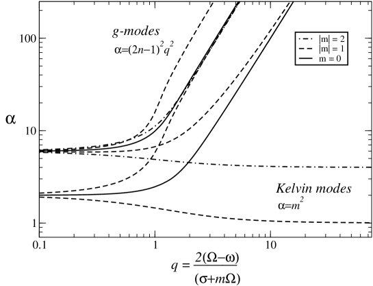
Figure 1: An illustration of the relation between the numerically determined angular eigenvalues $\alpha$ and the spin parameter $q$. The eigenvalues for the g-modes asymptote to $\alpha\approx(2n-1)^{2}q^{2}$ for $n=1,2,3...$ while the trapped Kelvin modes correspond to $\alpha\approx m^{2}$ for large $q$.

Having defined the angular eigenvalue $\alpha$, we obtain the two equations

$$-\xi^{r\prime}_{\mathrm{o}}-\left\{\left(1-{2M\over r}\right)^{-1/2}{p_{1}\over\Gamma_{1}p}-\left[\left(1-{2M\over r}\right)^{-1/2}{\rho g\over\Gamma_{1}p}-{2\over r}\right]\xi^{r}_{\mathrm{o}}\right\}=-\left(1-{2M\over r}\right)^{-1/2}{\alpha p_{1}\over\rho(\sigma+m\Omega)^{2}r^{2}}$$ (62)

and

$$\rho\left[\left(1-{2M\over r}\right)^{-3/2}(\sigma+m\Omega)^{2}+\left(1-{2M\over r}\right)^{-1/2}g\mathcal{A}\right]\xi^{r}_{\mathrm{o}}=p_{1}^{\prime}\left(1-{2M\over r}\right)^{-1/2}{\rho g\over\Gamma_{1}p}p_{1}.$$ (63)

These equations simplify considerably if we introduce new variables $\eta=r^{2}\psi\xi^{r}$ and $\phi=p_{1}/\psi$, where

$$\psi=\exp\left[-\int\left(1-{2M\over r}\right)^{-1/2}{g\over c_{s}^{2}}dr\right]$$ (64)

and the “sound speed” follows from

$$c_{s}^{2}={p\Gamma_{1}\over\rho}$$ (65)

In terms of these new variables we get

$$-\eta^{\prime}=\left(1-{2M\over r}\right)^{-1/2}\left[{1\over\Gamma_{1}p}-\left(1-{2M\over r}\right){\alpha\over(\sigma+m\Omega)^{2}r^{2}\rho}\right]r^{2}\phi\psi^{2}$$ (66)

and

$$\phi^{\prime}=\left(1-{2M\over r}\right)^{-1/2}\left[(\sigma+m\Omega)^{2}+\left(1-{2M\over r}\right)gA\right]\dfrac{\rho\eta}{r^{2}\psi^{2}}$$ (67)

If we now assume that the radial dependence of the perturbations is described by $\eta\sim\phi\sim\exp(ikr)$, where $k$ is the radial wavenumber, we readily arrive at the dispersion relation

$$k^{2}=\left(1-{2M\over r}\right)^{-1}\left[(\sigma+m\Omega)^{2}+\left(1-{2M\over r}\right)g\mathcal{A}\right]\left[{\rho\over\Gamma_{1}p}-\left(1-{2M\over r}\right){\alpha\over(\sigma+m\Omega)^{2}r^{2}}\right]$$ (68)

We now use the Brunt-Väisälä frequency $N^{2}=-g\mathcal{A}$ and an analogue to the standard Lamb frequency;

$$L^{2}_{\alpha}={\alpha c_{s}^{2}\over r^{2}}$$ (69)

Implementing a dimensionless corotating oscillation frequency

$$\kappa=\dfrac{\sigma+m\Omega}{\Omega}$$ (70)

we get the final result

$$k^{2}={\Omega^{2}\over c_{s}^{2}\kappa^{2}}\left(1-{2M\over r}\right)^{-1}\left[\kappa^{2}-\left(1-{2M\over r}\right)\left({N\over\Omega}\right)^{2}\right]\left[\kappa^{2}-\left(1-{2M\over r}\right)\left({L_{\alpha}\over\Omega}\right)^{2}\right].$$ (71)

In order to estimate the g-mode frequencies we recall that (cf. Bildsten, Ushomirsky and Cutler (1996); Townsend (2003))

$$\alpha\approx(2n-1)^{2}q^{2}=(2n-1)^{2}\left[{2(1-\omega/\Omega)\over\kappa}\right]^{2}\qquad n=1,2,3,...$$ (72)

for large $q$ (see Bildsten, Ushomirsky and Cutler (1996) for a discussion of the interpretation of the “quantum number” $n$). This behaviour is apparent in Figure 1. Expanding equation (72) for low frequencies (that is, for $\kappa<<N/\Omega$ and $\kappa<<L_{\alpha}/\Omega$) we find

$$\kappa\approx\sqrt{2}(2n-1)^{1/2}\left[1-{\omega\over\Omega}\right]^{1/2}\left(1-{2M\over r}\right)^{1/4}\left({N\over kr\Omega}\right)^{1/2}.$$ (73)

Even though this does not actually determine the mode-frequencies it allows us to estimate the magnitude of the relativistic effects. We see that there are two main effects: The obvious one is the gravitational redshift factor, which for a typical neutron star with $M/R\approx 1/5$ decreases the frequency by about 10% compared to the Newtonian case;

$$\left(1-{2M\over R}\right)^{1/4}\approx 1-{M\over 2R}\approx 0.9.$$ (74)

The rotational frame-dragging adds a further 10% to the decrease since

$$\omega\approx{2J\over R^{3}}={2I\Omega\over R^{3}}\approx{4M\Omega\over 5R}\quad\longrightarrow\quad\left[1-{\omega\over\Omega}\right]^{1/2}\approx 0.9.$$ (75)

Thus, we would expect the relativistic ocean g-modes to have frequencies roughly 20% lower than their Newtonian counterparts.

It is easy to argue that these relativistic corrections must be included if one wants to draw the correct conclusions from observed oscillations. For example, comparing our relativistic result to the corresponding Newtonian one (where $\omega$ and $M/R$ are both taken to be zero in (73)) we see that already for $n>2$ would we get $\kappa_{\mathrm{GR}}(n+1)<\kappa_{\mathrm{Newton}}(n)$. This means that the Newtonian formula would predict that the wrong mode was observed. This could be crucial if the aim is to study the inverse problem to put constraints on the physics of neutron star oceans.

As is clear from Figure 1 there is a distinct class of angular eigenvalues which do not exhibit the scaling discussed above. These solutions correspond to trapped Kelvin waves, and Townsend (2003) has shown that for large $q$ one gets

$$\alpha=m^{2}\dfrac{2mq}{2mq+1}\approx m^{2}$$ (76)

Following the same procedure as for the g-modes, we now find that

$$\kappa\approx m\left(1-\dfrac{2M}{R}\right)^{1/2}\dfrac{N}{\Omega kr}.$$ (77)

The derivation of this relation is valid as long as the radial wavenumber $k$ is taken to be large, i.e. for short-wavelength waves. Otherwise we would not have $\kappa<<N/\Omega$ and $\kappa<<L_{\alpha}/\Omega$. Now comparing to the Newtonian result (Townsend, 2003) one finds that the redshift reduces the frequency by about 20%, since

$$\left(1-\dfrac{2M}{R}\right)^{1/2}\approx 1-\dfrac{M}{R}\approx 0.8\ .$$ (78)

compared to the Newtonian case.

6 Ocean inertial modes: the r-modes

Given the relativistic version of the equations of motion it is interesting to ask whether we can estimate the frequencies of r-modes in the ocean. As discussed by eg. Townsend (2003) the r-modes are not well represented by the traditional approximation. However, it is straightforward to follow Provost, Berthomieu and Rocca (1981) and assume that the following scalings apply (see also Lockitch, Friedman and Andersson (2003)):

$$W \sim \sigma\Omega\sim\Omega^{3},$$

$$H_{1} \sim H_{2}\sim\sigma\sim\Omega,$$

$$p_{1} \sim \rho_{1}\sim\Omega^{2},$$

The relativistic continuity equation then immediately reduces to

$${\partial\over\partial\theta}(\sin\theta H_{1})+im\sin\theta H_{2}=0,$$ (79)

and a second equation relating $H_{1}$ and $H_{2}$ can be obtained by combining the $\theta$- and $\varphi$-momentum equations. This leads to

$$2i(\sigma+2m\Omega-m\omega)\sin\theta\cos\theta H_{2}+i(\sigma+m\Omega)\sin^{2}\theta{\partial H_{2}\over\partial\theta}+$$

$$[m(\sigma+m\Omega)+2(\Omega-\omega)(\cos^{2}\theta-\sin^{2}\theta)]H_{1}+2(\Omega-\omega)\sin\theta\cos\theta{\partial H_{1}\over\partial\theta}=0.$$ (80)

After some straightforward algebraic manipulations one can show that these two equations will be satisfied if

$$H_{1}={1\over\sin\theta}P_{lm}(\cos\theta)$$ (81)

and

$$\sigma=-m\Omega+{2m(\Omega-\omega)\over l(l+1)}.$$ (82)

It should, of course, be noted that this derivation only works as long we can take the frame-dragging, $\omega$, to be a constant, i.e. for oscillations in a thin shell. Anyway, we conclude that the frequencies of the ocean r-modes are sensitive to the surface value of the frame-dragging. The size of the effect can be appreciated if we take the ratio between the relativistic co-rotating frequency $\kappa_{\mathrm{GR}}$ and its Newtonian counterpart $\kappa_{\mathrm{Newton}}$. This immediately leads to

$${\kappa_{\mathrm{GR}}\over\kappa_{\mathrm{Newton}}}=1-{\omega\over\Omega}\approx 1-{4M\over 5R}\approx 0.84$$ (83)

Thus, the relativistic frame-dragging lowers the r-mode frequencies (in the rotating frame) by about 15%. This is in accordance with the results of e.g. Lockitch, Friedman and Andersson (2003) and Abramowicz, Rezzolla and Yoshida (2000).

Finally, it is worth pointing out that the calculation of general inertial modes is much more involved since one must account for the coupling of many spherical harmonics, see Lockitch, Friedman and Andersson (2003) for a recent discussion. In particular, such a calculation may be needed for the fastest spinning neutron stars since the g-modes will also be dominated by the Coriolis force when $\Omega>>N$.

7 Concluding remarks

We have shown how the so-called traditional approximation can be generalised to general relativity. This leads to a set of equations that ought to prove valuable for future studies of waves in the oceans of rotating neutron stars. The derivation of these equations required several assumptions in addition to those made in the Newtonian case. First of all, we have to make use of the Cowling approximation. That is, we neglect all metric perturbations. This may seem a drastic simplification, but it is a reasonable approximation for waves in the relatively low-density neutron star ocean. After all, such waves are not expected to lead to appreciable gravitational-wave emission. Secondly, we have to assume that the frame-dragging $\tilde{\omega}$ is constant, which restricts us to consider thin shells. Again, this should be a good approximation for neutron star oceans. Finally, and perhaps most interestingly, we have to neglect some terms of post-Newtonian order from the perturbed relativistic Euler equations, an approximation which is valid for low-frequency oscillations. Having made these various assumptions we can separate the eigenfunctions into a radial and an angular part. The angular eigenvalue problem is formally identical to the Newtonian one: it corresponds to solving Laplace’s tidal equation, which now depends also on the dragging of inertial frames. It should be emphasised that, since the two problems are identical we can use the results for the Newtonian angular problem also in the general relativistic case.

Our calculation prepares the ground for detailed calculations based on sophisticated models of the neutron star ocean. Given the eigenvalues to Laplace’s tidal equation, we need to solve the two radial differential equations (53) and (54), together with the relevant boundary conditions. Once one provides a description of the physics of the ocean, the solution of these equations should be straightforward. Here we opted to discuss the effect that general relativity has on various classes of ocean modes in a less quantitative way. We simplified our equations to the conditions that should prevail near the surface of a neutron star. This allowed us to derive a dispersion relation which we used to deduce to what extent the various classes of modes are affected by the gravitational redshift and the rotational frame-dragging. Thus we have shown that the mode frequencies are typically lowered by roughly 20%. This is not particularly surprising, but it should be noted that the overall effect is due to different combinations of the frame-dragging and the redshift factors for the different kinds of modes. We also discussed (briefly) the effect that general relativity has on the ocean r-modes.

Our estimates provide a strong argument in favour of using the derived formulae in more detailed (numerical) studies. In particular, we believe it is clear that one must account for the relativistic effects if the aim is to identify the individual ocean modes present in observed data.

References

- Abramowicz, Rezzolla and Yoshida (2000) Abramowicz, M.A., Rezzolla, L., Yoshida, S., 2000, Class. Quantum, Grav 19, 191
- Bildsten and Cutler (1995) Bildsten, L., Cutler, C., 1995, Astrophys. J., 449, 800
- Bildsten, Ushomirsky and Cutler (1996) Bildsten, L., Ushomirsky, G., Cutler, C., 1996, Astrophys. J., 460, 827
- Hartle (1967) Hartle, J., 1967, Astrophys. J., 150, 1005
- Heyl (2001) Heyl, J.S., preprint astro-ph/0108450
- Ipser and Lindblom (1992) Ipser, J., Lindblom L., 1992, Astrophys. J., 389, 392
- Lee and Saio (1997) Lee, U., and Saio, H., 1997, Astrophys. J., 491, 839
- Lockitch, Friedman and Andersson (2003) Lockitch, K.H., Friedman, J.L., Andersson, N., 2003, to appear in Phys. Rev D, preprint gr-qc/0210102
- Miles (1977) Miles, J., 1977, Proc. R. Soc. London, 353, 377
- Müller, Kelly and O’ Brien (1993) Müller, D., Kelly, B.G., O’ Brien, J.J., 1993, Phys. Rev. Let., 73, 11
- Provost, Berthomieu and Rocca (1981) Provost, J., Berthomieu, G., Rocca, A., 1981, Astron. Astrophys., 94, 126
- Strohmayer and Bildsten (2003) Strohmayer, T.E., Bildsten, L., New Views of Thermonuclear Bursts to appear in Compact Stellar X-Ray Sources, eds. W.H.G. Lewin and M. van der Klis, Cambridge University Press, preprint astro-ph/0301544
- Townsend (2003) Townsend, R.H.D, 2003, MNRAS, 340, 1020