Possibility of Magnetic Mass Detection by the Next Generation of Microlensing Experiments

Abstract

We study the possibility of magnetic mass detection by the gravitational microlensing technique. Recently the theoretical effect of magnetic mass in the NUT space on the microlensing light curve has been studied. It was shown that in the low photometric signal to noise and sampling rate of MACHO experiment light curves, no signature of NUT factor has been found. In order to increase the sensitivity of magnetic mass detection, we propose a systematic search for microlensing events, using the currently running alert systems and complementary telescopes for monitoring the Large Magellanic Clouds stars. In this strategy of observation, we obtain the magnetic mass detection efficiency and also the lowest observable limit of the NUT factor. This method of survey for gravitational microlensing detection can also be used as a tool for searching other exotic space-times.

1 Introduction

The gravitational microlensing method for detecting MAssive Compact Halo Objects (MACHOs) in the Milky Way halo has been proposed by Paczyński (1986). Many groups have contributed to this experiment and have detected hundreds of microlensing candidates in the direction of the galactic bulge, spiral arms and Large and Small Magellanic Clouds (LMC & SMC). Due to the low probability of the microlensing detection, less than 20 events have been observed by the EROS and MACHO groups in the direction of the Magellanic clouds (Lasserre et al. 2000; Alcock et al. 2000). The low statistics not only causes ambiguities in identifying the galactic model of the Milky Way, but also in some cases the microlensing results are at variance with the results of other observations (Gates and Gyuk 2001).
Comparing LMC microlensing events with the theoretical galactic models can give us the mean mass of MACHOs and the fraction of halo mass in the form of MACHOs. In the case that we use a Dirac Delta mass function for the MACHOs, the mass of MACHOs in standard halo model is obtained about $\sim 0.5M_{\sun}$. This means that the initial mass function of MACHO progenitors in the galactic halo should be different from that of the disk, because we neither see the low mass stars which should still exist nor heavier stars that would have exploded in the form of supernova (Adams & Laughlin 1996; Chabrier, Segretain & Mera 1996). Another contradiction is that if there were as many white dwarfs in the halo, as suggested by the microlensing experiments, they would increase the abundance of heavy metals via Type I Supernova explosions (Canal., Isern $\&$ Ruiz-Lapuente 1997). Also, recently Green & Jedamzik (2002) and Rahvar (2004) showed that the observed distribution of duration of microlensing events is not compatible with what is expected from the standard and non-standard halo models. They showed that the observed distribution is significantly narrower compared to what is expected from the galactic models.
The mentioned problems can be a motivation for establishing the next generation of the microlensing experiments. The new surveys will have the potential to increase the number of microlensing candidates and reduce the ambiguities due to Poisson statistics. The other improvements of the new surveys can be the higher sampling rates and the higher precision photometry of the light curves. More precise light curves will enable us to distinguish the deviations between the standard and non-standard light curves due to parallax or source finite-size effects (Rahvar et al. 2003). In the so-called non-standard microlensing candidates the degeneracy partially can be broken between the lens parameters, such as the distance and the mass of a lens. A better determination of the distance and the mass distributions of the lenses can help us to better identify the Milky Way halo model (Evans 1994).
Although the mentioned effects are in the background of a Schwarzschild space, it is also be possible that a MACHO which plays the role of the lens, resides in an exotic space-time such as the Kerr or the NUT space. Deviation of the space-time from the Schwarzschild metric causes deviation of the microlensing light curve from the standard one. Thus, studying the microlensing light curves not only can be used to determine the dark matter in the form of MACHOs but also as a unique tool to explore the other exotic space-times as well.
In the paper by Nouri-Zonoz and Lynden-Bell (1997) the gravitational lensing effect on the light rays passing by a NUT hole has been considered, using the fact that all the geodesics in the NUT space, including the null ones, lie on cones. The extension of this work to the microlensing light curve in the NUT space has been studied by Rahvar and Nouri-Zonoz (2003) and the possible existence of magnetic mass on the light curves of the MACHO group microlensing candidates has been tested. According to the analysis of the light curves, no magnetic mass effect has been found. Although the result showed that the effect of the NUT factor is almost negligible, one can not rule out the existence of NUT charge on that basis. The next generation of microlensing experiments may prove the (non-) existence of magnetic mass through a more careful study of the microlensing light curves.
Here in this work we simulate the microlensing light curves in the NUT metric according to a strategy for the next generation of microlensing surveys. The aim of this work is to obtain the observational efficiency for the magnetic mass detection and to find the lowest limit for the NUT charge that can be observed. Large Magellanic Cloud (LMC) stars are chosen as the target stars for monitoring. The advantage of using LMC stars as compared to the spiral arms and the galactic bulge stars is the lower contamination by blending and source finite-size effects, which can affect the NUT light curves. The other advantage of LMC monitoring is that it enables us to increase the microlensing statistics to put a better limit on the mass of the lenses and the mass fraction of the galactic halo in form of MACHOs.
The outline of this paper is as follows. In Section 2, we give a brief account on the microlensing light curve in the NUT metric and compare it with the Schwarzschild case. In Section 3, we introduce the observational strategy and perform a Monte-Carlo simulation to generate the microlensing light curves. Section 4 contains the fitting process to the simulated light curves to obtain the observational efficiency of the magnetic mass detection. The results are discussed in Section 5.

2 Gravitational microlensing in Schwarzschild and NUT metrics

The gravitational lensing effect occurs when the impact parameter of a lens with respect to the un-deflected observer-source line of sight is small enough that the deviation of source shape becomes detectable. In the case that of a point like source, the deflection angle is too small to be resolved by the present telescopes. This type of gravitational lensing which amplifies the brightness of the background star is called the gravitational microlensing. In the Schwarzschild metric the magnification is given by (Paczyński 1986):

$$A(t)=\frac{u(t)^{2}+2}{u(t)\sqrt{u(t)^{2}+4}},$$ (1)

where $u(t)=\sqrt{u_{0}^{2}+(\frac{t-t_{0}}{t_{E}})^{2}}$ is the impact parameter (position of the source in deflector plane normalized by the Einstein radius, $R_{E}$) and in which $t_{E}$ is the Einstein crossing time (duration of event) defined by $t_{E}=R_{E}/v_{t}$, where $v_{t}$ is the transverse velocity of deflector with respect to the line of sight. The Einstein radius is given by $R_{E}^{2}=\frac{4GMD}{c^{2}}$, where M is the mass of the deflector and $D=\frac{D_{l}D_{ls}}{D_{s}}$. $D_{l}$, $D_{l}s$ and $D_{s}$ are the observer-lens, lens-source and observer-source distances, respectively. The only physical parameter that can be obtained from a light curve is the duration of the event which is a function of the lens parameters such as mass, the distance of lens from the observer and the relative transverse velocity of the lens with respect to our line of sight.
In the case of gravitational microlensing, the configuration of the lens changes within the time scales of dozen of days while in the cosmological scales the lensing configuration is almost static. Since the magnification factor depends on the space-time metric, the gravitational microlensing technique may also be a useful tool to explore the other exotic metrics like the NUT space. In the NUT space the magnification due to the microlensing depends in addition, to an extra factor (magnetic mass) compared to the Schwarzschild space. It should be mentioned that the NUT space reduces to the Schwarzschild one when the magnetic mass ’${\it l}$’ is zero. So we expect that the microlensing amplification reduces to Equation (1) for zero magnetic mass. Rahvar and Nouri-Zonoz (2003) obtained the magnification in this space-time as follows:

$$A(u)=\frac{2+u^{2}}{u\sqrt{4+u^{2}}}+\frac{8R^{4}(2+u^{2})}{u^{3}(4+u^{2})^{3/2}}+{\mathcal{O}}(R^{8})+...,$$ (2)

where $R_{NUT}=\sqrt{2lD}$ is defined as the NUT radius (analogous to the Einstein radius) and $l$ is the magnetic mass of the lens. Parameter $R$ in Equation (2) is defined by dividing NUT radius to the Einstein radius, $R=R_{NUT}/R_{E}$. It is seen that in the NUT space the magnification factor, like the in the Schwarzschild case, is symmetric with respect to time. The extra second term implies a bigger relative maximum of the magnification factor for a given minimum impact parameter. we have also a shape deviation of the light curve with respect to the case of Schwarzschild metric.
The detectability of the NUT factor through studying microlensing, depends on the light curves quality (i.e. sampling rate and photometric error bars). In the next section we introduce a new strategy for microlensing observations in order to improve the microlensing light curves, both from the point view of the sampling rate and the photometric precision.

3 Light curves simulation in the NUT space

The strategy of the observation is based on using a survey as an alert system for microlensing detection with a follow-up setup. EROS is one of the groups that used an alert system to trigger ongoing microlensing events. We simulate EROS like telescope with the same sampling rate, considering $70\%$ clear sky at La Silla during the observable seasons of the LMC. A follow-up telescope is considered to observe with one percent photometry precision and sampling rate of at least once per night those events, that have been triggered by the first telescope. Here our aim is to simulate microlensing light curves in the NUT space by using the observational strategy, mentioned above.
It should be noted that there are at least two other important effects which are called blending and source finite-size effects that can change the light curves in symmetric manner like the NUT factor. Those effects are important because they may dominant over the effect of the NUT factor in the light curves. So, before starting the simulation procedure we give a brief account on those effects and include them in generating microlensing light curves in the NUT space.
The blending effect is due to the mixing of a lensed star and its neighbors lights, which is given as:

$$F(t)=F_{b}+A(t)F_{s},$$ (3)

where $F(t)$ is the measured flux, $F_{s}$ is the lensed source, $F_{b}$ is from the vicinity of lensed source and $A(t)$ is the amplification (Wozniak and Paczynski 1997). This effect is described by the blending parameter which is defined as $b=\frac{F_{s}}{F_{s}+F_{b}}$ and the observed magnification factor can be written as

$$A_{obs}(t)=1+b(A(t)-1).$$ (4)

The second altering effect on a light curve in a NUT space is the source finite-size effect which is caused by the non-zero size of projected source star on the lens plane. In this case, different parts of the source star are amplified by different factors. The relevant parameter of this effect is the projected size of the source radius on the lens plane, normalized to the corresponding Einstein radius ($U=\frac{xR}{R_{E}}$), where $x=\frac{D_{l}}{D_{s}}$ is the ratio of lens and source distances from the observer and $R$ is the size of the source radius. In the case of close source-lens distance compared to the observer-source distance, this effect becomes important.
To find the best field of source stars, we compare possible fields of observation such as the galactic bulge, the spiral arms and the Magellanic clouds to find the least blending and source finite-size effects. In the direction of galactic bulge the blending effect is high, since the field of target stars is crowded, except for the clump giants (Popowski et al 2000). For the spiral arms stars the blending effect is less than towards the galactic bulge while the source finite-size effect due to the self-lensing by the spiral arms stars is considerable. For the Small Magellanic Cloud (SMC) according to the blending and parallax studies of long duration event (Palanque-Delabrouille et al 1998), it seems that SMC is quite elongated along our line of sight, with a depth varying from a few kpc (the tidal radius of the SMC is of the order of $4$ kpc) to as much as $20$ kpc. So it is seen that due to high blending and source finite-size effects, SMC is not suitable for searching gravito-magnetic parameters. It seems that LMC is the best choice for this study. The other advantage of using this field is increasing the microlensing statistics which can be used in dark matter studies of the galactic halo.
Here in our simulation, we use the distribution of the blending factor according to the reconstructed blending parameter that has been obtained by the best fit to the LMC microlensing events. For the source finite-size effects of LMC stars, which become important in the case of itself-lensing, first we compare relative self-lensing abundance as compared to the galactic halo lensing and then evaluate the finite-size effect of those events on the light curves.
Comparing the optical depth for the standard galactic halo model $\tau_{halo}=1.2^{+0.4}_{-0.3}\times 10^{-7}$ (Alcock et al. 2000) with the optical depth obtained by the LMC itself $\tau_{self-lensing}=[0.47-7.84]\times 10^{-8}$ (Gyuk, Dalal and Griest 2000), with the mean value of $2.4\times 10^{-8}$ shows that the expected microlensing events lensed by the halo MACHOs are about one order of magnitude more than the LMC’s. The optical depth value of LMC self-lensing can be confirmed by studying the parallax effect on the light curves. Rahvar et al. (2003) showed that for using the same observational strategy that is proposed here, if the self-lensing is dominant, very few lenses (only those which belong to the disk) will produce a detectable parallax effect.
In order to evaluate the source finite-size effect on the microlensing light curves of LMC we perform a Monte-Carlo simulation to produce the distribution of the relevant parameter $U$. We use the LMC model introduced by Gyuk, Dalal and Griest (2000) to see the matter distribution in our line of sight. The probability of a microlensing event by a lens at LMC at a given distance from us is

$$\frac{d\Gamma(x)}{dx}\propto\sqrt{x(1-x)}\rho(x),$$

where $\rho(x)$ is the matter density distribution of LMC.
The source stars at LMC are chosen according to their color-magnitude distribution. We use the mass-radius relation (Demircan and Kahraman 1990) to evaluate the radius of stars in our simulation. The radius of source stars are projected on the lens plane and normalized to the corresponding Einstein radius to obtain the distribution of $U$s for the LMC self-lensing events. The mean value of $U$ according to our simulation is about $10^{-3}$, which we applied to obtain the gravitational microlensing light curves. For an impact parameter as small as $u_{0}=0.01$, where the NUT factor becomes important, the maximum magnification difference of a standard light curve and that of obtained by considering source finite-size effect is about one percent. On one hand this difference is less than our photometric accuracy and on the other hand the optical depth due to self-lensing is one order of magnitude smaller as compared to the galactic halo. The conclusion is that the source finite-size effect is not important in our analysis.

3.1 Simulation of light curves

The aim of this section is to simulate the microlensing light curves according to the observational strategy that was described before. We use the theoretical light curves to fit the simulated ones and evaluate the magnetic mass parameter of the NUT metric. The final result in this procedure is the observational magnetic mass detection efficiency, which can be applied in different galactic models. To start simulating the light curves, we use a uniform random function to generate the lens parameters.
The standard microlensing light curve in the Schwarzschild metric depends on 4 parameters, namely the base flux, $u_{0}$ (minimum impact parameter), $t_{e}$ (duration of the event) and $t_{0}$ (the moment of minimum impact parameter or maximum magnification). Taking into account the magnetic mass needs an extra parameter, $R$. The relevant parameters in simulating the light curves are chosen in the following intervals: $u_{0}\in[0,1]$, $t_{0}\in[0,2yr],$$t_{E}\in[5,365]$ days and $R\in[0,0.5]$.
The base fluxes $F_{b}$ of the background stars in the direction of LMC are chosen according to the magnitude distribution in the EROS catalogs (Lasserre 2000). Since it was shown that the contribution of the blending effect is important in this study, we use the blending distribution that has been obtained from the observed LMC microlensing events in order to use them in generating the light curves (Alcock et al. 2000). The light curves are simulated by using the sampling rate of EROS which is about one observation per six nights in average and is variable during the seasons. The average relative photometric precision $\Delta F/F$ for a given flux $F$ (in ADU unit) is taken from the EROS phenomenological parametrization which has been found for a standard quality image Derue (1999). In simulating the light curves, every photometric measurement is randomly shifted according to a Gaussian distribution that reflects the photometric uncertainties. Since the photometric uncertainty depends on the apparent magnitude of the background stars, the error bars of light curves decrease by increasing the brightness of background source during the lensing, (see Fig. 1).

3.2 Simulation of a simple alert system

The next step is to simulate an alert system to trigger the ongoing events and the follow-up observation by the secondary telescope. According to one of the EROS alert algorithms, the events will be announced as soon as their light curves exhibit 4 consecutive flux measurements above 4 standard deviations from the base line Mansoux (1997). It is clear that only the most significant microlensing events are selected by this algorithm. We have in fact considered several trigger thresholds, from a loose criterion (3 consecutive measurements above $3\sigma$ from the base line) to the strict criterion that was finally used. Even using this strict criterion, in average one false alarm due to variable stars or instrumental artifacts is expected per true microlensing alert Glicenstein (2002). This false alarm rate will induce some lost follow-up time, but for very limited durations, as it is usually very fast to discard a non-microlensing event. Fig. 1 shows an example of microlensing light curve that has been simulated, using the specifications of the primary and the secondary follow-up telescopes.
The efficiency of the alert system depends on the parameters of the lenses. In order to obtain the trigger efficiency in terms of the physical parameters such as the duration of events and $R$, we integrate over the irrelevant parameters such as the minimum impact parameter and the time of maximum magnification. Equation (2) shows that NUT parameter increases the maximum magnification or in another word decreases the effective minimum impact factor. The result is more trigger rate of microlensing events for those that have larger $R$. This effect is shown in Fig. 2. It shows that the trigger efficiency is increased by the long duration of microlensing events, which reflects a bigger probability for the observation of long duration events as compared to short events.

4 Follow-up telescope and fitting process to the light curves

We use a Monte-Carlo simulation to generate a large number of microlensing events. At the first step the lens parameters are chosen and the light curve is generated according to the primary telescope specification. Using the trigger system, in the case that an event is alerted, the secondary telescope starts its measurements with high sampling rate and photometry precision of the ongoing microlensing event.
The second telescope is supposed to be a partially dedicated telescope which follows the measurements of alerted events. The telescope is assumed to have about one percent precision in photometry and perform the sampling of events through all the clear nights. According to the Meteorological statistics of the La Silla observatory about $70$ percent of nights per year are clear. A one-meter telescope could achieve this precision with a long exposure of about $30$ min.
After simulating a large number of events by this strategy, we use the NUT and Schwarzschild theoretical microlensing light curves to fit the simulated ones. The least square method is used to fit the theoretical light curves on the data. An example of the fitting routine is shown in Fig. 1. In the case of fitting data with the NUT curve, with $R<0.1$ we encounter the degeneracy problem of fitting. It means that for $R$ close to zero we may obtain from the fitting a non-zero reconstructed value for $R$. To distinguish between the microlensing light curves affected by NUT charge and the standard ones we use the following criterion denoted by $\Delta\chi^{2}$, to be more than two

$$\Delta\chi^{2}=\frac{\chi_{Sch}^{2}-\chi_{NUT}^{2}}{\chi_{NUT}^{2}/N_{d.o.f}}\frac{1}{\sqrt{2N_{d.o.f}}},$$ (5)

where indices of the $\chi^{2}$ correspond to the type of the metric and $N_{d.o.f}$ is the number of degree of freedom in the NUT fitting. As complementary criterion in addition to the mentioned one we use the signal to noise ratio of $R$ to be more than two. We obtain the magnetic mass detection efficiency of MACHOs by dividing the reconstructed parameters of those events that pass two mentioned criteria, to the generated events. Fig. 3 shows two dimensional efficiency of magnetic mass detection in terms of $R$ and the duration of events. The detection efficiency of magnetic mass has direct correlation with $R$ as well as to the duration of the events. It is more practical to have efficiencies in terms of duration of events and $R$ which are shown in Fig.4. It should be mentioned that the blending effect decreases the detection efficiency of magnetic mass, as shown in Fig.4.

5 Conclusion

In this work we proposed a new strategy for microlensing observation that not only can be used for searching MACHOs of the galactic halo through observing the LMC stars, but also it can be a useful tool to explore exotic space-times around compact objects such as the NUT metric. As a result of our Monte Carlo simulation, we obtained the detection efficiency for magnetic mass. The minimum value for $R$ that can be observed by this method is about $0.1$. In order to evaluate the amount of detectable magnetic mass l, we use the relation between the magnetic mass and $R$ (Rahvar and Nouri-Zonoz 2003):

$$R=c\sqrt{\frac{{\it l}}{2GM}}.$$ (6)

EROS and MACHO experiments results propose that the mean value of the mass of MACHOs is about $0.5M_{\odot}$ (Alcock et al. 2000; Lasserre et al. 2000). It is worth to mention that this result is obtained in the standard halo model where the mean mass of MACHOs depends on the model that is used for the Milky Way. Assuming standard model for the Milky Way halo, according to equation (6) the minimum observable magnetic mass ${\it l}$ is evaluated to be about $14$ m. Non-existence of magnetic mass signal in the microlensing light curves can also put an upper limit for the value l $<$ 14 m in the MACHOs of the Milky Way.

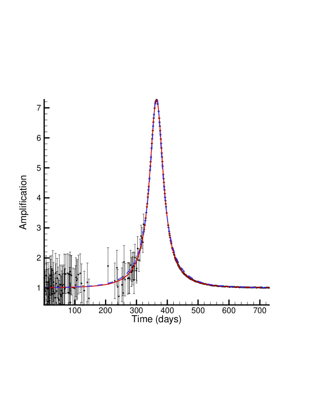
Figure 1: An example of the simulated light curves according to our proposed observational strategy for the next generation microlensing survey. The parameters of the light curve are chosen to be $t_{e}=100$ days, $t_{0}=365$ days, $u_{0}=0.3$, $b=0.88$ and $R=0.5$. The background star is chosen to have an apparent magnitude of 22. The dashed and solid lines show the result of least square fit of the the Schwarzschild and NUT theoretical light curves to the simulated data, respectively. The reconstructed NUT parameter derived from the fitting is $R_{rec}=0.501668$ with one sigma uncertainty of $0.001946$. $\chi^{2}/N_{dof}$ for this light curve from the NUT and the Schwarzschild fittings are 0.26 and 30.88.

Figure 2: The panels from up to down show the trigger efficiency in terms of the blending parameter, duration of events and $R$. The efficiency of the alert system depends on the blending parameter. This means that the bigger blending factor produce a lower maximum magnification. Also for the long duration events, there is a bigger chance to be alerted by the primary telescope. For the case of events with bigger $R$s, the peak of maximum magnification is elevated and the result is a bigger probability for those events to be alerted.

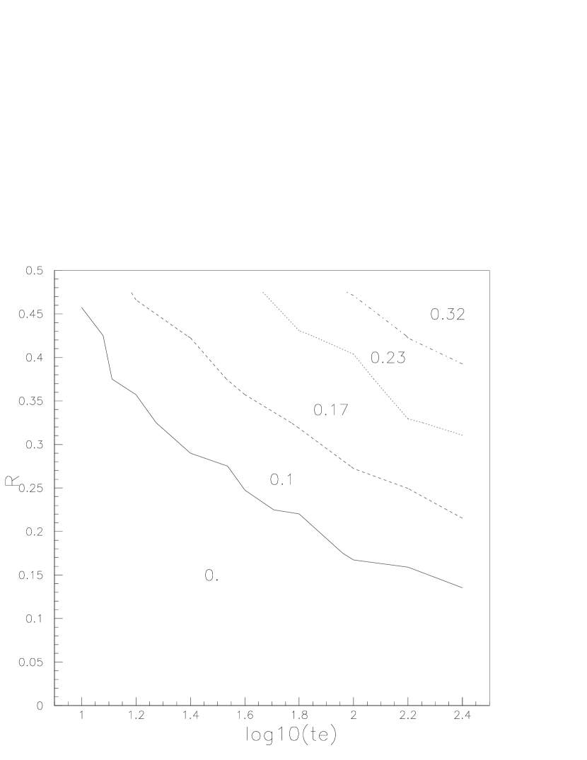
Figure 3: These contours show the two dimensional magnetic mass detection efficiency in terms of duration of events and $R$. The numbers between the contours show the amount of detection efficiency.

Figure 4: The panels from up to down show the magnetic mass detection efficiency in terms of blending parameter, duration of events and $R$. According to the first panel, the magnetic mass effect can be dominated by the blending. The detection efficiency has also direct dependence on the duration of events and $R$. A rough value for the minimum $R$ that can be detected is about $R=0.1$.

References

- Adams and Laughlin (1996) Adams, F., Laughlin, G., 1996, APJ, 468, 586.
- Alcock et al. (2000) Alcock C. et al. (MACHO), 2000, APJ, 542, 281.
- Canal., Isern and Ruiz-Lapuente (1997) Canal, R., Isern, J., Ruiz-Lapuente, P., 1997, APJ, 488, L35.
- Chabrier., Segretain and Mera (1996) Chabrier, G., Segretain, L., Mera D., 1996, APJ, 468, L21.
- Derue (1999) Derue F., 1999a, Ph.D. thesis, CNRS/IN2P3, LAL99-14 report.
- Demircan., Kahraman (1990) Demircan O., Kahraman G., 1990, Ap&SS, 181, 313
- Evans (1994) Evans N. W., 1994, MNRAS, 267, 333.
- Gates and Gyuk (2001) Gates I. E., Gyuk G., 2001, APJ, 547, 786.
- Gyuk., Dalal and Griest (2000) Gyuk G., Dalal N. and Griest K., 2000, APJ, 535, 90.
- Glicenstein (2002) Glicenstein J-F., 2002, private communication.
- Green and Jedamzik (2002) Green A. M., Jedamzik K., 2002, A&A 395, 31.
- Paczyński (1986) Paczyński B., 1986, APJ 304, 1.
- pop (00) Popowski P. et al. (MACHO), 2000, AAS, 197th AAS Meeting, #04.17; Bulletin of the American Astronomical Society, Vol. 32, p.1391
- Lasserre (2000) Lasserre, T.,2000. PhD. thesis, CNRS/IN2P3, LAL-report 97-19.
- Lasserre et al. (2000) Lasserre, T. et al. (EROS), 2000, A&A 355, L39.
- Mansoux (1997) Mansoux B., 1997, Ph.D. thesis, /sc CNRS/IN2P3, LAL report 97–19.
- Nouri-Zonoz and Lynden-Bell (1997) Nouri-Zonoz M., Lynden-Bell D., 1997, MNRAS, 292, 714
- (18) Palanque-Delabrouille et al. (EROS), 1998, A&A, 332, 1
- rahvar (2003a) Rahvar S., Nouri-Zonoz M., 2003, MNRAS, 338, 926
- Rahvar (2003b) Rahvar S., Moniez M., Ansari R., Perdereau O., 2003, A&A, 412, 81
- Rahvar (2004) Rahvar S., 2004, MNRAS, 347, 213
- Woz (97) Wozniak P., Paczynski B., 1997, ApJ, 487, 55