ADEMIS: A Library of Evolutionary Models for Emission-Line Galaxies: I- Dustfree Models

Abstract

We present an extensive set of stellar population synthesis models, which self-consistently include the (optical–far-UV) continuum emission from stars as well as the resulting emission-line spectrum from photoionized gas surrounding massive stars during their main- sequence-life time. The models are presented as a compiled library, ademis, available electronically. ademis  contains the equivalent widths and the intensities of the lines [O II] $\lambda\lambda$3727, H$\beta$, [O III] $\lambda$5007, H$\alpha$, and [N II] $\lambda$6584, which were calculated assuming a metallicity of 0.2, 0.4, 1.0, and 1.5 $Z_{\odot}$ and a wide range of ionization parameters. We investigate the regime of continuous star formation, assuming a Salpeter initial mass function, whose upper mass limit is an input parameter. The calculated equivalent width models, which are function of the burst age, are compared with the Jansen et al. atlas of integrated spectra for nearby galaxies. We reproduce the observed properties of galaxies along the full Hubble sequence and suggest how the metallicity and age of such galaxies might be roughly estimated.

1 Introduction

The presence of emission lines is a conspicuous feature of optical spectra of any galaxy that is currently forming stars. The lines result from the reprocessing of the UV ionizing radiation from the most massive of the young stars. Therefore, emission lines carry imprints of both phases, the newly formed stars versus the ‘excited’ interstellar medium (ISM), in a single observable quantity, the integrated optical spectrum. It is for this reason that the modeling of the emission-line spectra occurring in star-forming galaxies must include the interaction between both phases (stars $+$ gas) in a self-consistent manner. Partly for this reason, this paper will emphasize the study of equivalent widths (EWs or $W_{\lambda}$). The optical stellar continuum underlying the emission lines consists of much more than just the stars that ionize the gas. Actually, in any evolved stellar population, the optical and red continua are dominated by red giants and low-mass main sequence stars. In order to model the observed continuum properly, one must therefore consider the past stellar formation history of the whole stellar population, an essential step if the emission-line equivalent widths are to be calculated reliably.

Working toward these goals, García Vargas, Bressan & Díaz (1995), Stasińska & Leitherer 1996, Stasińska, Schaerer & Leitherer (2001) built models in which the spectral energy distributions (SEDs) generated by stellar evolutionary synthesis codes were used as input to photoionization calculations of emission-line strengths. These models aimed mainly at constraining the ages and metallicities of isolated extragalactic H II regions that are characterized by the absence or weakness of an old stellar population, suggesting a present-day strongly enhanced star formation rate. In short, these earlier models followed the evolution of spectral properties of an instantaneous burst of star formation. Recently, Kewley et al. (2001), Zackrisson et al. (2001) and Moy, Rocca-Volmerange & Fioc (2001) introduced models in which the star formation rate is constant for a few megayears, without interruption. These were used to derive the properties of starburst galaxies.

In an attempt to include the forgotten dust phase, Magris (1993) combined the spectral evolution synthesis code of Bruzual & Charlot (1993) with the photoionization code mappings i (Binette, Dopita & Tuohy 1985). The particularity of these models is that they included the effects of dust on the line- and continuum-emission in a self-consistent manner. On the other hand, only the solar metallicity case was studied, since detailed non-solar metallicity tracks and stellar spectral libraries were not complete at that time.

Barbaro & Poggianti (1997) have presented a model that is used to calculate the emission lines of [O II] $\lambda\lambda$ 3727 and of the Balmer series along with photometric quantities. The purpose was to estimate the present day star formation rate in late type galaxies. In their model, the star formation rate and the chemical evolution of the stellar phase for each Hubble type have been derived from their own chemical evolution model, assuming, on the other hand, a fixed solar composition for the ionized gas.

Charlot & Longhetti (2001) computed the line and continuum emission from star-forming galaxies and presented a family of estimators of the star formation rate, the nebular oxygen abundance, and the optical depth of the dust, in galaxies, as a function of the available spectral information. Their model is generally successful in reproducing the observed properties of template galaxies of different types. Their analysis, however, did not include the modeling of equivalent widths that are particularly suitable for analyzing the interrelated properties of the stellar and nebular phases.

We have developed a model along similar lines, which calculates, for an arbitrary star formation rate, both the nebular emission-line spectrum of the H II regions associated to the newly born massive stars and the SED of the underlying stellar population. However, rather than discussing line ratios and stellar energy distributions separately, our work will emphasize the relationship between the two phenomena, by presenting our model results as a library, ademis, of emission-line equivalent widths. As supplementary information, the tables also include the line luminosities of the most prominent species observed in normal star-forming nearby galaxies, i.e. [O II] $\lambda\lambda$3727, H$\beta$, [O III] $\lambda$5007, H$\alpha$, and [N II] $\lambda$6584. The models are characterized by a metallicity range of 0.2, 0.4, 1, and 1.5 times solar (gas $+$ star) and consider rates of star formation that are constrained by both the line and the stellar continuum emission, of galaxies of all Hubble types.

The method used to derive our evolutionary models is presented in §2. A description of the results from ademis follows in §3 accompanied by a comparison of the models with the Jansen et al. (2000a,b; hereafter JFFC) atlas of nearby galaxies. The conclusions are summarized in §4. A more extensive version than the adjoining tables of ademis models is available on the Web.

2 Computational Method

The method used to derive the nebular synthetic spectrum consists first in obtaining the ionizing spectrum corresponding to the hot main -sequence stars of an arbitrary stellar population. This ionizing spectrum is subsequently used by a photoionization code to compute the emission-line spectrum. The line fluxes are then combined with the integrated continuum spectrum of the stellar component to provide us with the equivalent widths of the emission lines of interest.

2.1 The Population Synthesis Code

One of our aims is to derive a nebular spectrum fully consistent with the young stellar population from which arise H II regions within an evolved normal galaxy. Special care must therefore be given to the population synthesis of the star-forming regions. For this purpose, we use the latest version of the evolutionary population synthesis code of Bruzual & Charlot (2003, hereafter BC03).

With this code, we can derive the spectrophotometric properties of any specified stellar population. For a given star formation rate (SFR) and initial mass function (IMF), a model consists of a set of spectra of the integrated stellar population calculated at 221 different ages $t$. Each such spectrum is defined at a common set of wavelength points covering the range 5–100 $\mu$m. The BC03 code, furthermore, can store separately the contribution of stars in different evolutionary stages. In the current work, it was necessary to generate an integrated spectrum for all the stars and another one for the subpopulation of main-sequence (MS) stars only. This latter spectrum was essential to derive the ionizing SED, which excites the H II regions and whose contributors consist exclusively of massive MS stars. This procedure excludes, for instance, other types of hot stars that generate ionizing photons, such as planetary nebulae nuclei, white dwarfs, or core helium-burning stars, which are irrelevant to young H II regions. In a separate paper, we have verified that the small H$\alpha$ widths of normal ellipticals might be explained by photoionization from post-AGB stars alone (Binette et al. 1994).

The time-evolution of the stellar population is followed using the Girardi et al. (2000) stellar tracks for low- and intermediate-mass stars (i.e. from 0.15 to 7 M_⊙), which are the most recent set from the Padova group, and the Bertelli et al. (1994) tracks for stars from 9 to 120 M_⊙. The advantage of these models with respect to earlier ones is that the data-base is computed with a homogenous input physics for all stellar tracks in the grid. For instance, moderate convective overshooting from convective cores and mass loss from massive stars are taken into account. In the most recent version used here, these tracks have been improved further with the adoption of new low-temperature opacities (see Girardi et al. 2000 for details)

The Kurucz stellar atmospheres spectra library (distributed by Lejeune, Cuisinier, & Buser 1997) has been adopted to compute the stellar properties of stars with $T_{eff}<50,000$ K. For the higher temperature stars, in order to give an adequate treatment to the ionizing continuum of hot MS stars, we use the Rauch (1977) NLTE model atmospheres for $\lambda<2000$ Å, and a simple black body spectrum for larger wavelengths. We recognize that large differences exist in the ionizing flux between LTE model atmospheres that include only H, He, C, N, O, and Ne, (like the Hummer & Mihalas (1970) models used in the emission-line synthesis of Magris (1993)) and the NLTE Rauch (1997) models, which include the opacity of heavier elements from Li to Ca. Despite these differences, we find, however, that the general properties of the ionizing flux that emerges from MS stars in a composite stellar population are not significantly affected. The reason is that high-mass stars have a relatively short lifetime for $T_{eff}$ hotter than $50,000$ K, and their contribution to the integrated spectrum of a composite stellar population becomes insignificant for any lasting star formation burst.

2.2 The Photoionization Code

To compute the nebular spectrum, we use the multipurpose shock/photoionization code mappings ic described by Ferruit et al. (1997); see also Binette et al. 1985), in which the ionization and thermal structure of the nebula are computed in a standard fashion, assuming local ionization and thermal equilibria throughout the nebula. The calculation is made at a progression of depths in the nebula, until all the ionization radiation has been absorbed.

For the nebular gas distribution, we adopt a simple slab geometry as in the work of Shields (1974), who argued that the integrated line spectrum was not significantly different from that calculated with the more usual spherical geometry. It is also the geometry preferred for the Orion nebula as modeled by Baldwin et al. (1991) or Binette, Gonz lez-G mez & Mayya (2002). The rationale is that H II regions are rather chaotic in appearance, showing evidence of strong density fluctuations with much of the emission coming from condensations or ionized “skins” of condensations. The relation between the dimensionless ionization parameter $U$, as defined in this work, and the emission lines, is also more straightforward and intuitive in the plane-parallel slab case.

Our set of solar abundances is taken from Anders & Grevesse (1989). When varying metallicity, we will assume that the abundances scale with metallicity in a linear fashion for all elements except helium and nitrogen. The He/H ratio will be kept constant at the solar value. The observed behavior of the N/O ratio in local and external H II regions suggests that the nitrogen abundance increases via secondary nucleosynthesis for metallicities above 0.23 solar (van Zee, Salzer & Haynes 1998; see Henry and Worthey 1999 for a review). To represent such N/O behavior, we adopt the following relations (Dopita et al. 2000):

$$\log({\rm N/H})=-4.57+\log(Z_{gas}/Z_{\odot});~{}~{}~{}\log(Z_{gas}/Z_{\odot})\leq-0.63$$

$$\log({\rm N/H})=-3.94+2\log(Z_{gas}/Z_{\odot});~{}~{}~{}{\rm otherwise}$$

where $Z_{gas}$ denotes the gas phase metallicity.

2.3 The Jansen et al. atlas as comparison sample

We will compare the predictions of our model with the spectrophotometric atlas of nearby galaxies of JFFC, which is ideal for this purpose, since it includes a representative sample of galaxies spanning the whole Hubble sequence and extending to lower luminosity systems than the Kennicutt (1992) sample. This sample is frequently referred to as the Nearby Field Galaxy Survey (NFGS). Such a comparison with the JFFC data will allow us to test the global properties of our models in the observational framework of a wide range of galaxy luminosities. The full sample includes 196 nearby galaxies from E to Irr, of luminosities in the range $M_{B}=-14$ to $-22$. However, of the 141 objects with detected H$\alpha$ emission, we will consider only those galaxies for which the equivalent widths EW$(\hbox{H$\alpha$})>10$ Å and EW$(\hbox{H$\beta$})>5$ Å. This will ensure a reliable measurement of Balmer decrements according to Jansen, Franx, & Fabricant (2001) and leave us with a sample of 85 objects. The atlas contains the equivalent widths and line ratios with respect to H$\beta$ of the following lines: [O II] $\lambda\lambda$ 3727, H$\delta$, H$\beta$, [O III] $\lambda$4959, [O III] $\lambda$5007, He I $\lambda$5876, [O I] $\lambda$6300, [N II]$\ \lambda$6548, H$\alpha$, [N II]$\ \lambda$6584, [S II]$\ \lambda$6716, and [S II]$\ \lambda$6731.

Since Jansen et al. (2001) have reported that the Balmer emission-line fluxes and equivalent widths given in JFFC were only partially corrected for stellar absorption, we have applied the additional correction suggested by these authors of 1 and 1.5 Å (EW) for H$\beta$ and H$\alpha$, respectively.

We corrected all line ratios for interstellar reddening by comparing the observed Balmer decrement, H$\alpha$/H$\beta$, with the case B recombination value of 2.85 (appropriate for $n_{e}\approx 10^{2}-10^{4}cm^{-3}$ and $T=10^{4}$K; Osterbrock 1989), and using the Nandy et al. (1975) Galactic extinction curve as tabulated by Seaton (1979).

2.4 Grid of photoionization calculations

Photoionization models were calculated using the various ionizing SEDs computed by the BC03 code. These SEDs differ by the age $t$ of their stellar population and correspond to MS stars, which were all formed at $t=0$, following a simple Salpeter (1955) IMF that covers a mass range comprised between a lower and upper mass limit, $m_{low}$ and $m_{up}$, respectively. The adopted lower limit is $m_{low}=0.09$ M_⊙ in all models. Because of the crucial role played by the upper mass limit on the hardness of the energy distribution, we have explored a wide range of upper mass limits: $m_{up}=$ 120, 100, 90, 80, 70, 60, 50, and 40 M_⊙. As for the metallicity of the stellar population, $Z_{\ast}$, we have calculated solar metallicity models ($Z_{\ast}=0.019$) as well as metal-poor ($Z_{\ast}=0.008$ and 0.004) and metal-rich ($Z_{\ast}=0.03$) models.

2.4.1 Usefullness of the hardness parameter $\eta$

We measure the hardness of the ionizing spectrum using the ratio between the flux of stellar photons (quanta s^-1) emitted above 24.6 eV and those emitted above 13.6 eV, $\eta=Q_{He^{0}}/Q_{H^{0}}$. The hardness $\eta$ can be associated with the cluster equivalent effective temperature, frequently used by H II region modelers (e.g. Shields & Tinsley 1976; Stasińska 1980; Campbell 1988).

In Fig. 1a, we show the hardness, $\eta$, as a function of $m_{up}$, of various ionizing distributions that are later used in photoionization calculations. An instantaneous burst with a Salpeter IMF was assumed. Each curve corresponds to a different stellar track metallicity, $Z_{\ast}$, as labeled. The different curves show a reduction in $\eta$ with increasing metallicity, because the higher $Z_{\ast}$, the cooler the stellar evolutionary tracks, and therefore, the softer the SED (and the lower $\eta$). This behavior has previously been reported by McGaugh (1991), who used the zero-age point of the stellar evolution tracks of Maeder (1990) to compute the ionizing radiation field of a cluster of stars distributed as the Salpeter (1955) IMF. Even though the details about our respective ionizing spectra may differ, it is found in this work as in McGaugh, that for a given SED with a certain $\eta$, it is possible to encounter another SED with the same $\eta$ if we decrease (or increase) appropriately both $m_{up}$ and $Z_{\ast}$. This interesting property, inferred from instantaneous burst models, tells us that both parameters are in fact degenerate.

Figure 1b shows the temporal evolution of $\eta$ for a model with a continuous SFR calculated with a Salpeter (1955) IMF, $\hbox{$m_{up}$}\ =125\hbox{M${}_{\odot}$}$, and the metallicities as labeled. We can see that $\eta$ reaches a constant asymptotic value after $\approx 10^{7}$   yr, due to the equilibrium between the number of new born massive stars and the number of them evolving off the MS. The same kind of evolution occurs with any star formation rate provided it is continuous and either constant with time or monotonically decreasing. In Fig. 1b, we also show the behavior of $\eta(t)$ for the case of a solar metallicity instantaneous burst, for comparison (dashed line).

In our extensive grid of photoionization calculations, $U$ was varied over the wide range of $-4\leq{\rm log~{}}U\leq-1.5$ although, in practice, a more limited range suffices, as independently shown in the modeling of H II regions by different authors (e.g., Evans & Dopita 1985; Campbell 1988).

As for the nebular gas metallicity, $Z_{gas}$, as a rule we adopt the same value as for the stellar atmospheres, and we will thereafter use $Z$ to refer to the metallicity of either component.

As a result of these computations, we obtained an extensive grid of emission-line spectra parameterized according to $U$, $\eta$, and $Z$. We verified that it was sufficient to read the appropriate emission line fluxes from our grid of photoionization models, using $\eta$ as the lookup value. Models at intermediate values of the parameters $U$, $\eta$, and $Z$ are obtained by simple interpolation (in the log-plane) within the grid points. This procedure allowed us to do away with calculating separate new photoionization calculations each time $\eta$ changed.

2.4.2 Two standard diagnostic diagrams

In Figure 2 we show a standard diagnostic diagram of the relationship between
[O III]$\lambda 5007$/H$\beta$ and [O II]$\lambda\lambda 3727$/H$\beta$. The solid lines join discrete models (open circles) calculated by using the $m_{up}$ value that appears in panel b near the right extremity of each line. Different $m_{up}$-values correspond to different $\eta$-values with $\eta$ strongly dependent as well on metallicity as Figure 1 already showed. The dotted lines join points of constant $U$ (indicated as log $U$-values near the upper end of the curves). With a range of ionization parameter of about a factor of 10 ($-3.25<$ log $U<-2.25$) as plotted in this figure, and a range of metallicity between 0.4 and 1.5 $Z_{\odot}$, our photoionization calculations encompass the dispersion in the [O III]/H$\beta$ versus [O II]/H$\beta$ relation observed in the JFFC sample of galaxies.

The same range in ionization parameter and metallicity characterizes the extragalactic H II region sequence of Dopita et al. (2000). Similarly, Bresolin, Kennicutt & Garnett (1999), who used a different but scalable definition of $U$, applicable to their geometry, concluded that a range of only a factor of 10 in $U$ suffices to reproduce the optical emission-line spectrum of their sample of spiral galaxy H II regions. Our models also happen to overlay the correlation presented by Kobulnicky, Kennicutt, & Pizagno (1999) in their [O III]/H$\beta$ versus [O II]/H$\beta$ diagram, which superposes indifferently individual H II regions and galaxy integrated ratios.

In Figure 3 we show the line ratio diagnostic diagram of [O III]/[O II] versus [N II]/[O II], which Dopita et al. (2000) suggests as being optimal for separating variations in the ionization parameter from variations in chemical abundance. The upper panel has been calculated with a simple zero-age stellar population, while the lower panel used a $10^{7}$ y old population formed according to a continuous SFR prescription. The [O III]/[O II] ratio has been established to be useful for determining the ionization parameter (e.g. McGaugh 1991), while the [N II]/[O II] ratio was found to be virtually independent of the ionization parameter, albeit very sensitive to the abundance for metallicities above 0.23 solar. This Figure indicates that the galaxies in the JFFC sample span a range in abundances from 0.2 solar up to solar or possibly 1.5 times solar, without any evidence for much higher metallicity objects. As in Figure 2, log $U$ spans the range $-3.25$ to $-2.25$.

Interestingly, the continuous SRF models of Fig. 3b overlap better the observational points than the zero-age models of Fig. 3a. This simply results from having a softer SED (smaller $\eta$) in the continuous SFR case, which produces models with a lower [O III]/[O II] ratio.

2.4.3 The synthesis of line spectra, stellar spectra and EWs

The SED of a given stellar population with age $t$ and arbitrary SFR, IMF, and $Z$ is computed using the BC03 code. From there, the SED corresponding exclusively to MS ionizing stars is used to derive $\eta$ and $Q_{H^{0}}$, the number of ionizing photons, which then allows us to infer the nebular emission-line spectrum by simple interpolation within the grid of H II region models, as described in §2.4.1. Finally, each emission-line equivalent width $W_{{\lambda}_{i}}(t)$ of line $i$ at wavelength $\lambda_{i}$ corresponding to the above evolutionary age $t$ is derived by dividing the line luminosity $L_{i}^{l}(t)$ by the SED luminosity $\bar{L}^{\ast}(\lambda_{i},t)$ of the integrated stellar population (i.e. all stars included) averaged over a fixed narrow band-pass $\Delta_{\lambda_{i}}$.

2.4.4 The concept of “equivalent H II region”

In the present model, we are assuming that the integrated emission line spectrum of galaxies is well represented by an “equivalent H II region,” ionized by a cluster of MS stars with the same mass spectrum as the whole galaxy. In support of this assumption, it has been shown by Kobulnicky et al. (1999) that the integrated [O II] and [O III] line luminosity mimics that of individual H II regions, and that the chemical abundances of the gas phase derived from individual nebulae or from integrated galaxy spectra coincide at least within the intrinsic uncertainties of the proposed abundance determination method. For ages older than 10 Myr and for a continuous star formation rate, the number of newly born massive stars relative to those having aged and producing less ionizing photons, achieve a near steady state regime of constant hardness, as can be seen in the right-hand panel of Figure 1, which shows the time evolution of $\eta$ for different continuous SFR. In this adopted scenario, the shape of the ionizing spectrum depends therefore only on the IMF and the metallicity of the stellar population. We are implicitly assuming that the error introduced by calculating the nebular spectra using a unique (but variable) galaxy age $>10$ Myr (rather than taking into account a distribution of H II region ages), is small in comparison with the uncertainties introduced by the other nebular parameters. Actually, our models are intended for comparison with normal galaxies, which are massive enough to minimize the dispersion because of statistical fluctuations in the sampled population. However, as has been pointed out by Cerviño et al.  (2002), this question is susceptible to be investigated in more detail.

Interestingly, if one seeks the equivalent $m_{up}$ of a zero-age instantaneous burst (Fig. 1a), which would reproduce the same SED hardness $\eta$ as that from the corresponding asymptotic value in the continuous SFR case with $\hbox{$m_{up}$}=125\hbox{M${}_{\odot}$}$ (Fig 1b) and with the same $Z$, one finds that this zero-age equivalent $m_{up}$ is $\simeq 60\hbox{M${}_{\odot}$}$. This result was confirmed for all the metallicities studied in this paper. It follows that the continuous SFR models of Fig. 3b with $\hbox{$m_{up}$}=125\hbox{M${}_{\odot}$}$ are, to all practical purposes, equivalent to a zero-age instantaneous burst with $\hbox{$m_{up}$}\simeq 60\hbox{M${}_{\odot}$}$.

3 Model results and discussion

We first discuss the principal results of our model predictions based on exponentially declining SFRs and then proceed to compare these with the spectrophotometric atlas of JFFC.

3.1 An atlas of calculated equivalent widths for non-instantaneous bursts

Table 1 summarizes the contents of our model grid ademis. The models listed correspond to the Salpeter IMF, with $\hbox{$m_{up}$}=125\hbox{M${}_{\odot}$}$, and a SFR $\Psi(t)$ exponentially declining with time:

$$\begin{array}[]{c}\Psi(t)=\tau^{-1}{\rm exp}(-t/\tau)\;,\end{array}$$ (1)

with $\tau=5$, and 9 Gyr, as indicated. The gas and metallicity of the stellar population are the same in all models of Table 1, covering the two cases of $Z_{\ast}=Z_{gas}=Z=1$ as well as 0.4 $Z_{\odot}$. The ionization parameter is log $U=-3.00$. In the electronic version, the models cover a wider range of the following parameters: $\tau=1$, 3, 5, 7, and 9 Gyr, and $\infty$ (i. e. constant SFR), log $U=-3.25$, $-$3.00, $-$2.75, $-$2.50 and $-$2.25, $\hbox{$m_{up}$}=40$, 60, 80 and 125 M_⊙ and $Z=0.2$, 0.4, 1.0 and 1.5 $Z_{\odot}$ (§2.2).

In Table 1, column (1) gives the metallicity $Z$, column (2) $\tau$ (see eq. 1), column (3) $m_{up}$ (in units of M_⊙), column (4) ${\rm log}U$, column (5) the age $t$ of the burst (in units of years), column (6) the hardness of the ionizing MS spectrum $\eta$. In column (7), we list $Q_{H^{0}}$, the ionizing photon luminosity of MS stars (s^-1) per unit solar mass of the parent galaxy total mass. column (8) contains the absolute visual magnitude, $M_{V}$, per unit solar mass of the parent galaxy mass. In columns (9)-(13) we present the equivalent widths of [O II], H$\beta$, [O III], H$\alpha$, and [N II] (see §2.4.3). The emission-line fluxes of [O II], H$\beta$, [O III], H$\alpha$, and [N II], shown in columns (14)-(18), are in ergs s^-1 per unit solar mass of the parent galaxy mass.

3.2 Relationships between EWs and metallicity $Z$ or age $t$

The relationship between $W_{\lambda}$([O II]) and $W_{\lambda}$(H$\alpha$) as a function of time for an exponentially declining SFR (Eq. 1) with a fixed $\tau=3$ Gyr is shown in Fig 4. Each line joins models of increasing age $t$, from right to left, keeping the ionization parameter constant. The three curves in each inset correspond to different ionization parameters, covering the values: log $U$ = $-$2.75, $-$3.00 and $-$3.25 (long-dashed curve). Models for four different upper mass limits $m_{up}$ of 125, 80, 60 and 40 M_⊙, are depicted in the four panels of Figs. 4a–d, respectively. The model metallicity varies from inset to inset, in a vertical fashion, to cover the four cases $Z=0.2$ (highest inset), 0.4, 1.0, and 1.5 (lowest inset). As a reference, a star and a circle are used to indicate ages of 1 and 12 Gyr, respectively. Filled squares represent the JFFC sample (§2.3). The same models are shown in Figures 5a–5d ($m_{up}$) for the case of $W_{\lambda}$([O III]) versus $W_{\lambda}$(H$\alpha$), while for $W_{\lambda}$([N II]) versus $W_{\lambda}$([O II]), they appear in Figs. 6a–6d. In Figure 7, we plot $\hbox{$W_{\lambda}$}(\hbox{[{O~{}III}]})+\hbox{$W_{\lambda}$}(\hbox{[{O~{}II}]})$ versus $W_{\lambda}$(H$\alpha$), assuming the value $\hbox{$m_{up}$}\ =125\hbox{M${}_{\odot}$}$. We adopt a logarithmic scale in our figures since Jansen et al. (2000b) pointed out that their EWs plots show a near uniform dispersion when expressed in logarithmic units.

It is interesting to analyze Figs 4–7 in the light of the discussion of the data presented in §4.2 of Jansen et al. (2000b). We concluded the following:

1. Because high metallicity models appear too far below the data in Figs 4a–d when $\hbox{$m_{up}$}\lesssim 80\hbox{M${}_{\odot}$}$, we consider that our best case continuous SFR model favors high values for $m_{up}$. For the sake of the discussion, we will assume $\hbox{$m_{up}$}=125\hbox{M${}_{\odot}$}$ for the remainder of this Section and the next.

2. Although we cannot infer in a simple way the metallicity using EW diagrams, a comparison of models of different metallicities in Figure 4a and 5a tells us that galaxies with a high $W_{\lambda}$([O II]) and/or a high $W_{\lambda}$([O III]) (i.e. objects toward the upper right corner) could not be fitted satisfactorily using solar or above metallicity models. Therefore, our models suggest abundances lower than solar for this subset. This indication is consistent with the findings of Jansen et al. (2000b), who pointed out that these high $W_{\lambda}$([O II]) objects in fact correspond to a lower luminosity (and lower metallicity) subset of their survey.

3. The data show a trend of increasing $W_{\lambda}$([O II]) or $W_{\lambda}$([O III]) with $W_{\lambda}$(H$\alpha$). Our models suggest that these could in part be due to a younger age effect, since the solid lines present an angle of inclination that is comparable to the trend in the data. However, the increase in $W_{\lambda}$([O II]) or $W_{\lambda}$([O III]) [but not that of $W_{\lambda}$(H$\alpha$)] may be caused as well by a systematic trend in metallicity, since models shift vertically by large amounts when varying $Z$, as shown by the insets of Fig 4a. This is not surprising, given that the luminosities of collisionally excited lines are strongly dependent on the gas temperature, which, in turn, is mostly a function of gas metallicity. We conclude that variations in age $t$ and in metallicity $Z$ are the two most significant contributors to the trends seen in the data.

4. Even though a variation in the age $t$ of models mimics part of the trend observed in the data in Fig 4a, we cannot reliably estimate the age (or the metallicity) using $W_{\lambda}$([O II]). For instance, galaxies in the Jansen et al. (2000b) sample with $\hbox{$W_{\lambda}$}(\hbox{[{O~{}II}]})\gtrsim 30$Å are in general expected to possess subsolar abundances with $Z<0.5$ $Z_{\odot}$. [In that case, their observed $W_{\lambda}$(H$\alpha$) appears confined to values below $\sim 70$ Å.] However, much larger EW([O II]) than present in the current sample are in principle possible, but only if the H$\alpha$ equivalent widths were correspondingly very large. In our scheme, such an object would correspond to stellar bursts characterized by a very young stellar population. The predicted $W_{\lambda}$(H$\alpha$) in that case can be found amongst the models of Table 1.

5. In the case of the H$\alpha$ recombination line, as expected, its EW is independent of $U$, while (by definition) high- (low-) U models are characterized by higher (lower) [O III] EWs and lower (higher) [O II] EWs.

6. In models, $W_{\lambda}$([O III]) is much more sensitive to variations in $U$ (compare Fig. 5a with 4a) than $W_{\lambda}$([O II]). This is consistent with the range of values taken by $W_{\lambda}$([O III]) within the data, which are much larger than that of $W_{\lambda}$([O II]). We recall that the hardness $\eta$ becomes constant after an age as short as $\approx 10^{7}$   yr, as shown in §2.4.1, and therefore, changes in $W_{\lambda}$([O III]) are not due to changes in $\eta$, but are entirely due to changes in $Q_{H^{0}}$ and in the integrated stellar continuum level.

7. The [N II]–[O II] EW plot of Fig. 6 indicate that variations in age $t$ run almost vertically and are therefore nearly orthogonal with respect to variations in metallicity $Z$. Furthermore, the models are not sensitive to the ionization parameter. This EW diagram might therefore serve as an abundance diagnostic, a property worth investigating further.

8. The dependence on the ionization parameter is almost absent in the plot of $\hbox{$W_{\lambda}$}(\hbox{[{O~{}III}]})+\hbox{$W_{\lambda}$}(\hbox{[{O~{}II}]})$ against $W_{\lambda}$(H$\alpha$), as shown in Fig. 7.

3.3 The abundance–$m_{up}$ degeneracy

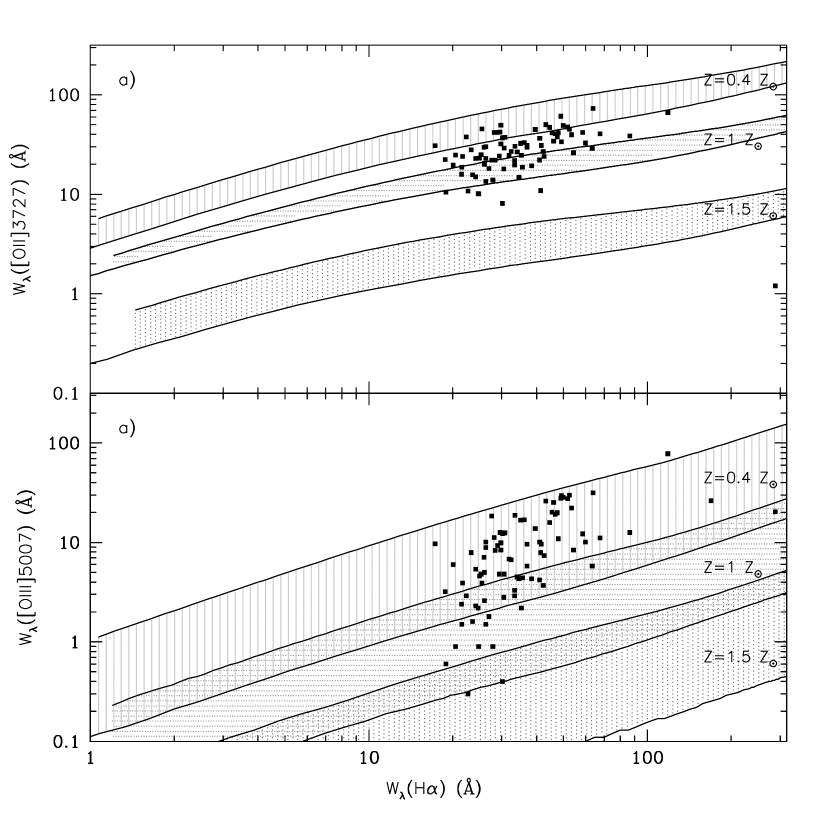
Figure 8: Relation between (a) $W_{\lambda}$([O II] $\lambda\lambda$ 3727) $vs.$ $W_{\lambda}$(H$\alpha$) and (b) $W_{\lambda}$([O III] $\lambda$ 5007) $vs.$ $W_{\lambda}$(H$\alpha$). Each shade corresponds to the loci of continuous SFR models with the same metallicity (as labeled), but with log $U$ comprised between $-3.25$ and $-2.50$, $\tau$ ranging between 1 Gyr, and $\infty$, and $m_{up}$ taking the values of 125, 80, and 60 M_⊙. The age $t$ increases from right to left. The three metallicities covered are $Z=0.4$, 1.0 and 1.5 $Z_{\odot}$. The values observed by JFFC are represented in each panel by filled squares.

In order to exemplify the degeneracy between abundance and $m_{up}$ (see Sec. 2.4.1) in the case of continuous star formation, we present in Figure 8 the loci occupied by models with metallicities 0.4, 1.0, and 1.5 times solar, in a plane defined by (panel a) $W_{\lambda}$([O II]) versus $W_{\lambda}$(H$\alpha$) and (panel b) $W_{\lambda}$([O III]) versus $W_{\lambda}$(H$\alpha$). Areas with different shades correspond to models with different $Z$-values (as labeled). The other parameters are log $U$ between $-3.25$, and $-2.50$, a SFR declining exponentially with time (Eq. 1) with $\tau$ anywhere between 1 Gyr, and $\infty$ (i.e. constant SFR), and a Salpeter IMF with $m_{up}$= 125, 80, and 60 M_⊙. These parameters encompass a wide range of possibilities for the galaxies considered. The main issue to highlight here is the extent to which metallicity and $m_{up}$ are degenerate as showed by the significant overlap between the different shaded areas in the [O III] and H$\alpha$ EW plot of Figure 8b. The abundance–$m_{up}$ degeneracy must therefore be taken into account for the analysis of emission line properties, especially in small [O III] equivalent widths galaxies, in order to determine the origin of the low excitation. Because of the low ionization potential of O to O⁺, [O II] does not suffer from such a degeneracy and it is therefore a better indicator of abundances in emission-line galaxies.

The comparison of our models with observed line ratios allows us to conclude that the metallicities of the galaxies in the JFFC sample do not extend beyond 1.5 $Z_{\odot}$and that an important fraction of them actually belongs to a galaxy population of lower metallicity than solar.

3.4 Varying the rate of SFR decline $\tau$

Models with different e-folding time $\tau$ (but equal $Z$ and $U$) show relationships between the [O II] or the [O III] EWs, and the H$\alpha$ EWs, very similar to those studied in §3.2, except for their temporal evolution rate, which scales differently. This is expected since the hardness of the ionizing SED is constant after $\approx 10^{7}$   yr, as shown in §2.4.1, and models of interest are typically much older than this. Also, since our EW models correspond to the properties of the whole host galaxy, the SED in the optical, against which the EW are defined, is not sensitive to the youngest star colors.

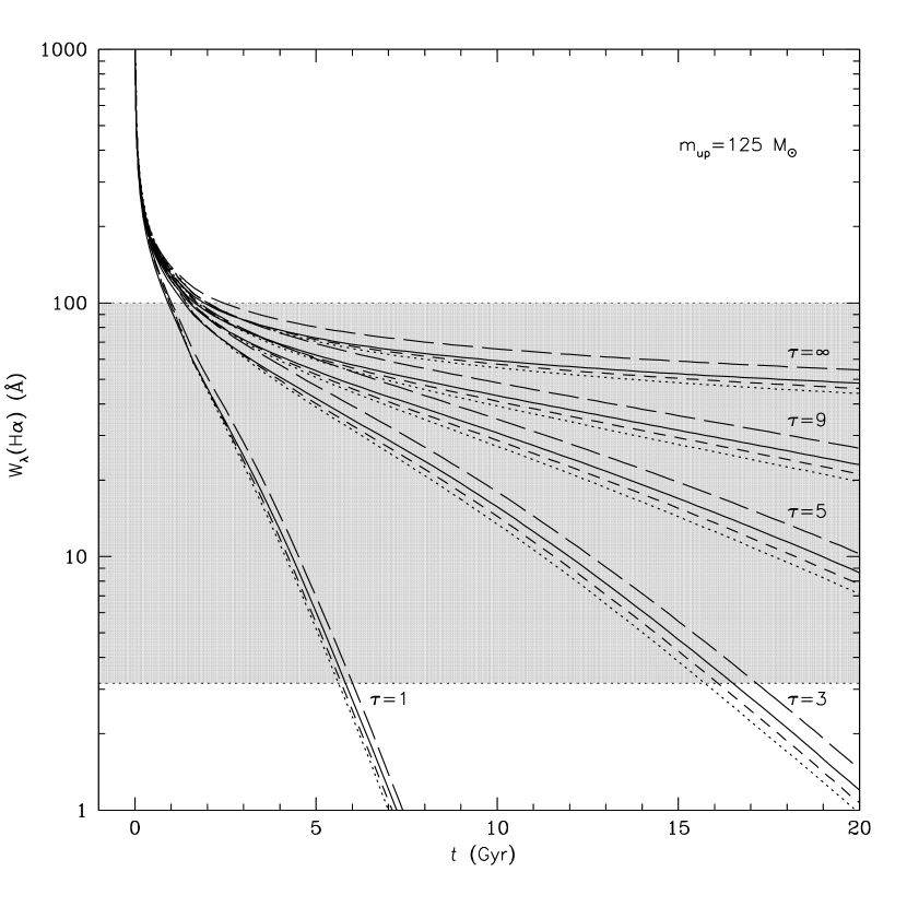
Figure 9: Evolution of $W_{\lambda}$(H$\alpha$) with age $t$ for models with a SFR declining exponentially with time, a Salpeter IMF, and $\hbox{$m_{up}$}=125\,\hbox{M${}_{\odot}$}$. The rate of SFR decline is represented by $\tau$, which takes on the values $\tau$ = 1, 3, 5, and 9 Gyr and $\infty$ (i.e. constant SFR), as labeled. The dotted line corresponds to models with $Z=0.2$ $Z_{\odot}$, the short dashed line to $Z=0.4$ $Z_{\odot}$, the solid line to $Z=1.0$ $Z_{\odot}$, and the long dashed line to $Z=1.5$ $Z_{\odot}$. The shaded area represents range of 97% of observed $W_{\lambda}$(H$\alpha$)-values from the JFFC sample of galaxies [three objects exceed the 100 Å bar, having a $W_{\lambda}$(H$\alpha$) of 169, 288 and 328 Å].

The equivalent width–age relationship, as expected and mentioned above, strongly depends on the adopted particular SFR history, as illustrated by Fig. 9, in which we plot the time evolution of $W_{\lambda}$(H$\alpha$) for similar models than shown in previous figures except that $\tau$ is now varied. We only consider the case $\hbox{$m_{up}$}=125\,\hbox{M${}_{\odot}$}$, which is the model favored by our discussion in §3.2. The horizontal lines circumscribe the region occupied by the JFFC galaxies. The $W_{\lambda}$(H$\alpha$) versus age relation is not sensitive to the ionization parameter. However, it shows a residual dependence on metallicity, as can be appreciated in Figure 9. This is simply due to variations in the mean effective temperature of the ionizing stars with $Z_{\ast}$, which brings about small changes in the number of ionizing photons and also to variations in the integrated stellar continuum.

The first conclusion reached from introspection of Fig. 9 is that even for the most active galaxies (in the sense of higher star-forming rates), the stellar population must be older than $\approx$ 1 Gyr in order to fit within the observed EW range. Actually, even allowing for a very long-lasting episode of high SFR, i.e. models with high $\tau$-values, the requirement that these models lie below the observed 100 Å $W_{\lambda}$(H$\alpha$) upper limit, imply such a lower limit on the burst age, as expected in a sample of normal field galaxies. On the other hand, we would conclude that galaxies from other samples, which would be observed to have $W_{\lambda}$(H$\alpha$) $>100$ Å, must therefore be actively forming stars, and their dominant stellar population could not be much older than 1 Gyr.

The second conclusion derived from Fig. 9 is that galaxies found with a small $W_{\lambda}$(H$\alpha$) ($\lesssim 10$Å) are currently forming stars at a very slow rate with respect to their previous SFR. This is implied by the requirement of a small $\tau$ ($\leq$ 3 Gyr) so that the models can reproduce $W_{\lambda}$(H$\alpha$) $\lesssim 10$ Å.

A more precise determination of the star formation history is not possible, using only $W_{\lambda}$(H$\alpha$). As is obvious in Fig. 9, the same $W_{\lambda}$(H$\alpha$) is obtained by either increasing or decreasing $t$ and $\tau$ simultaneously. The degeneration between both parameters can be overcome by using specific tracers. Kauffmann et al (2003), for instance, used the strength of the 4000 Å break as well as the stellar absorption line index H$\delta$ to constrain the star formation history of the galaxies. Recently, J. Mateu, G. Bruzual A., & G. Magris C. (2003, in preparation) have model-fitted the stellar continuum of the JFFC sample and were able to infer the temporal evolution of the SFR of the underlying stellar population for most of the sample.

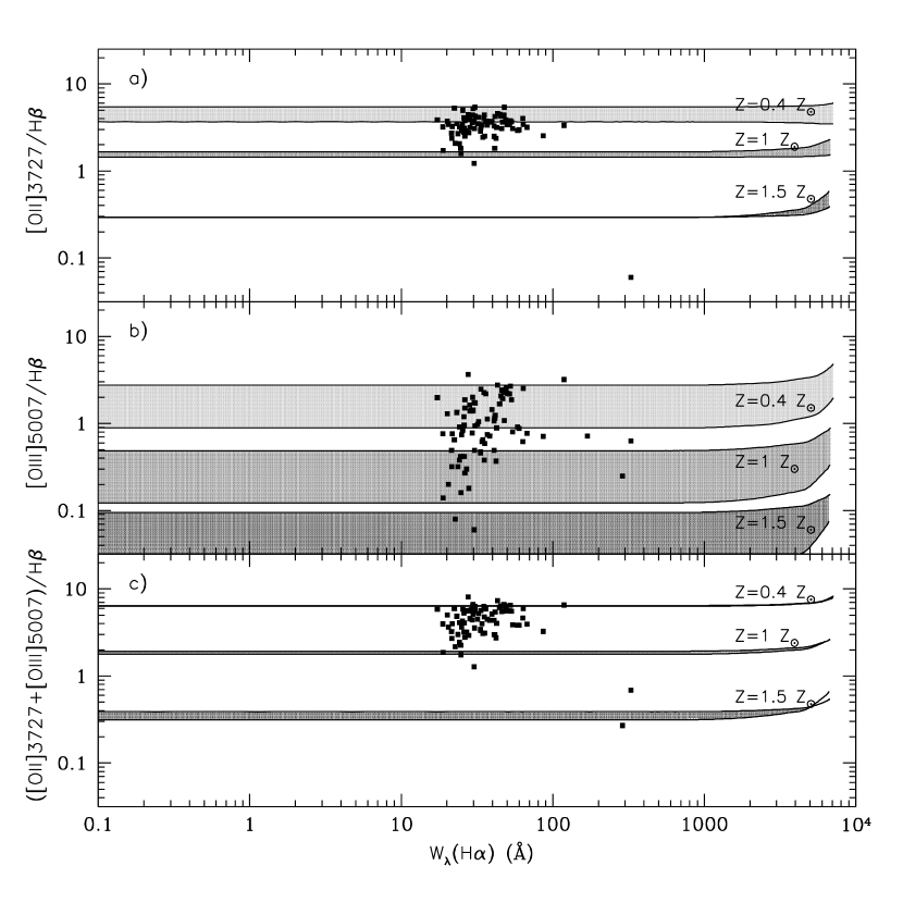
Figure 10: Relation between the line ratios (a) [O II]/H$\beta$, (b) [O III]/H$\beta$, (c) $(\hbox{[{O~{}II}]}+\hbox{[{O~{}III}]})/\hbox{H$\beta$}$, and the H$\alpha$ equivalent width. In each panel, strips with different shades correspond to models with a different metallicity $Z$, as labeled. Each shade indicates the loci of models with an exponentially declining SFR between $\tau=1$ Gyr and $\infty$. All models assume a Salpeter IMF and the same $\hbox{$m_{up}$}=125\hbox{M${}_{\odot}$}$. The relative thickness of each strip is mostly due to the dependence on the ionization parameter, which here spans the range $-3.25\leq{\rm log}~{}U\leq-2.50$. The age $t$ increases from right to left and can be read from Fig. 9 for any particular value of $\tau$. Filled squares represent the JFFC sample.

As for the line ratios [O II]/H$\beta$, [O III]/H$\beta$ and ([O II]$+$[O III]/)H$\beta$, their behavior as a function of the H$\alpha$ EW is shown in Figure 10 for models with a Salpeter IMF and $\hbox{$m_{up}$}=125\,\hbox{M${}_{\odot}$}$. Each strip represents the loci of models of the same metallicity with log $U$ anywhere between $-3.25$ and $-2.25$ and $\tau$ between 1.0 and infinity (equivalent to a constant SFR). The corresponding ages of the models can be inferred from Fig. 9. Since models with $Z=0.2$ and 0.4 would overlap, we only show the case $Z=0.4$. We infer from panel a that the [O II]/H$\beta$ ratio could give us a reasonable estimate of abundances, specially for metallicities above solar, while the classical abundance indicator ([O II]+[O III])/H$\beta$ ratio (Pagel et al. 1979), as expected, remains a better diagnostic since the shaded strips are much thinner in the corresponding panel c. The [O III]/H$\beta$ ratio in panel b, remains a poor estimator of metal abundance in the nebulae.

3.5 General discussion

Stasińska et al. (2001) presented instantaneous burst models for the evolution of H II galaxies and suggested that the presence of an underlying old stellar component was required to lower the $W_{\lambda}$(H$\beta$) predicted by their models sufficiently. Similarly, Moy et al. (2001) have shown that an instantaneous or a very short-lasting burst of star formation predicts very high hydrogen lines equivalent widths. Therefore, they added an underlying population to their starburst galaxy model. Our integrated continuous SFR model includes and evolves its own intrinsic older stellar population in a self-consistent manner. This has the effect of “raising” the continuum in the H$\beta$ and H$\alpha$ wavelength regions, thereby lowering the nebular emission line equivalent widths.

An important issue to emphasize is that the ademis model is able to simultaneously account for the observed oxygen-to-hydrogen emission-line ratios as well as for the H$\alpha$ equivalent widths. In any event, the presence of an older population affects EWs but not the line ratios. As has been explained in §2.4.1, in the case of a continuous SFR, the hardness of the ionizing spectrum evolves only during the first few Myr, until a balance between stellar births and deaths is established. In this latter regime, the parameters that govern the emission line ratios are the metallicity and the IMF upper mass limit, and, to a lesser extent, the slope of the initial mass function (a parameter not explored in this paper).

Even though our approach is not identical to that of Charlot & Longhetti (2001), both models have in common that they decouple the evolution of the ionizing stellar population from the evolution of the older stellar population since they require us to select, for a fixed metallicity, the hardness of ionizing spectrum. This is done in our case by appropriately selecting the most suitable IMF upper mass limit, or, in the case of Charlot & Longhetti, by selecting the stellar burst age.

4 Conclusions

We have presented a new library of models, ademis, which combine the stellar population history with the emission line-strengths. These models can be used to interpret the properties of objects that are characterized by either a very recent and strong burst or by a secular and lower star formation rate.

Starting from simple assumptions about the distribution of H II regions in disk galaxies, namely, a uniform distribution of dust-free gas and stars, in which young stars are distributed in mass in a similar fashion as the older stars, we have shown how it is possible to compute several properties of star forming galaxies. A photoionization code is used to compute the intensity of the emission lines, assuming no temporal evolution of $U$, while an evolutionary synthesis code provides the number luminosity and hardness of the MS ionizing photons. These, in conjunction with the photoionization code and the integrated stellar distribution, allow us to compute the temporal evolution of the emission line equivalent widths.

Diagnostic diagrams built by comparing pairs of equivalent widths of various lines, show that our model predictions fall in figures in the same region as the observed galaxies of JFFC. In particular, we conclude the following.

1. A factor of 10 in $U$ and a range in metallicity between 0.2 and 1.5 $Z_{\odot}$ seems appropriate to describe the observed properties of a representative sample of nearby galaxies.

2. The hardness of the ionizing continuum is constant after $10^{7}$ yr in case of a continuous SFR.

3. Our favored continuous SFR model with $\hbox{$m_{up}$}=125\hbox{M${}_{\odot}$}$ presents a hardness $\eta$ very similar to that produced by an instantaneous burst with an IMF having only $\hbox{$m_{up}$}=60\hbox{M${}_{\odot}$}$.

4. Galaxies with $\hbox{$W_{\lambda}$}(\hbox{[{O~{}II}]})\gtrsim 30$ Å and $W_{\lambda}$$(\hbox{H$\alpha$})\lesssim 70$ Å  appear to have subsolar abundances.

5. Galaxies with $\hbox{$W_{\lambda}$}(\hbox{H$\alpha$})\lesssim 100$ Å have a dominant underlying stellar population older than at least 1 Gyr. Only galaxies with a recent burst of star formation ($t\lesssim 1$ Gyr) are able to show H$\alpha$ EW in excess of 100 Å.

6. The information provided by the [O III] line is of limited use, owing to the strong $m_{up}$–$Z$ degeneracy, which complicates the interpretation of this high-excitation indicator, particularly in the case of low [O III] EWs.

Figure 1: (a) Behavior of $\eta$, the hardness of the ionizing continuum (as defined in §2.4.1), as a function of $m_{up}$, assuming an instantaneous burst with a Salpeter IMF and one of the following metallicities: $Z_{\ast}=0.2$, 0.4 , 1.0 and 1.5 $Z_{\odot}$. (b) Temporal evolution of the hardness for the same range in metallicity (as labeled) in the case of a continuous SFR decreasing exponentially with time, a Salpeter IMF and the same $m_{up}$ of 125 M_⊙. After 10 Myr, $\eta$ reaches an asymptotic value, which differs depending on metallicity, but can be shown to be independent, of the SFR provided that the SFR is continuous and either constant or monotonically decreasing. The dashed line corresponds to an instantaneous burst of solar metallicity with the same IMF and $m_{up}$.

Figure 2: Diagnostic plot of log ([O III]/H$\beta$) against log ([O II]/H$\beta$) for (a) $Z=0.2$ $Z_{\odot}$, (b) $Z=0.4$ $Z_{\odot}$, (c) $Z=1.0$ $Z_{\odot}$, and (d) $Z=1.5$ $Z_{\odot}$. The theoretical grid models were calculated with an ionizing spectrum from an instantaneous burst of age zero, a Salpeter IMF, and $\hbox{$m_{up}$}=125$, 100, 90, 80, 70 and 60 M_⊙, respectively. The models move up in the diagram with increasing $m_{up}$ [as labeled in panel (b)]. Solid lines join models (encircled dots) of equal $m_{up}$, i.e. constant hardness, while dotted lines join models of equal ionization parameter $U$. From left to right, log $U$ takes on the values of $-$2.25, $-$2.50, $-$2.75, $-$3.00, $-$3.25, respectively. Filled squares represent the observed reddening corrected ratios from the JFFC atlas (see §2.3). The arrow in (a) represents the dereddening vector corresponding to E(B–V) = 0.2.

Figure 3: Diagnostic plot of log([O III]/[O II]) against log ([N II]/[O II]) (a): for an instantaneous burst at zero age, and (b): for a continuous SFR at age 10 Myr, at which point the ionizing hardness $\eta$ has reached its asymptotic value (see Fig. 1b). In both panels, a Salpeter IMF with the same $\hbox{$m_{up}$}=125\hbox{M${}_{\odot}$}$ was assumed, and the nitrogen abundance was increased via secondary nucleosynthesis, as explained in §2.2. In the grid shown in each panel, models are joined by solid lines with the metallicity increasing from left to right, while the ionization parameter (log $U$) increases going up. Filled squares represent the observed reddening corrected ratios from the JFFC atlas. The arrow in (a) represents the dereddening vector corresponding to E(B–V) = 0.2.

Figure 4: Relation between the equivalent widths of $W_{\lambda}$([O II]) and $W_{\lambda}$(H$\alpha$). Lines join models of increasing age $t$, from right to left, that were calculated assuming a continuous exponentially decreasing SFR (Eq. 1) assuming $\tau=3$ Gyr. The upper mass limit of the Salpeter IMF varies from panel to panel as follows: (a) $\hbox{$m_{up}$}=125$ M_⊙, (b) $\hbox{$m_{up}$}=80$ M_⊙, (c) $\hbox{$m_{up}$}=60$ M_⊙ and (d) $\hbox{$m_{up}$}=40$ M_⊙. Within each panel, different insets correspond to different metallicities $Z$ of models, increasing from top to bottom: $Z=0.2$ $Z_{\odot}$, $Z=0.4$ $Z_{\odot}$, $Z=1.0$ $Z_{\odot}$, and $Z=1.5$ $Z_{\odot}$. As a guide, an asterisk and a circle indicate the position of models with ages of 1 and 12 Gyr, respectively. The three lines correspond to a different ionization parameter each and cover the values log $U$ = $-$2.75, $-$3.00 and $-$3.25. The long-dashed curve represents the lowest U-value model. The filled squares represent reddening corrected ratios from the JFFC atlas, who reported $\pm$3% to 10% for strong emission lines, and $\pm$30% for $W_{\lambda}$ smaller than 2 Å.

Figure 5: Same as Fig. 4, but for $W_{\lambda}$([O III] $\lambda$ 5007) $vs.$ $W_{\lambda}$(H$\alpha$). The long-dashed line represents the lowest U-value model.

Figure 6: Same as Fig. 4, but for $W_{\lambda}$([N II] $\lambda$ 6584) $vs.$ $W_{\lambda}$([O II]). The nitrogen abundance was increased via secondary nucleosynthesis, as explained in §2.2. The long-dashed line represents the lowest U-value model.

Figure 7: Same as Fig. 4, but for $W_{\lambda}$([O III])$+$$W_{\lambda}$([O II]) $vs.$ $W_{\lambda}$([O II] $\lambda\lambda$ 3727) assuming a Salpeter IMF with $\hbox{$m_{up}$}\ =125\hbox{M${}_{\odot}$}$. The long-dashed line represents the lowest U-value model.

Table 1: Model Emission-Line Equivalent Widths and Fluxes

				Emission$-$Line Equivalent Widths (Å)						log Emission$-$Line Fluxes (erg s-1M⊙-1)
Age	$\eta$	log $Q_{\rm{H^{0}}}$	$M_{V}$	[O II]	H$\beta$	[O III]	H$\alpha$	[N II]		[O II]	H$\beta$	[O III]	H$\alpha$	[N II]
(Gyr)		s-1M⊙-1		$\lambda 3727$		$\lambda 5007$		$\lambda 6583$		$\lambda 3727$		$\lambda 5007$		$\lambda 6583$
$\tau=5\ \rm{Gyr}\ \ \ \ \ \ Z=0.4$$Z_{\odot}$      log $U=-3.00$
0.5 $\times 10^{-3}$	0.31	42.49	11.45	1713.96	812.99	3030.13	7049.33	1229.11		30.81	30.13	30.65	30.58	29.83
1.0 $\times 10^{-3}$	0.31	42.79	10.70	1707.53	810.10	2987.53	7024.48	1224.76		31.11	30.42	30.94	30.88	30.13
0.5 $\times 10^{-2}$	0.22	43.32	8.46	783.72	352.06	757.18	2960.98	516.38		31.63	30.95	31.24	31.41	30.66
0.1 $\times 10^{-1}$	0.21	43.34	7.54	468.70	171.76	332.61	1154.30	201.92		31.66	30.98	31.22	31.43	30.68
0.5 $\times 10^{-1}$	0.21	43.34	6.67	250.54	78.35	149.24	486.97	85.22		31.65	30.98	31.22	31.43	30.68
0.1 $\times 10^{0}$	0.21	43.33	6.36	206.15	58.68	111.53	358.92	62.81		31.65	30.97	31.21	31.43	30.67
0.5 $\times 10^{0}$	0.21	43.30	5.70	139.53	30.67	57.67	173.08	30.29		31.61	30.94	31.18	31.39	30.64
1.0 $\times 10^{0}$	0.21	43.25	5.51	121.50	23.84	44.53	126.85	22.20		31.57	30.89	31.13	31.35	30.59
2.0 $\times 10^{0}$	0.21	43.17	5.41	105.32	18.54	34.40	88.27	15.45		31.49	30.81	31.05	31.26	30.51
4.0 $\times 10^{0}$	0.21	42.99	5.51	90.32	14.28	26.34	60.50	10.59		31.31	30.63	30.88	31.09	30.33
6.0 $\times 10^{0}$	0.21	42.82	5.70	80.11	11.70	21.50	45.93	8.04		31.14	30.46	30.70	30.92	30.16
8.0 $\times 10^{0}$	0.21	42.65	5.91	71.70	9.79	17.95	36.28	6.35		30.96	30.28	30.53	30.74	29.99
1.0 $\times 10^{1}$	0.21	42.47	6.13	63.81	8.16	14.93	28.74	5.03		30.79	30.11	30.35	30.57	29.81
1.2 $\times 10^{1}$	0.21	42.30	6.33	56.17	6.73	12.29	22.61	3.96		30.62	29.94	30.18	30.40	29.64
1.4 $\times 10^{1}$	0.21	42.12	6.52	48.79	5.47	9.98	17.63	3.09		30.44	29.76	30.01	30.22	29.47
$\tau=5\ \rm{Gyr}\ \ \ \ \ \ Z=$$Z_{\odot}$      log $U=-3.00$
0.5 $\times 10^{-3}$	0.22	42.51	11.29	632.49	722.13	484.56	6671.10	2513.29		30.44	30.14	29.92	30.62	30.19
1.0 $\times 10^{-3}$	0.22	42.80	10.51	596.35	696.85	436.64	6430.04	2398.27		30.73	30.44	30.19	30.91	30.48
0.5 $\times 10^{-2}$	0.17	43.25	8.21	200.84	243.36	82.78	2139.10	741.40		31.12	30.89	30.38	31.37	30.91
0.1 $\times 10^{-1}$	0.16	43.26	7.49	123.64	136.00	42.22	988.10	339.00		31.12	30.91	30.35	31.38	30.92
0.5 $\times 10^{-1}$	0.16	43.26	6.72	74.85	69.52	21.21	437.01	149.74		31.12	30.91	30.35	31.38	30.91
0.1 $\times 10^{0}$	0.16	43.26	6.42	62.55	52.77	16.05	324.48	111.18		31.12	30.90	30.34	31.37	30.91
0.5 $\times 10^{0}$	0.16	43.22	5.80	44.37	28.30	8.53	164.38	56.32		31.08	30.86	30.31	31.34	30.87
1.0 $\times 10^{0}$	0.16	43.18	5.63	39.32	22.22	6.66	121.26	41.55		31.04	30.82	30.26	31.30	30.83
2.0 $\times 10^{0}$	0.16	43.09	5.55	34.85	17.70	5.28	87.03	29.82		30.95	30.74	30.18	31.21	30.74
4.0 $\times 10^{0}$	0.16	42.92	5.69	30.83	14.04	4.17	61.56	21.09		30.78	30.56	30.00	31.03	30.57
6.0 $\times 10^{0}$	0.16	42.75	5.90	28.06	11.76	3.48	47.67	16.33		30.60	30.39	29.83	30.86	30.40
8.0 $\times 10^{0}$	0.16	42.57	6.13	25.66	10.01	2.96	38.23	13.10		30.43	30.21	29.66	30.69	30.22
1.0 $\times 10^{1}$	0.16	42.40	6.36	23.35	8.47	2.50	30.64	10.50		30.26	30.04	29.48	30.51	30.05
1.2 $\times 10^{1}$	0.16	42.22	6.58	21.08	7.09	2.09	24.38	8.35		30.08	29.87	29.31	30.34	29.88
1.4 $\times 10^{1}$	0.16	42.05	6.78	18.81	5.85	1.73	19.16	6.57		29.91	29.69	29.14	30.17	29.70
$\tau=9\ \rm{Gyr}\ \ \ \ \ \ Z=0.4$$Z_{\odot}$      log $U=-3.00$
0.5 $\times 10^{-3}$	0.31	42.23	12.09	1713.96	812.99	3030.13	7049.33	1229.11		30.55	29.87	30.40	30.33	29.57
1.0 $\times 10^{-3}$	0.31	42.53	11.33	1707.53	810.10	2987.53	7024.48	1224.76		30.85	30.17	30.69	30.63	29.87
0.5 $\times 10^{-2}$	0.22	43.06	9.09	783.78	352.10	757.31	2961.28	516.43		31.38	30.70	30.99	31.16	30.40
0.1 $\times 10^{-1}$	0.21	43.08	8.18	468.82	171.81	332.74	1154.68	201.99		31.40	30.72	30.97	31.18	30.42
0.5 $\times 10^{-1}$	0.21	43.08	7.30	250.82	78.45	149.46	487.69	85.35		31.40	30.72	30.97	31.18	30.42
0.1 $\times 10^{0}$	0.21	43.08	6.99	206.58	58.84	111.84	359.93	62.99		31.40	30.72	30.96	31.18	30.42
0.5 $\times 10^{0}$	0.21	43.06	6.31	140.73	31.06	58.42	175.48	30.71		31.38	30.70	30.94	31.16	30.40
1.0 $\times 10^{0}$	0.21	43.04	6.08	123.42	24.42	45.64	130.39	22.82		31.35	30.68	30.92	31.13	30.38
2.0 $\times 10^{0}$	0.21	42.99	5.91	108.53	19.43	36.08	93.52	16.37		31.31	30.63	30.87	31.09	30.33
4.0 $\times 10^{0}$	0.21	42.89	5.87	95.89	15.66	28.94	68.09	11.92		31.21	30.53	30.77	30.99	30.23
6.0 $\times 10^{0}$	0.21	42.79	5.93	88.22	13.56	24.97	55.40	9.69		31.11	30.43	30.68	30.89	30.14
8.0 $\times 10^{0}$	0.21	42.70	6.03	82.50	12.09	22.23	47.26	8.27		31.02	30.34	30.58	30.80	30.04
1.0 $\times 10^{1}$	0.21	42.60	6.14	77.55	10.89	19.99	40.99	7.17		30.92	30.24	30.49	30.70	29.94
1.2 $\times 10^{1}$	0.21	42.51	6.26	73.02	9.84	18.04	35.79	6.26		30.82	30.15	30.39	30.60	29.85
1.4 $\times 10^{1}$	0.21	42.41	6.38	68.77	8.90	16.31	31.39	5.49		30.73	30.05	30.29	30.51	29.75
$\tau=9\ \rm{Gyr}\ \ \ \ \ \ Z=$$Z_{\odot}$      log $U=-3.00$
0.5 $\times 10^{-3}$	0.22	42.25	11.92	632.49	722.13	484.56	6671.10	2513.29		30.19	29.89	29.67	30.36	29.94
1.0 $\times 10^{-3}$	0.22	42.54	11.15	596.35	696.86	436.65	6430.05	2398.27		30.47	30.18	29.93	30.66	30.23
0.5 $\times 10^{-2}$	0.17	43.00	8.85	200.86	243.39	82.80	2139.35	741.49		30.86	30.64	30.12	31.11	30.65
0.1 $\times 10^{-1}$	0.16	43.01	8.13	123.67	136.03	42.23	988.42	339.12		30.87	30.65	30.10	31.13	30.66
0.5 $\times 10^{-1}$	0.16	43.01	7.36	74.92	69.60	21.24	437.63	149.95		30.87	30.65	30.09	31.12	30.66
0.1 $\times 10^{0}$	0.16	43.01	7.05	62.67	52.91	16.09	325.37	111.48		30.86	30.65	30.09	31.12	30.66
0.5 $\times 10^{0}$	0.16	42.99	6.41	44.72	28.65	8.64	166.57	57.07		30.84	30.63	30.07	31.10	30.64
1.0 $\times 10^{0}$	0.16	42.96	6.19	39.88	22.75	6.82	124.56	42.68		30.82	30.60	30.05	31.08	30.61
2.0 $\times 10^{0}$	0.16	42.92	6.05	35.79	18.50	5.52	91.97	31.51		30.77	30.56	30.00	31.03	30.57
4.0 $\times 10^{0}$	0.16	42.82	6.04	32.43	15.29	4.55	68.83	23.58		30.68	30.46	29.91	30.93	30.47
6.0 $\times 10^{0}$	0.16	42.72	6.12	30.40	13.47	4.00	56.93	19.51		30.58	30.36	29.81	30.84	30.37
8.0 $\times 10^{0}$	0.16	42.63	6.23	28.84	12.16	3.60	49.16	16.85		30.48	30.27	29.71	30.74	30.28
1.0 $\times 10^{1}$	0.16	42.53	6.35	27.47	11.07	3.28	43.02	14.74		30.39	30.17	29.61	30.65	30.18
1.2 $\times 10^{1}$	0.16	42.43	6.48	26.22	10.10	2.99	37.89	12.98		30.29	30.08	29.52	30.55	30.08
1.4 $\times 10^{1}$	0.16	42.34	6.61	25.04	9.22	2.73	33.45	11.46		30.19	29.98	29.42	30.45	29.99

Note. — The complete version of this table is in the electronic edition of the Journal. The printed edition contains only a sample

References

- (1) Anders, E., & Grevesse, N. 1989, Geochim. Cosmochim. Acta, 53, 197
- (2) Baldwin, J. A., Ferland, G. J., Martin, P. G., Corbin, M. R., Cota, S. A., Peterson, B. M., & Slettebak, A. 1991, ApJ, 374, 580
- (3) Barbaro, G., & Poggianti, B. M. 1997, A&A, 324, 490
- (4) Bertelli G., Bressan, A., Chiosi, C., Fagotto, F., & Nasi, E. 1994, A&AS, 106, 275
- (5) Binette, L., Dopita, M. A., & Tuohy, I. R. 1985, ApJ, 297, 476
- (6) Binette, L., González-Gómez, I. D., & Mayya, Y. D. 2002, Revista Mexicana de Astronomía y Astrofísica, 38, 279
- (7) Binette, L., Magris C., G., Stasińska, G., & Bruzual A., G. 1994, A&A, 292, 13
- (8) Binette, L., Wang, J. C. L., Villar-Martin, M., Martin, P.G. & Magris C., G. 1993, ApJ, 414, 535
- (9) Bresolin, F., Kennicutt, R. C., & Garnett, D. R. 1999, ApJ, 510, 104
- (10) Bruzual A., G., & Charlot S. 1993, ApJ, 405, 538
- (11) Bruzual A., G., & Charlot S. 2003, MNRAS, submitted (BC03)
- (12) Calzetti, D., Kinney, A. L., & Storchi-Bergmann, T. 1994, ApJ, 429, 582
- (13) Campbell, A. 1988, ApJ, 335, 644
- (14) Cerviño, M., Valls-Gabaud, D., Luridiana, V., & Mas-Hesse, J. M. 2002, A&A, 381, 51
- (15) Charlot, S., Kauffmann, G., Longhetti, M., Tresse, L., White, S. D. M., Maddox, S. J., and Fall, S. M. 2002, MNRAS, 330, 876
- (16) Charlot, S., & Longhetti, M. 2001, MNRAS, 323, 887
- (17) Denicoló, G., Terlevich, R., & Terlevich, R. 2002, MNRAS, 330, 69
- (18) Dopita, M. A., Kewley, L. J., Heisler, C. A., & Sutherland, R. S. 2000, ApJ, 542, 224
- (19) Evans, I. N., & Dopita, M. A. 1985, ApJS, 58, 125
- (20) Ferruit, P., Binette, L., Sutherland, R. S. and Pécontal, E. 1997, A&A, 322, 73
- (21) García-Vargas, M. L., Bressan, A., and Díaz, A. I. 1995, A&AS, 112, 13
- (22) Girardi, L., Bressan, A., Bertelli, G., & Chiosi, C. 2000, A&AS, 141, 371
- (23) Henry, R. B. C., & Worthey, G. 1999, PASP, 762, 919
- (24) Hummer, F. G., & Mihalas, D., M. 1970, MNRAS, 147, 339
- (25) Jansen, R. A., Fabricant, D., Franx, M., and Caldwell, N. 2000a, ApJS, 126, 271 (JFFC)
- (26) Jansen, R. A., Fabricant, D., Franx, M., and Caldwell, N. 2000b, ApJS, 126, 331 (JFFC)
- (27) Jansen, R. A., Franx, M., & Fabricant, D. 2001, ApJ, 551, 825
- (28) Kauffmann, G., Heckman, T. M., White, S. D. M., Charlot, S., Tremonti, C., Brinchmann, J., Bruzual A., G., Peng, E. W., Seibert, M., Bernardi, M., Blanton, M., Brinkmann, J., Castander, F., Csabai, I., Fukugita, M., Ivezic, Z., Munn, J., Nichol, R., Padmanabhan, N., Thakar, A., Weinberg, D., Don York, D. 2003, MNRAS, in press
- (29) Kennicutt, R. C., Jr. 1992, ApJ, 388, 310
- (30) Kennicutt, R. C., Jr., Tamblyn, P., & Congdon, C. W. 1994, ApJ435, 22
- (31) Kennicutt, R. C., Jr. 1998, ARA&A, 36, 189
- (32) Kewley, L. J., Dopita, M. A., Sutherland, R. S., Heisle, C. A., & Trevena, J. 2001, ApJ, 556, 121
- (33) Kobulnicky, H. A., Kennicutt, R. C., Jr., & Pizagno, J. L. 1999, ApJ, 514, 544
- (34) Kobulnicky, H. A., & Zaritsky, D. 1999, ApJ, 511, 120
- (35) Lejeune, T. Cuisinier, F., & Buser, R. 1997, A&AS, 125, 229
- (36) Maeder, A. 1990, A&AS, 84, 139
- (37) Magris C., G. 1993, Ph.D. Thesis, Universidad Central de Venezuela, Caracas.
- (38) Mateu, J., Bruzual A., G., & Magris C., G. 2003, in preparation
- (39) McGaugh, S. S. 1991, ApJ, 380, 140
- (40) Moy, E., Rocca-Volmerange, B.,& Fioc, M. 2001, A&A, 365, 347
- (41) Nandy, K., Thompson, G. I., Jamar, C., Monfils, A., & Wilson, R. 1975, A&A, 44, 195
- (42) Osterbrock, D. E. 1989, Astrophysics of Gaseous Nebulae and Active Galactic Nuclei (Mill Valley: University Science Books)
- (43) Pagel, B. E. J., Edmunds, M. G., Blackwell, D. E., Chun, M. S., & Smith, G. 1979, MNRAS, 189, 95
- (44) Raimann, D., Storchi-Bergmann T., Bica, E., Melnick J., & Schmitt, H. 2000, MNRAS, 316, 559
- (45) Rauch, T. 1997, A&A, 320, 237
- (46) Salpeter, E. E. 1955, ApJ, 121, 161
- (47) Seaton, M. J. 1979, MNRAS, 187, P73
- (48) Shields, G. A. 1974, ApJ, 193, 335
- (49) Shields, G. A., & Tinsley, B. M. 1976, ApJ, 203, 66
- (50) Stasińska, G. 1980, A&A, 84, 230
- (51) Stasińska, G., & Leitherer, C. 1996, ApJS, 107, 661
- (52) Stasińska, G., Schaerer, D., & Leitherer, C. 2001, A&A, 370, 1
- (53) Storchi-Bergmann T., Calzetti D., & Kinney A. L. 1994, ApJ, 429, 572
- (54) van Zee, L., Salzer, J. J., & Haynes. M. P. 1998, ApJ, 497, L1 5A
- (55) Zackrisson, E., Bergvall, N., Olofsson, K., & Siebert, A. 2001, A&A, 375, 814
- (56) Zaritsky, D., Kennicutt, R. C., Jr., & Huchra, J. P.1994, ApJ, 420, 87
- (57) Zurita, A., Beckman, J. E., Rozas, M., & Ryder, S. 2002, A&A, 386, 801
- (58) Zurita, A., Rozas, M., & Beckman, J. E. 2000, A&A, 363, 9
- (59) Zurita, A., Rozas, M., & Beckman, J. E. 2001, Ap&SS, 276, 1015
- (60) van Zee, L., Salzer, J. J., Haynes, M. P., O’Donoghue, A. A., & Balonek, T. J. 1998, AJ, 116, 2805