The Inner Structure of $\Lambda$CDM Halos III: Universality and Asymptotic Slopes

Abstract

We investigate the mass profile of $\Lambda$CDM halos using a suite of numerical simulations spanning five decades in halo mass, from dwarf galaxies to rich galaxy clusters. These halos typically have a few million particles within the virial radius ($r_{200}$), allowing robust mass profile estimates down to radii below $1\%$ of $r_{200}$. Our analysis confirms the proposal of Navarro, Frenk & White (NFW) that the shape of $\Lambda$CDM halo mass profiles differs strongly from a power law and depends little on mass. The logarithmic slope of the spherically-averaged density profile, as measured by $\beta=-d\ln\rho/d\ln r$, decreases monotonically towards the center and becomes shallower than isothermal ($\beta<2$) inside a characteristic radius, $r_{-2}$. The fitting formula proposed by NFW provides a reasonably good approximation to the density and circular velocity profiles of individual halos; circular velocities typically deviate from best NFW fits by less than $10\%$ over the radial range which is well resolved numerically. On the other hand, systematic deviations from the best NFW fits are also noticeable. Inside $r_{-2}$, the profile of simulated halos becomes shallower with radius more gradually than predicted and, as a result, NFW fits tend to underestimate the dark matter density in these regions. This discrepancy has been interpreted as indicating a steeply divergent cusp with asymptotic inner slope, $\beta_{0}\equiv\beta(r=0)\sim 1.5$. Our results suggest a different interpretation. We use the density and enclosed mass at our innermost resolved radii to place strong constraints on $\beta_{0}$: density cusps as steep as $r^{-1.5}$ are inconsistent with most of our simulations, although $\beta_{0}=1$ is still consistent with our data. Our density profiles show no sign of converging to a well-defined asymptotic inner power law. We propose a simple formula that reproduces the radial dependence of the slope better than the NFW profile, and so may minimize errors when extrapolating our results inward to radii not yet reliably probed by numerical simulations.

1 Introduction

Disk galaxy rotation curves; strong gravitational lensing by galaxies and clusters; the dynamics of stars in elliptical galaxies and of gas and galaxies in clusters; these are just examples of the various luminous tracers that probe the inner structure of dark matter halos. Such observations place strong constraints on the distribution of dark matter in these highly non-linear regions that may be contrasted directly with theoretical predictions for halo structure. Given the sensitivity of such predictions to the nature of the dark matter, these observational constraints constitute provide tests that may question or even rule out particular models of dark matter.

Robust prediction of the inner structure of cold dark matter (CDM) halos is a quintessential N-body problem, albeit one of considerable complexity due to the large overdensities and, consequently, the short crossing times involved. Indeed, only recently have computational capabilities improved to the point of allowing realistic simulation of the regions which house the luminous components of individual galaxies.

This work builds upon the pioneering efforts of Frenk et al (1988), Dubinski and Carlberg (1991), and Crone et al (1994), among others, which led to the identification of a number of key features of the structure of dark matter halos assembled by hierarchical clustering. One important result of this early work concerns the absence of a well defined central “core” of constant density in virialized CDM halos. In this sense, dark matter halos are “cuspy”: the dark matter density increases apparently without bounds toward the center of the halo.

A second result concerns the remarkable similarity (“universality”) in the structure of dark matter halos of widely different mass. This was first proposed by Navarro, Frenk & White (1996, 1997; hereafter NFW), who suggested a simple fitting formula to describe the spherically-averaged density profiles of dark matter halos,

$$\rho(r)={\rho_{s}\over(r/r_{s})(1+(r/r_{s}))^{2}},$$ (1)

where $\rho_{s}$ and $r_{s}$ are a characteristic density and radius, respectively. The larger the mass of a halo, the lower its characteristic density, reflecting the lower density of the universe at the (later) assembly time of more massive systems.

Further simulation work of similar numerical resolution (see, e.g., Cole & Lacey 1996, Huss et al 1999) provided support for the NFW conclusions, although small but systematic differences began to emerge as the numerical resolution of the simulations improved (see, e.g., Moore et al 1999, hereafter M99, Ghigna et al 2000, Fukushige & Makino 1997, 2001, 2003). These authors reported deviations from eq. 1 that increase systematically inward, and thus are particularly noticeable in high-resolution simulations. In particular, Fukushige & Makino (2001) reported that NFW fits tend to underestimate the dark matter density within the scale radius $r_{s}$. M99 reached a similar conclusion and interpreted this result as indicating a density cusp steeper than that of the NFW profile. These authors preferred a modified fitting function which diverges as $r^{-1.5}$ near the center,

$$\rho(r)={\rho_{M}\over(r/r_{M})^{1.5}(1+(r/r_{M})^{1.5})}.$$ (2)

One should note, however, that there is no consensus amongst N-body practitioners for such modified profile (see, e.g., Klypin et al 2001 and Power et al 2003, hereafter P03), and that there is some work in the literature suggesting that the central density cusp might actually be shallower than $r^{-1}$ (Subramanian et al 2000; Taylor & Navarro 2001; Ricotti 2003).

This unsettled state of affairs illustrates the difficulties associated with simulating the innermost structure of CDM halos in a reliable and reproducible manner. The high density of dark matter in such regions demands large numbers of particles and fine time resolution, pushing to the limit even the largest supercomputers available at present. As a result, many of the studies mentioned above are either of inadequate resolution to be conclusive or are based on results from a handful of simulations where computational cost precludes a systematic assessment of numerical convergence.

Establishing the detailed properties of the central density cusp, as well as deriving the value of its asymptotic central slope, are important for a number of reasons. For example, steeper cusps place larger amounts of dark matter at the center, exacerbating the disagreement with observations that suggest the presence of a constant density core in low surface brightness galaxies or in strongly barred galaxies (Moore 1994, Flores & Primack 1994, McGaugh & de Blok 1998, Debattista and Sellwood 1998, van den Bosch et al 2000). Steep cusps would also be important for direct detection experiments for dark matter, as a possible gamma-ray annihilation signal of WIMPS at the Galactic center would be particularly strong for $r^{-1.5}$ cusps (Calcàneo-Roldán & Moore 2000; Taylor & Silk 2003; Stoehr et al 2002).

Finally, the detailed structure of the central cusp is not the only focus of contrasting claims in the literature. For example, the “universality” of CDM halo structure has been questioned by Jing & Suto (2000), who find that the slope of the density profile at a fixed fraction of the virial radius steepens towards lower halo masses. Klypin et al (2001), on the other hand, point out that such a systematic trend is entirely consistent with universality as originally claimed by NFW, and just reflects the mass dependence of halo characteristic density.

We address these conflicting issues here using a suite of nineteen high-resolution simulations of the formation of halos in the standard $\Lambda$CDM cosmogony. Halo masses are chosen in three main groups: “dwarf” halos with $M_{200}\sim 10^{10}\,h^{-1}\,\,M_{\odot}$, “galaxy” halos with $M_{200}\sim 10^{12}\,h^{-1}\,M_{\odot}$ and “cluster” halos of mass $M_{200}\sim 10^{15}\,h^{-1}\,M_{\odot}$. This allows us to gain insight into the effects of cosmic variance at each mass scale, as well as to explore the mass dependence of the structure of $\Lambda$CDM halos. We define the mass of a halo to be that contained within its virial radius, that is, within a sphere of mean density contrast $200$.

This paper is organized as follows. Section 2 describes briefly the numerical simulations; § 3 discusses our main results; and we summarize our conclusions in § 4.

2 Numerical Experiments

The numerical set up of our simulations follows closely the procedure described by P03, where the interested reader may find a thorough discussion of our initial conditions generating scheme, the choice of N-body codes and integrators, as well as the criteria adopted to optimize the choice of the numerical parameters of the simulations. For completeness, we include here a brief discussion of the main numerical issues, but refer the reader to P03 for a more detailed discussion.

2.1 N-body codes

The simulations reported in this paper have been performed using two parallel N-body codes: GADGET, written by Volker Springel (Springel, Yoshida & White 2001), and PKDGRAV, written by Joachim Stadel and Thomas Quinn (Stadel 2001). As discussed in P03, both codes give approximately the same results for appropriate choices of numerical parameters, and neither code seems obviously to outperform the other when similar numerical convergence criteria are met.

2.2 Cosmological Model

We adopt a flat, $\Omega_{0}=0.3$ $\Lambda$CDM cosmological model whose dynamics is dominated at present by a cosmological constant, $\Omega_{\Lambda}=0.7$. The matter power spectrum is normalized so that the present linear rms amplitude of mass fluctuations in spheres of radius $8\,h^{-1}$ Mpc is $\sigma_{8}=0.9$. We assume a linear fluctuation power spectrum given by the product of the square of the appropriate CDM transfer function, $T^{2}(k)$, and a Harrison-Zel’dovich primordial power spectrum (i.e. $P(k)\propto k$).

2.3 Parent Simulations

The halo samples were drawn from three different $\Lambda$CDM cosmological “parent” simulations. Table LABEL:tab:numexp lists the main numerical parameters of each of these simulations: $L_{\rm box}$ is the size of the cosmological box, $z_{i}$ is the initial redshift, $m_{p}$ is the particle mass, and $\epsilon$ is the softening parameter, assumed fixed in comoving coordinates.

The dwarf, cluster, and most of the galaxy halos, were extracted from the simulations $\Lambda$CDM-512 (Yoshida, Sheth & Diaferio 2001) and SGIF-128. These two parent simulations, both carried out within the Virgo Consortium, used the CDM transfer function given by CMBFAST (Seljak & Zaldarriaga 1996), assuming $h=0.7$ and $\Omega_{b}=0.04$. This transfer function is well fit by the Bardeen et al (1986) fitting formula with a value of $0.17$ for the shape parameter $\Gamma$. Three of the galaxy halos (G1-G3, see Table LABEL:tab:halpar) were extracted from the parent simulation described by Eke, Navarro & Steinmetz (2001, labeled ENS01 in Table LABEL:tab:numexp). That simulation used the Bardeen et al (1986) fitting formula for the CDM transfer function, with $h=0.65$ and $\Gamma=0.2$.

2.4 Initial Conditions

Since completing the numerical convergence tests reported in P03, we have developed a more flexible and powerful set of codes for setting up the resimulation initial conditions. This resimulation software enables us to iterate the procedure in order to “resimulate a resimulation”, an important step for setting up appropriate initial conditions for dwarf halos. The basic methodology employed is very similar to the methods described in P03, with just a few minor differences. Galaxy halos G1-G3 were selected from the ENS01 simulation and their initial conditions were created using the software described in P03. All of the other halos were set up with the new codes, following the procedure we describe below.

The first stage is to carry out, up to the redshift of interest (typically $z=0$), a “parent” simulation of a large, representative volume of a $\Lambda$CDM universe. These parent simulations are used to select halos targeted for resimulation at higher resolution. Once a halo has been selected for resimulation at $z=0$, we trace all particles within a sphere of radius $\sim 3\,r_{200}$ to the $z=\infty$ “unperturbed” configuration. We then create a set of initial conditions with much higher mass resolution in the volume occupied by the halo particles, and resample the remainder of the periodic box at lower resolution, taking care to retain sufficient resolution in the regions surrounding the halo of interest so that external tidal forces acting on the high-resolution region are adequately represented.

The procedure involves two main steps. Firstly, we set up a uniform multi-mass distribution of particles to approximate the particle positions in the high-resolution region at $z=\infty$. This is accomplished by arranging particles either in a cubic grid or as a “glass”, within a cube just big enough to contain the region of interest. Either choice approximates a uniform mass distribution very accurately. Outside the cube we lay down particles on a set of concentric cubic shells, centered on the cube, which extend outwards until they fill the entire periodic volume of the parent simulation. These concentric shells are filled with more massive particles whose interparticle separation increases approximately linearly with distance from the high resolution region. Unlike the grid or glass, this arrangement does not reproduce a perfectly uniform mass distribution. However, by populating each shell with regularly spaced particles, we obtain a configuration which is uniform enough for our purposes.

In the interest of efficiency, we replace those particles in the high-resolution cube that do not end up in the selected halo with more massive particles made by combining several high-resolution ones. This procedure, particularly for the dwarf halo resimulations, significantly reduces the number of particles in the initial conditions and the run time of the subsequent simulation. Thus, each halo forms from an “amoeba-shaped” region consisting only of the highest resolution particles in the hierarchy. We have explicitly checked that the resampling procedure adds no extra power; in tests, the multi-mass particle distribution remains very close to uniform over an expansion factor of up to $\sim 50$.

Once a multi-mass but uniform mass distribution has been created, the next step is to to add the appropriate Gaussian density fluctuations. This is done by assigning a displacement and a peculiar velocity to each particle using Fourier methods. By using the same amplitude and phase for every Fourier mode present in the parent simulation, a perturbed density field essentially identical to that of the parent simulation can be reproduced. In the high-resolution cube, because the particle mass is smaller than in the parent simulation, it is necessary to add additional short wavelength modes (with amplitudes fixed by the adopted power spectrum) down to the Nyquist wavelength of the new particle grid. To ensure that the Fourier transforms needed to add this extra power are of a manageable size, we make the additional power periodic on the scale of the central cube rather than on the scale of the parent simulation. The longest wavelength added is typically smaller than one tenth of the side length of the original cube. As described in P03, the individual components of the displacement field are generated in turn, and the displacements calculated at the particle positions by trilinear interpolation. To set up growing modes, we use the Zel’dovich approximation and make the peculiar velocities proportional to the displacements.

The initial redshift, $z_{i}$, of each resimulation is chosen so that density fluctuations in the high-resolution region are in the linear regime. P03 find that convergent results are obtained when $z_{i}$ is high enough that the (theoretical) rms mass fluctuation on the smallest resolved mass scale, $\sigma(m_{p},z_{i})$ does not exceed $\sim 0.3$ (where $m_{p}$ is the mass of a high-resolution particle). All of our simulations satisfy this criterion.

2.5 Halo selection

The resimulated halos analyzed in this paper were all identified in the parent simulations by applying the friends-of-friends (FoF) group finding algorithm (Davis et al 1985) with a linking length $l=0.164$. Cluster-sized halos were drawn from a $479\,h^{-1}$ Mpc simulation volume ($\Lambda$CDM-512 in Table LABEL:tab:numexp). The FoF($0.164$) groups were first ordered by mass and then ten consecutive entries on the list centered around a mass of $10^{15}\,h^{-1}\,M_{\odot}$ were selected. Galaxy halos were likewise drawn from a $35.325\,h^{-1}$ Mpc volume (SGIF-128), with the exception of three of the halos (G1-G3) which were selected from a $32.5\,h^{-1}$ Mpc volume (ENS01).

Target dwarf halos were also found in the SGIF-128 simulation. However, because of their extremely low mass (corresponding to 5-6 particles in SGIF-128), it was necessary to create a second “parent” simulation for them by resimulating a region of the SGIF-128 volume at significantly higher resolution. To this end, a spherical region of radius $4.4\,h^{-1}$ Mpc, with mean density close to the universal average, was selected at random within the $35.325\,h^{-1}$ Mpc box. This spherical region was then resimulated with roughly one hundred times more particles than in SGIF-128. The target dwarf halos were identified within this spherical volume again from an FoF(0.2) group list. A total of eighteen halos with 450-550 particles (corresponding to masses of $9$-$11\times 10^{9}\,h^{-1}\,M_{\odot}$) were chosen. We report results on the four halos in this list that have been resimulated to date. High resolution initial conditions for these dwarf halos were created in an identical way to the more massive galaxy and cluster halos.

Numerical parameters were chosen to ensure that all halos, regardless of mass, were resimulated at comparable mass resolution (typically over $10^{6}$ particles within the virial radius at $z=0$, see Table LABEL:tab:halpar).

2.6 The Analysis

We focus our analysis on the spherically-averaged mass profile of simulated halos at $z=0$. This is measured by sorting particles in distance from the center of each halo and arranging them in bins of equal logarithmic width in radius. Density profiles, $\rho(r)$, are computed simply by dividing the mass in each bin by its volume. The cumulative mass within each bin, $M(r)$, is then used to compute the circular velocity profile of each halo, $V_{c}(r)=\sqrt{GM(r)/r}$, as well as the cumulative density profile, ${\bar{\rho}}(r)=3\,M(r)/4\pi r^{3}$, which we shall use in our analysis.

The center of each halo is determined using an iterative technique in which the center of mass of particles within a shrinking sphere is computed recursively until a few thousand particles are left (see P03 for details). In a multi-component system, such as a dark halo with substructure, this centering procedure isolates the densest region within the largest subcomponent. In more regular systems, the center so obtained approximately coincides with the centers defined by the center of mass weighted by the local density or by the gravitational potential of each particle.

We note that, unlike in NFW, no attempt has been made to select halos at a particularly quiet stage in their dynamical evolution; our sample thus contains halos in equilibrium as well as a few with prominent substructure as a result of recent accretion events.

2.7 Parameter selection criteria

The analysis presented in P03 demonstrated that the mass profile of a simulated halo is numerically robust down to a “convergence radius”, $r_{\rm conv}$, that depends primarily on the number of particles and time steps, as well as on the choice of gravitational softening in the simulation. Each of these choices imposes a minimum radius for convergence, although for an “optimal” choice of parameters (i.e., one that, for given $r_{\rm conv}$, minimizes the number of force computations and time steps) the most stringent criterion is that imposed by the number of particles within $r_{200}$. In this optimal case, the minimum resolved radius is well approximated by the location at which the two-body relaxation time, $t_{\rm relax}$, equals the age of the universe (see Hayashi et al 2003 for further validation of these criteria, but see Binney 2003 for a different opinion).

To be precise, we shall identify $r_{\rm conv}$ with the radius where $t_{\rm relax}$ equals the circular orbital timescale at the virial radius, $t_{\rm circ}(r_{200})=2\pi\,r_{200}/V_{200}$. Thus, $r_{\rm conv}$ is defined by the following equation,

$${t_{\rm relax}(r)\over t_{\rm circ}(r_{200})}={N\over 8\,\ln N}{r/V_{c}\over r_{200}/V_{200}}=1.$$ (3)

Here $N=N(r)$ is the number of particles enclosed within $r$, and $V_{200}=V_{c}(r_{200})$. With this definition, the convergence radius in our best-resolved halos, outside which $V_{c}(r)$ converges to better than $10\%$, is of order $\sim 0.005\,r_{200}$.

3 Results

3.1 Density Profiles

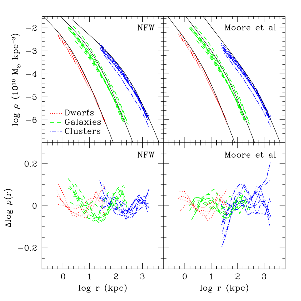
Figure 1: Spherically-averaged density profiles of all our simulated halos. Densities are computed in radial bins of equal logarithmic width and are shown from the innermost converged radius ($r_{\rm conv}$) out to about the virial radius of each halo ($r_{200}$). Our simulations target halos in three distinct mass groups: “dwarf”, “galaxy”, and “cluster” halos. These groups span more than five decades in mass. Thick solid lines in the top panels illustrate the expected halo profile for each mass range according to the fitting formula proposed by NFW (top-left) or M99 (top-right). Bottom panels indicate the deviation from the best fit achieved for each individual halo (simulation minus fit) with the NFW profile (eq. 1) or with its modified form, as proposed by M99 (eq. 2).

The top panels of Figure 1 show the density profiles, $\rho(r)$, of the nineteen simulated halos in our sample. In physical units, the profiles split naturally into three groups: from left to right, “dwarf” (dotted), “galaxy” (dashed), and “cluster” (dot-dashed) halos, respectively. Each profile is shown from the virial radius, $r_{200}$, down to the innermost converged radius, $r_{\rm conv}$; a convention that we shall adopt in all figures throughout this paper.

The thick solid lines in the top-left panel show the NFW profiles (eq. 1) expected for halos in each group, with parameters chosen according to the prescription of Eke, Navarro & Steinmetz (2001). Note that these NFW curves are not best fits to any of the simulations, but that they still capture reasonably well the shape and normalization of the density profiles of the simulated halos.

The top right panel of Figure 1 is similar to the top left one, but the comparison is made here with the modified form of the NFW profile proposed by M99 (eq. 2). There is no published prescription specifying how to compute the numerical parameters of this formula for halos of given mass, so the three profiles shown in this panel are just “eyeball” fits to one halo in each group. Like the NFW profile, the M99 formula also appears to describe reasonably well the gently-curving density profiles of $\Lambda$CDM halos.

Figure 1 thus confirms a number of important trends that were already evident in prior simulation work.

• $\Lambda$CDM halo density profiles deviate significantly from simple power laws, and steepen systematically from the center outwards; they are shallower than isothermal near the center and steeper than isothermal near the virial radius.

• There is no indication of a well defined central “core” of constant density; the dark matter density keeps increasing all the way in, down to the innermost resolved radius.

• Simple formulae such as the NFW profile (eq. 1) or the M99 formula (eq. 2) appear to describe the mass profile of all halos reasonably well, irrespective of mass, signaling a “universal” profile shape. Properly scaled, a dwarf galaxy halo is almost indistinguishable from a galaxy cluster halo.

We elaborate further on each of these conclusions in what follows.

3.1.1 NFW vs M99 fits

Are the density profiles of $\Lambda$CDM halos described better by the NFW formula (eq. 1) or by the modification proposed by M99 (eq. 2)? The answer may be seen in the bottom panels of Figure 1. These panels show the deviations (simulation minus fit) from the best fits to the density profiles of each halo using the NFW profile or the M99 profile. These fits are obtained by straightforward $\chi^{2}$ minimization, assigning equal weight to each radial bin. This is done because the statistical (Poisson) uncertainty in the determination of the density within each bin is negligible (each bin contains from several thousand to several hundred thousand particles) so the remaining uncertainties are likely to be dominated by systematics, such as the presence of substructure, varying asphericity, as well as numerical error, whose radial dependence is difficult to assess quantitatively (see P03).

As shown in the bottom panels of Figure 1, there is significant variation in the shape of the density profile from one halo to another. Some systems are fit better by eq. 1 than by eq. 2, and the reverse is true in other cases. Over the radial range resolved by the simulations, $\rho(r)$ deviates from the best fits by less than $\sim 50\%$. NFW fits tend to underestimate the density in the inner regions of most halos; by up to $35\%$ at the innermost resolved point. M99 fits, on the other hand, seem to do better for low mass halos, but tend to overestimate the density in the inner regions of cluster halos by up to $60\%$. We have explicitly checked that these conclusions are robust to reasonable variation in the binning used to construct the density profiles, as well as in the adopted minimization procedure.

This level of accuracy may suffice for a number of observational applications, with the proviso that comparisons are restricted to radii where numerical simulations are reliable; i.e., $r_{\rm conv}<r<r_{200}$. Deviations from the best fits increase systematically towards the center, so it is likely that extrapolations of either fitting formula to radii much smaller than $r_{\rm conv}$ will incur substantial error. We discuss below (§ 3.6) possible modifications to the fitting formulae that may minimize the error introduced by these extrapolations.

3.2 Circular Velocity Profiles

Many observations, such as disk galaxy rotation curves or strong gravitational lensing, are better probes of the cumulative mass distribution than of the differential density profile shown in Figure 1. Since cumulative profiles are subject to different uncertainties than differential ones, it is important to verify that our conclusions regarding the suitability of the NFW or M99 fitting formulae are also applicable to the cumulative mass distribution of $\Lambda$CDM halos.

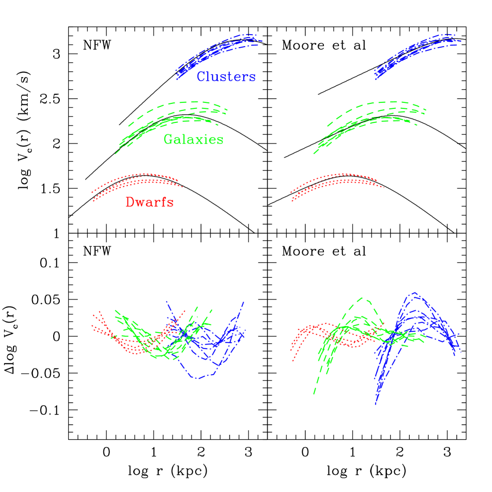
Figure 2: Spherically-averaged circular velocity ($V_{c}(r)=\sqrt{GM(r)/r}$) profiles of all our simulated halos. As in Figure 1, circular velocities are computed in radial bins of equal logarithmic width and are shown from the innermost converged radius ($r_{\rm conv}$) out to about the virial radius ($r_{200}$) of each halo. Our simulations target halos in three distinct mass groups: “dwarf”, “galaxy”, and “cluster” halos, spanning more than a factor of $\sim 50$ in velocity. Thick solid lines in the top panels illustrate the expected profile for each mass range according to the fitting formula proposed by NFW (top-left) or M99 (top-right). Bottom panels indicate the deviation from the best fit achieved for each individual halo (simulation minus fit) with the NFW profile (eq. 1) or with its modified form, as proposed by M99 (eq. 2).

The radial dependence of the spherically-averaged circular velocity profile of all halos in our series is shown in Figure 2. As in Figure 1, the thick solid curves in the top left (right) panel are meant to illustrate a typical NFW (M99) profile corresponding to dwarf, galaxy, and cluster halos, respectively. The bottom left and right panels show deviations from the best fit to each halo using the NFW or M99 profile, respectively. Both profiles reproduce the cumulative mass profile of the simulated halos reasonably well. The largest deviations seen are for the M99 fits, but they do not exceed $25\%$ over the radial range resolved in the simulations. NFW fits fare better, with deviations that do not exceed $10\%$.

As with the density profiles, the deviations between simulation and fits, although small, increase toward the center, suggesting that caution should be exercised when extrapolating these fitting formulae beyond the spatial region where they have been validated. This is important because observational data, such as disk galaxy rotation curves, often extend to regions inside the minimum convergence radius in these simulations.

3.3 Radial dependence of logarithmic slopes

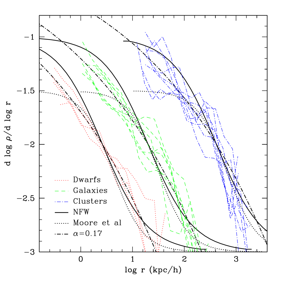
Figure 3: Logarithmic slope of the density profile of all halos in our sample, plotted versus radius. Thick solid and dotted curves illustrate the radial dependence of the slope expected from the NFW profile (eq. 1) and the modification proposed by M99 (eq. 2), respectively. Note that although both fitting formulae have well-defined asymptotic inner slopes ($-1$ and $-1.5$, respectively) there is no sign of convergence to a well-defined value of the central slope in the simulated halos. At the innermost converged radius, the simulated halo profiles are shallower than $-1.5$, in disagreement with the Moore et al profile. Also, inside the radius at which the slope equals $-2$, $r_{-2}$, the profiles appear to get shallower more gradually than in the NFW formula. A power-law radial dependence of the slope seems to fit the results of our simulations better; the dot-dashed lines indicate the predictions of the $\rho_{\alpha}$ profile introduced in eqs. 4 and  5 for $\alpha=0.17$. Best fits to individual halos yield $\alpha$ in the range $0.1$-$0.2$ (see Table LABEL:tab:fitpar).

We have noted in the previous subsections that systematic deviations are noticeable in both NFW and M99 fits to the mass profiles of simulated $\Lambda$CDM halos. NFW fits tend to underestimate the dark matter density near the center, whilst M99 fits tend to overestimate the circular velocity in the inner regions. The reason for this is that neither fitting formula fully captures the radial dependence of the density profile. We explore this in Figure 3, which shows the logarithmic slope, $d\ln\rho/d\ln r\equiv-\beta(r)$, of all simulated halos, as a function of radius. Although there is substantial scatter from halo to halo, a number of trends are robustly defined.

The first trend to note is that halo density profiles become shallower inward down to the innermost resolved radius, $r_{\rm conv}$ (the smallest radius plotted in Figure 3). We see no indication for convergence to a well defined asymptotic value of the inner slope in our simulated halos, neither to the $\beta_{0}=\beta(r=0)=1$ expected for the NFW profile (solid curves in Figure 3) nor to the $\beta_{0}=1.5$ expected in the case of M99 (dotted curves in same figure).

The second trend is that the radial dependence of the logarithmic slope deviates from what is expected from either the NFW or the M99 fitting formulae. Near $r_{\rm conv}$, the slopes are significantly shallower than $\beta_{0}=1.5$ (and thus in disagreement with the M99 formula) but they are also significantly steeper than expected from NFW fits. In quantitative terms, let us consider the slope well inside the characteristic radius, $r_{-2}$ (where the slope takes the “isothermal” value of $\beta(r_{-2})=2$). For cluster halos, for example, at $r=0.1\,r_{-2}$ ($\sim 50\,h^{-1}$ kpc) the average slope is approximately $-1.3$, whereas the NFW formula predicts $\sim-1.18$ and M99 predicts $\sim-1.5$. This is in agreement with the latest results of Fukushige, Kawai & Makino (2003), who also report profiles shallower than $r^{-1.5}$ at the innermost converged radius of their simulations. A best-fit slope of $r^{-1.3}$ was also reported by Moore et al (2001) for a dwarf galaxy halo (of mass similar to the Draco dwarf spheroidal), although that simulation was stopped at $z=4$, and might therefore not be directly comparable to the results we present here.

This discrepancy in the radial dependence of the logarithmic slope between simulations and fitting formulae is at the root of the different interpretations of the structure of the central density cusp proposed in the literature. For example, because profiles become shallower inward more gradually than in the NFW formula, modifications with more steeply divergent cusps (such as eq. 2) tend to fit density profiles (but not circular velocity profiles) better in the region interior to $r_{-2}$. This is not, however, a sure indication of a steeper cusp. Indeed, any modification to the NFW profile that results in a more gradual change in the slope inside $r_{-2}$ will lead to improved fits, regardless of the value of the asymptotic central slope. We show this explicitly below in § 3.6.

3.4 Maximum asymptotic slope

Conclusive proof that the central density cannot diverge as steeply as $\beta_{0}=1.5$ is provided by the total mass inside the innermost resolved radius, $r_{\rm conv}$. This is because, at any radius $r$, the mean density, $\bar{\rho}(r)$, together with the local density, $\rho(r)$, provide a robust upper limit to the asymptotic inner slope. This is given by $\beta_{\rm max}(r)=3(1-\rho(r)/{\bar{\rho}(r)})>\beta_{0}$, under the plausible assumption that $\beta$ is monotonic with radius.

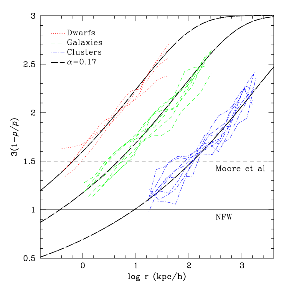
Figure 4: Maximum asymptotic inner slope compatible with the mean density interior to radius $r$, $\bar{\rho}(r)$, and with the local density at that radius, $\rho(r)$. This provides a robust limit to the central slope, $\beta_{0}<\beta_{\rm max}(r)=-3(1-\rho(r)/{\bar{\rho}(r)})$, under the plausible assumption that $\beta$ is monotonic with radius. Note that there is not enough mass within the innermost converged radius in our simulations to support density cusps as steep as $r^{-1.5}$. The asymptotic slope of the NFW profile, $\beta_{0}=1$, is still compatible with the simulated halos, although there is no convincing evidence for convergence to a well defined power-law behavior in any of our simulated halos. The thick dot-dashed curves illustrate the expected radial dependence of $\beta_{\rm max}$ for the $\rho_{\alpha}$ profile introduced in § 3.6, for $\alpha=0.17$.

Figure 4 shows $\beta_{\rm max}$ as a function of radius; clearly, except for possibly one dwarf system, no simulated halo has enough dark mass within $r_{\rm conv}$ to support cusps as steep as $r^{-1.5}$. The NFW asymptotic slope, corresponding to $\beta_{0}=1$, is still consistent with the simulation data, but the actual central value of the slope may very well be shallower. We emphasize again that there is no indication for convergence to a well defined value of $\beta_{0}$: density profiles become shallower inward down to the smallest resolved radius in the simulations.

3.5 A “universal” density profile

Figure 3 shows also that there is a well-defined trend with mass in the slope of the density profile measured at $r_{\rm conv}\sim 0.005$ to $0.01r_{200}$ (the innermost point plotted for each profile): $\beta(r_{\rm conv})\sim 1.1$ for clusters, $\sim 1.2$ for galaxies, and $\sim 1.35$ for dwarfs. A similar trend was noted by Jing & Suto (2000), who used it to argue against a “universal” density profile shape. However, as discussed by Klypin et al (2001), this is just a reflection of the trend between the concentration of a halo and its mass. It does not indicate any departure from similarity in the profile shape. Indeed, one does not expect the profiles of halos of widely different mass, such as those in our series, to have similar slopes at a constant fraction of the virial radius. Rather, if the density profiles are truly self-similar, slopes ought to coincide at fixed fractions of a mass-independent radial scale, such as $r_{-2}$.

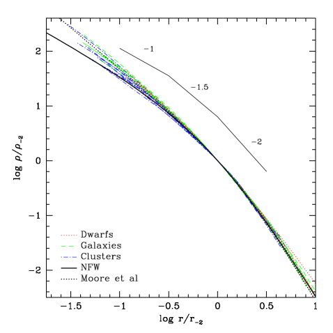
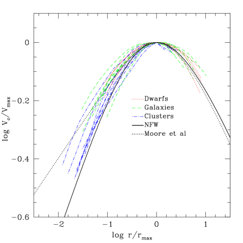
Figure 5: (a-left) Density profiles of all halos in our series, scaled to the radius, $r_{-2}$, where the local logarithmic slope of the density profile takes the isothermal value of $\beta=-d\log\rho/d\log r=2$. Densities are scaled to $\rho_{-2}=\rho(r_{-2})$. This figure shows that, with proper scaling, there is little difference in the shape of the density profile of halos of different mass, confirming the “universal” nature of the mass profile of $\Lambda$CDM halos. The NFW profile (eq. 1) is a fixed curve in these scaled units, and is shown with a thick solid line. The M99 formula (eq. 2) is shown with a dashed line. (b-right) Circular velocity profiles all halos in our series, scaled to the maximum velocity, $V_{\rm max}$, and to the radius at which it is reached, $r_{\rm max}$. Note the significant scatter from halo to halo, and also that the NFW and M99 profiles appear to bracket the extremes of the mass profile shapes of halos in our simulation series.

Figure 5a shows the striking similarity between the structure of halos of different mass when all density profiles are scaled to $r_{-2}$ and $\rho_{-2}\equiv\rho(r_{-2})$. The density profile of a dwarf galaxy halo then differs very little from that of a galaxy cluster $10^{5}$ times more massive. This demonstrates that spherically-averaged density profiles are approximately “universal” in shape; rarely do individual density profiles deviate from the scaled average by more than $\sim 50\%$.

In the scaled units of Figure 5, the NFW and M99 profiles are fixed, and are shown as solid and dotted curves, respectively. With this scaling, differences between density profiles are more evident than when best fits are compared, since the latter — by definition — minimize the deviations. In Figure 5a, for example, it is easier to recognize the “excess” of dark mass inside $r_{-2}$ relative to the NFW profile that authors such as M99 and Fukushige & Makino (1997, 2001, 2003) have (erroneously) interpreted as implying a steeply divergent density cusp.

The similarity in mass profile shapes is also clear in Figure 5b, which shows the circular velocity curves of all halos in our series, scaled to the maximum, $V_{\rm max}$ and to the radius where it is reached, $r_{\rm max}$. NFW and M99 are again fixed curves in these scaled units. This comparison is more relevant to observational interpretation, since rotation curve, stellar dynamical, and lensing tracers are all more directly related to $V_{c}(r)$ than to $\rho(r)$. Because of the reduced dynamic range of the y-axis, the scatter in mass profiles from halo to halo is more clearly apparent in the $V_{c}$ profiles; the NFW and M99 profiles appear to approximately bracket the extremes in the mass profile shapes of simulated halos. We discuss below a simple fitting formula that, with the aid of an extra parameter, is able to account for the variety of mass profile shapes better that either the NFW or M99 formula.

3.6 An improved fitting formula

Although the discussion in the previous subsections has concentrated on global deviations from simple fitting formulae such as NFW or M99, it is important to emphasize again that such deviations, although significant, are actually rather small. As shown in Figure 2, best NFW fits reproduce the circular velocity profiles to an accuracy of better than $\sim 10\%$ down to roughly $0.5\%$ of $r_{200}$. Although this level of accuracy may suffice for some observational applications, the fact that deviations increase inward and are maximal at the innermost converged point suggests the desirability of a new fitting formula better suited for extrapolation to regions beyond those probed reliably by simulations.

An improved fitting formula ought to reproduce: (i) the more gradual shallowing of the density profile towards the center; (ii) the apparent lack of evidence for convergence to a well-defined central power-law; and (iii) the significant scatter in profile shape from halo to halo. After some experimentation, we have found that a density profile where $\beta(r)$ is a power-law of radius is a reasonable compromise that satisfies these constraints whilst retaining simplicity;

$$\beta_{\alpha}(r)=-{d\ln\rho/d\ln r}=2\left({r/r_{-2}}\right)^{\alpha},$$ (4)

which corresponds to a density profile of the form,

$$\ln(\rho_{\alpha}/\rho_{-2})={(-2/\alpha)}[\left({r/r_{-2}}\right)^{\alpha}-1].$$ (5)

This profile has finite total mass (the density cuts off exponentially at large radius) and has a logarithmic slope that decreases inward more gradually than the NFW or M99 profile. The thick dot-dashed curves in Figures 3 and  4 show that eq. 5 (with $\alpha\sim 0.17$) does indeed reproduce fairly well the radial dependence of $\beta(r)$ and $\beta_{\rm max}(r)$ in simulated halos.

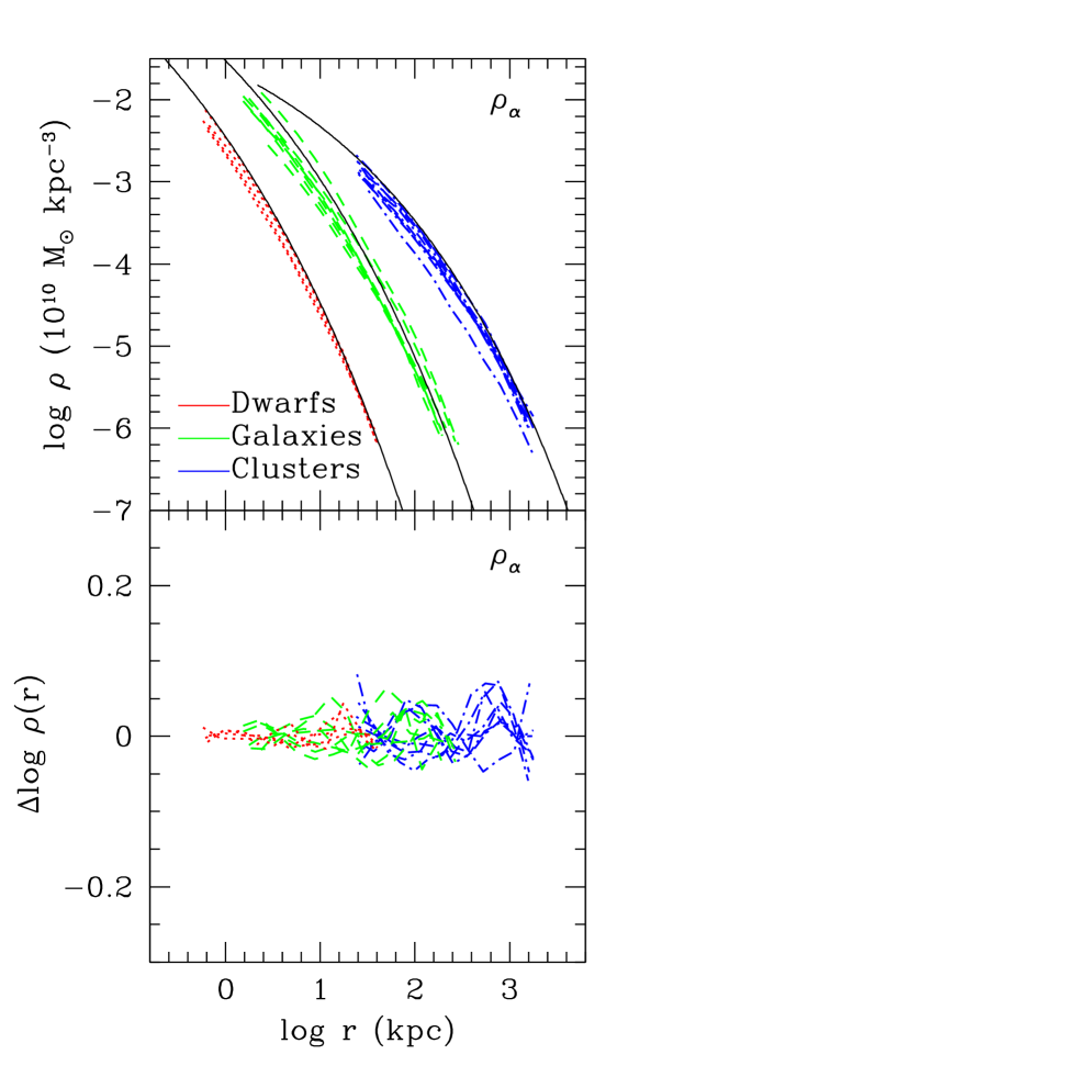
Figure 6: As Figure 1, but for the $\rho_{\alpha}$ fitting formula presented in eq. 5. Thick solid lines in the top panels illustrate the expected halo profile for each mass range according to the prescription proposed by NFW. Bottom panels indicate the deviation from the best $\rho_{\alpha}$ fit achieved for each individual halo, taking $\alpha$ as a free parameter. Note the improvement in the fits compared with those achieved with the NFW or M99 profile and shown in Figure 1.

Furthermore, adjusting the parameter $\alpha$ allows the profile to be tailored to each individual halo, resulting in improved fits. Indeed, as shown in Figure 6, eq. 5 reproduces the density profile of individual halos to better than $\sim 10\%$ over the reliably resolved radial range, and that there is no discernible radial trend in the residuals. This is a significant improvement over NFW or M99 fits, where the maximum deviations were found at the innermost resolved radius. The best-fit values of $\alpha$ (in the range $0.1$ - $0.2$) show no obvious dependence on halo mass, and are listed in Table LABEL:tab:fitpar. The average $\alpha$ is $0.172$ and the dispersion about the mean is $0.032$.

We note that the $\rho_{\alpha}$ profile is not formally divergent, and converges to a finite density at the center, $\rho_{0}=e^{2/\alpha}\,\rho_{-2}\sim 6\times 10^{5}\rho_{-2}$ (for $\alpha=0.15$). It is unclear at this point whether such asymptotic behavior is a true property of $\Lambda$CDM halos or simply an artifact of the fitting formula that results from choosing $\beta_{0}=0$ in eq. 4. The simulations show no evidence for convergence to a well-defined central value for the density, but even in the best-resolved cases they only probe regions where densities do not exceed $\sim 10^{2}\,\rho_{-2}$. This is, for $\alpha$ in the range $0.1$ - $0.2$, several orders of magnitude below the maximum theoretical limit in eq. 5.

We note as well that the convergence to $\beta_{0}=0$ is quite slow for the values of $\alpha$ favored by our fits. Indeed, for $\alpha=0.1$, the logarithmic slope only reaches a value significantly shallower than the NFW asymptotic slope at radii that are well inside the convergence radius of our simulations; for example, $\beta_{\alpha}(r)$ only reaches $0.5$ at $r=9.5\times 10^{-7}\,r_{-2}$, corresponding to $r\sim 0.01$ pc for galaxy-sized halos. This implies that the $\rho_{\alpha}$ profile is in practice “cuspy” for most astrophysical applications. Establishing conclusively whether $\Lambda$CDM halos actually have divergent inner density cusps is a task that awaits simulations with much improved resolution than those presented here.

3.7 Comparison between fitting formulae

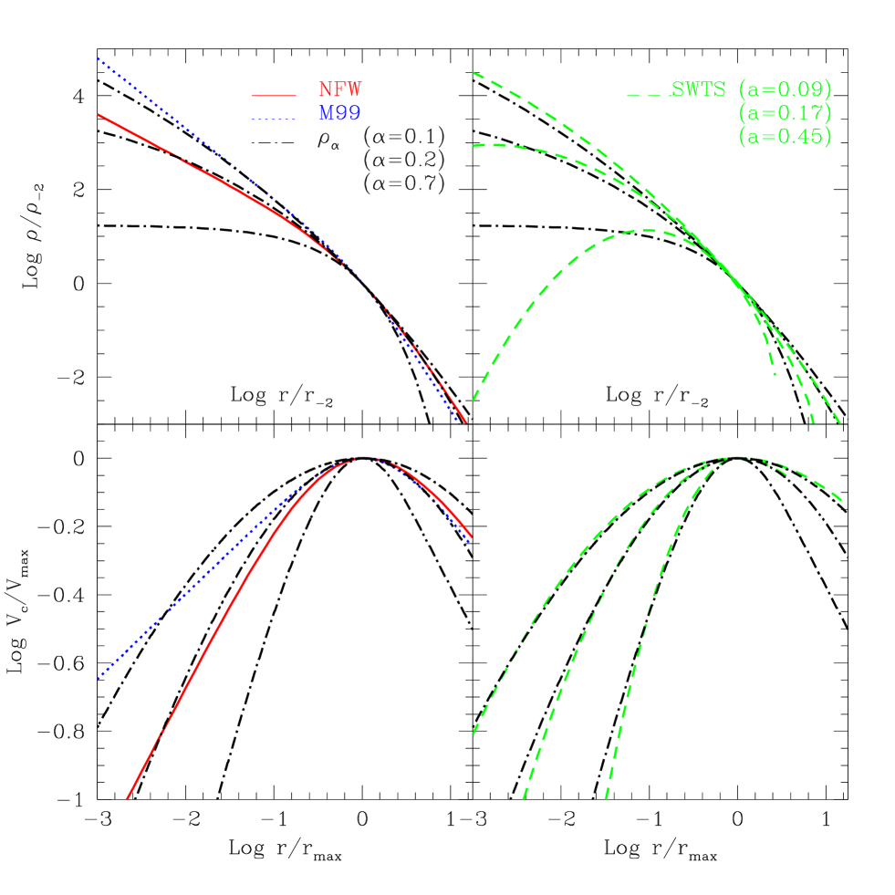
Figure 7: Comparison between the density (top) and circular velocity (bottom) profiles corresponding to four different fitting formulae: NFW (solid curves, eq. 1), M99 (dotted curves, eq. 2), SWTS (dashed curves, eq. 6), and $\rho_{\alpha}$ (dot-dashed curves, eq. 5). Circular velocity profiles are scaled to the maximum, $V_{\rm max}$, and to the radius where that is reached, $r_{\rm max}$. Density profiles are scaled as in Figure 5. Note that, despite having a finite central density, the $\rho_{\alpha}$ formula matches, for about 3 decades in radius, the NFW profile (for $\alpha=0.2$) or the M99 profile (for $\alpha=0.1$, see top left panel). It also matches closely the SWTS “parabolic” circular velocity profiles intended to reproduce substructure halos (see bottom right panel); the $V_{c}$ profile with $\alpha=0.7$ is very similar to the SWTS profile with $a=0.45$, the median value of the fits to substructure halos reported by SWTS. See text for further discussion.

Figure 7 compares the density and circular velocity profiles implied by the $\rho_{\alpha}$ formula (eq. 5) with the NFW and M99 profiles (left panels), as well as with the fitting formula proposed by Stoehr et al (2002, hereafter SWTS) to describe the structure of substructure halos (right panels).

The top left panel of Figure 7 shows that, despite its finite central density, the $\rho_{\alpha}$ profile can approximate fairly well both an NFW profile (for $\alpha\sim 0.2$) and an M99 profile (for $\alpha\sim 0.1$) for over three decades in radius. The circular velocity profile for $\alpha=0.2$ is likewise quite similar to NFW’s (bottom left panel of Figure 7), but the similarity to the shape of the M99 $V_{c}$ profile is less for all values of $\alpha$.

Interestingly, the $V_{c}$ profiles corresponding to $\rho_{\alpha}$ resemble parabolae in a $\log$-$\log$ plot, and thus may be used to approximate as well the mass profiles of substructure halos, as discussed by SWTS. This is demonstrated in the bottom right panel of Figure 7, where we show that the $V_{c}$ profiles corresponding to $\alpha=0.1$, $0.2$, and $0.7$, are very well approximated by the SWTS formula,

$$\log(V_{c}/V_{\rm max})=-a[\log(r/r_{\rm max})]^{2},$$ (6)

for $a=0.09$, $0.17$, and $0.45$, respectively. The latter value ($a=0.45$, or $\alpha=0.7$) corresponds to the median of the best SWTS fits to the mass profile of substructure halos. Note that this is quite different from the $\alpha\sim 0.1$ - $0.2$ required to fit isolated $\Lambda$CDM halos (see Table LABEL:tab:fitpar).

It might actually be preferable to adopt the $\rho_{\alpha}$ profile rather than the SWTS formula for describing substructure halos, since $\rho_{\alpha}(r)$ is monotonic with radius and extends over all space. This is not the case for SWTS, as shown in the top-right panel of Figure 7. The SWTS density profiles are “hollow” (i.e., the density has a minimum at the center), and extend out to a maximum radius, given by $e^{1/4a}\,r_{\rm max}$. This is because the circular velocity in the outer regions of the SWTS formula fall off faster than Keplerian, and therefore the corresponding density becomes formally negative at a finite radius.

The $\rho_{\alpha}$ profile thus appears versatile enough to reproduce, with a single fitting parameter, the structure of $\Lambda$CDM halos and of their substructure. Since $\rho_{\alpha}$ captures the inner slopes better than either the NFW or M99 profile, it is also likely to be a safer choice should extrapolation of the mass profile beyond the converged radius prove necessary. We end by emphasizing, however, that all simple fitting formulae have shortcomings, and that direct comparison with simulations rather than with fitting formulae should be attempted whenever possible.

3.8 Scaling parameters

The application of fitting formulae such as the one described above requires a procedure for calculating the characteristic scaling parameters for a given halo mass, once the power spectrum and cosmological parameters are specified. NFW developed a simple procedure for calculating the parameters corresponding to halos of a given mass. Because of the close relationship between the scale radius, $r_{s}$, and characteristic density, $\rho_{s}$, of the NFW profile and the $r_{-2}$ and $\rho_{-2}$ parameters of eq. 5, we can use the formalism developed by NFW to compute the expected values of these parameters in a given cosmological model.

NFW interpreted the characteristic density of a halo as reflecting the density of the universe at a suitably defined time of collapse. Their formalism assigns to each halo of mass $M$ (identified at $z=0$) a collapse redshift, $z_{\rm coll}(M,f)$ defined as the epoch when half the mass of the halo was first contained in progenitors more massive than a certain fraction $f$ of the final mass. With this definition, and once $f$ has been chosen, $z_{\rm coll}$ can be computed using the Press-Schechter theory (e.g., Lacey & Cole 1993). The NFW model then assumes that the characteristic density of a halo (i.e., $\rho_{s}$ in eq. 1) is proportional to the mean density of the universe at $z_{\rm coll}$.

The redshift dependence of the characteristic density was first probed in detail by Bullock et al (2001, hereafter B01), who proposed a modification to NFW’s model in which, for a given halo mass, the scale radius, $r_{s}$, remains approximately constant with redshift. Eke, Navarro & Steinmetz (2001, hereafter ENS), on the other hand, argued that the characteristic density of a halo is determined by the amplitude and shape of the power spectrum, as well as by the universal expansion history. Their formalism reproduces nicely the original results of NFW as well as the redshift dependence pointed out by B01, and is applicable to more general forms of the power spectrum, including the “truncated” power spectra expected in scenarios such as warm dark matter (see ENS for more details).

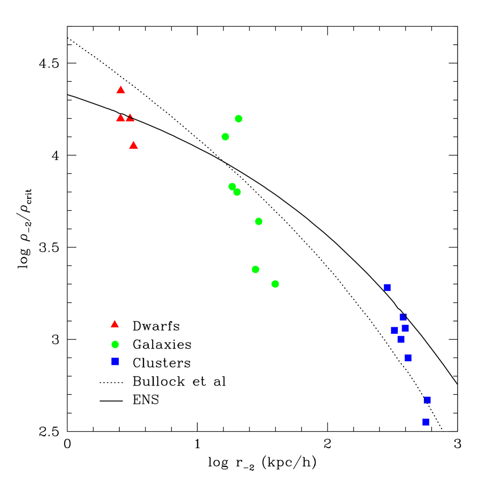
Figure 8: The radius, $r_{-2}$, where the logarithmic slope of the density profile takes the “isothermal” value, $\beta(r_{-2})=2$, plotted versus the local density at that radius, $\rho_{-2}=\rho(r_{-2})$, for all simulated halos in our series. This figure illustrates the mass dependence of the central concentration of dark matter halos: low mass halos are systematically denser than their more massive counterparts. Solid and dotted lines indicate the scale radius-characteristic density correlation predicted by the formalisms presented by Eke, Navarro & Steinmetz (2001) and Bullock et al (2001). These parameters may be used, in conjunction with eq. 5, to predict the mass profile of $\Lambda$CDM halos.

We have used the ENS and B01 formalisms to predict the halo mass dependence of the scaling parameters, $\rho_{-2}$ and $r_{-2}$, and we compare the results with our simulations in Figure 8. The ENS prediction is shown by the solid line whereas the dotted line shows that of B01. Both formalisms reproduce reasonably well the trend seen in the simulations, so that one can use either, in conjunction with eq. 5 (with $\alpha$ in the range 0.1-0.2), to predict the structure of a $\Lambda$CDM halo. A simple code that computes $r_{-2}$ and $\rho_{-2}$ as a function of mass in various cosmological models is available upon request from the authors. Existing codes that compute NFW halo parameters as a function of mass and of other cosmological parameters may also be used, noting that $\rho_{-2}=\rho_{s}/4$ and that $r_{-2}=r_{s}$.

Finally, we note that neither formalism captures perfectly the mass dependence of the characteristic density; small but significant deviations, as well as a sizable scatter, are evident in Figure 8. Dwarf galaxy halos appear to be less concentrated than predicted by the formalism proposed by B01; a similar observation applies to cluster halos when compared to ENS’ predictions. Such shortcomings should be considered when deriving cosmological constraints from fits to observational data (see, e.g., Zentner & Bullock 2002, McGaugh et al 2003); and suggest again that direct comparison between observation and simulations is preferable to the use of fitting formulae.

4 Summary

We have analyzed the mass profile of $\Lambda$CDM halos in a series of simulations of high mass, spatial, and temporal resolution. Our series targets halos spanning five decades in mass: “dwarf” galaxy halos with virial circular velocities of order $V_{200}\sim 30$ km s^-1; “galaxy”-sized halos with $V_{200}\sim 200$ km s^-1; and “cluster” halos with $V_{200}\sim 1200$ km s^-1. Each of the nineteen halos in our series was simulated with comparable numerical resolution: they have between $8\times 10^{5}$ and $4\times 10^{6}$ million particles within the virial radius, and have been simulated following the “optimal” prescription for time-stepping and gravitational softening laid down in the numerical convergence study of P03.

The high resolution of our simulations allows us to probe the inner properties of the mass profiles of $\Lambda$CDM halos, down to $\sim 0.5\%$ of $r_{200}$ in our best resolved runs. These results have important implications for the structure of the inner cusp in the density profile and resolve some of the disagreements arising from earlier simulation work. Our main conclusions may be summarized as follows.

• $\Lambda$CDM halo density profiles are “universal” in shape: i.e., a simple fitting formula reproduces the structure of all simulated halos, regardless of mass. Both the NFW profile and the profile proposed by M99 describe the density and circular velocity profiles of simulated halos reasonably well. Best NFW fits to the circular velocity profiles deviate by less than $10\%$ over the region which is well resolved numerically. Best M99 fits reproduce circular velocity profiles to better than $25\%$ over the same region. It should be noted, however, that the deviations increase inwards and are typically maximal at the innermost resolved radius, a result that warns against extrapolating to smaller radii with these fitting formulae.

• $\Lambda$CDM halos appear to be “cuspy”: i.e., the dark matter density increases monotonically towards the center with no evidence for a well-defined “core” of constant density. We find no evidence, however, for a central asymptotic power-law bin the density profiles. These become progressively shallow inwards and are significantly shallower than isothermal at the innermost resolved radius, $r_{\rm conv}$. At $r\sim 0.01\,r_{200}$, the average slope of “cluster”, “galaxy” and “dwarf” halos halos is $\beta(r_{\rm conv})\sim 1.1$, $\sim 1.2$, and $\sim 1.35$, respectively. This is steeper than predicted by the NFW profile but shallower than the asymptotic slope of the M99 profile.

• The density and enclosed mass at $r_{\rm conv}$ may be used to derive an upper limit on any asymptotic value of the inner slope. Cusps as steep as $\beta_{0}=1.5$ are confidently ruled out in essentially all cases; the asymptotic slope of the NFW profile ($\beta_{0}=1$) is still consistent with our data. The radial dependence of $\beta(r)$ differs from that of the NFW profile, however, decreasing more slowly with decreasing radius than is predicted. For some scalings of the NFW fitting formula to the numerical data, this shape difference appears as a dark matter “excess” near the center which has (erroneously) been interpreted indicating a steeply divergent density cusp.

• A simple formula where $\beta(r)$ is a power law of radius reproduces the gradual radial variation of the logarithmic slope and its apparent failure to converge to any specific asymptotic value (eq. 5). This formula leads to much improved fits to the density profiles of simulated halos, and may prove a safer choice when comparison with observation demands extrapolation below the innermost converged radii of the simulations.

Our study demonstrates that, although simple fitting formulae such as NFW are quite accurate in describing the global structure of $\Lambda$CDM halos, one should be aware of the limitations of these formulae when interpreting observational constraints. Extrapolation beyond the radial range where these formulae have been validated is likely to produce substantial errors. Proper account of the substantial scatter in halo properties at a given halo mass also appears necessary when assessing the consistency of observations with a particular cosmological model. Direct comparison between observations and simulations (rather than with fitting formulae) is clearly preferable whenever possible. Given the computational challenge involved in providing consistent, robust, and reproducible theoretical predictions for the inner structure of CDM halos it is likely that observational constraints will exercise to the limit our hardware and software capabilities for some time to come.

This work has been supported by computing time generously provided by the High Performance Computing Facility at the University of Victoria, as well as by the Edinburgh Parallel Computing Centre and by the Institute for Computational Cosmology at the University of Durham. Expert assistance by Colin Leavett-Brown in Victoria and Lydia Heck in Durham is gratefully acknowledged. JFN is supported by the Alexander von Humboldt Foundation, the Natural Sciences and Engineering Research Council of Canada, and the Canadian Foundation for Innovation.

Table 1: Parameters of the parent cosmological simulations

Label	$L_{\rm box}$	$z_{i}$	$m_{p}$	$\epsilon$	CODE
	[$h^{-1}$ Mpc]		[$h^{-1}\,M_{\odot}$]	[$h^{-1}$ kpc]
ENS01	$32.5$	$49.0$	$1.36\times 10^{9}$	$10$	AP3M
SGIF-128	$35.325$	$49.0$	$1.75\times 10^{9}$	$10$	GADGET
$\Lambda$CDM-512	$479.0$	$36.0$	$6.82\times 10^{10}$	$30$	GADGET

Table 2: Main parameters of resimulated halos

Label	$z_{i}$	$\epsilon$	$N_{200}$	$M_{200}$	$r_{200}$	$V_{200}$	$r_{\rm conv}$	CODE
		[$h^{-1}$ kpc]		[$h^{-1}\,M_{\odot}$]	[$h^{-1}$ kpc]	[km s-1]	[$h^{-1}$ kpc]
D1	$74$	$0.0625$	$784980$	$7.81\times 10^{9}$	$32.3$	$32.3$	$0.34$	GADGET
D2	$49$	$0.0625$	$778097$	$9.21\times 10^{9}$	$34.1$	$34.1$	$0.37$	GADGET
D3	$49$	$0.0625$	$946421$	$7.86\times 10^{9}$	$32.3$	$32.3$	$0.33$	GADGET
D4	$49$	$0.0625$	$1002098$	$9.72\times 10^{9}$	$34.7$	$34.7$	$0.32$	GADGET
G1	$49$	$0.15625$	$3447447$	$2.29\times 10^{12}$	$214.4$	$214.4$	$1.42$	GADGET
G2	$49$	$0.5$	$4523986$	$2.93\times 10^{12}$	$232.6$	$232.6$	$1.25$	PKDGRAV
G3	$49$	$0.45$	$2661091$	$2.24\times 10^{12}$	$212.7$	$212.7$	$1.65$	PKDGRAV
G4	$49$	$0.3$	$3456221$	$1.03\times 10^{12}$	$164.0$	$164.0$	$1.01$	PKDGRAV
G5	$49$	$0.35$	$3913956$	$1.05\times 10^{12}$	$165.0$	$165.0$	$1.02$	PKDGRAV
G6	$49$	$0.35$	$3739913$	$9.99\times 10^{11}$	$162.5$	$162.5$	$1.03$	PKDGRAV
G7	$49$	$0.35$	$3585676$	$9.58\times 10^{11}$	$160.3$	$160.3$	$1.02$	PKDGRAV
C1	$36$	$5.0$	$1565576$	$7.88\times 10^{14}$	$1502.1$	$1502.1$	$16.8$	GADGET
C2	$36$	$5.0$	$1461017$	$7.36\times 10^{14}$	$1468.1$	$1468.1$	$16.9$	GADGET
C3	$36$	$5.0$	$1011918$	$5.12\times 10^{14}$	$1300.6$	$1300.6$	$16.1$	GADGET
C4	$36$	$5.0$	$1050402$	$5.31\times 10^{14}$	$1316.7$	$1316.7$	$15.9$	GADGET
C5	$36$	$5.0$	$1199299$	$6.05\times 10^{14}$	$1375.5$	$1375.5$	$16.2$	GADGET
C6	$36$	$5.0$	$1626161$	$8.19\times 10^{14}$	$1521.1$	$1521.1$	$15.5$	GADGET
C7	$36$	$5.0$	$887837$	$4.50\times 10^{14}$	$1245.8$	$1245.8$	$16.4$	GADGET
C8	$36$	$5.0$	$1172850$	$5.92\times 10^{14}$	$1365.4$	$1365.4$	$16.8$	GADGET

Table 3: Fit and structural parameters of resimulated halos

Label	$r_{-2}$	$\rho_{-2}$	$r_{\rm max}$	$V_{\rm max}$	$r_{s}$	$\rho_{s}$	$r_{M}$	$\rho_{M}$	$\alpha$
	[$h^{-1}$ kpc]	[$\rho_{\rm crit}$]	[$h^{-1}$ kpc]	[km s-1]	[$h^{-1}$ kpc]	[$\rho_{\rm crit}$]	[$h^{-1}$ kpc]	[$\rho_{\rm crit}$]
D1	$3.23$	$1.12e4$	$6.07$	$39.1$	$2.59$	$7.03e4$	$5.38$	$7.58e3$	$0.164$
D2	$3.04$	$1.58e4$	$6.64$	$44.2$	$2.43$	$9.61e4$	$2.27$	$1.17e5$	$0.211$
D3	$2.57$	$1.58e4$	$6.35$	$36.9$	$2.94$	$5.01e4$	$4.05$	$2.51e4$	$0.122$
D4	$2.57$	$2.24e4$	$4.27$	$45.7$	$2.06$	$1.49e5$	$2.18$	$1.36e5$	$0.166$
G1	$18.5$	$6.76e3$	$23.7$	$1.95e2$	$23.2$	$4.06e4$	$19.4$	$8.43e4$	$0.142$
G2	$28.0$	$2.40e3$	$68.5$	$1.78e2$	$16.8$	$1.13e5$	$19.4$	$8.43e4$	$0.191$
G3	$20.2$	$6.31e3$	$43.4$	$1.96e2$	$28.0$	$1.52e4$	$47.3$	$8.24e3$	$0.142$
G4	$29.6$	$4.37e3$	$63.4$	$2.49e2$	$12.3$	$6.78e4$	$16.8$	$3.44e4$	$0.177$
G5	$20.7$	$1.58e4$	$67.7$	$2.91e2$	$13.8$	$5.20e4$	$15.3$	$4.23e4$	$0.184$
G6	$39.6$	$2.00e3$	$96.4$	$2.26e2$	$15.3$	$3.79e4$	$20.7$	$2.03e4$	$0.171$
G7	$16.4$	$1.26e4$	$29.9$	$1.94e2$	$13.4$	$6.22e4$	$14.9$	$5.15e4$	$0.138$
C1	$5.84e2$	$4.68e2$	$1.03e3$	$1.48e3$	$440$	$3.36e3$	$661$	$1.58e3$	$0.133$
C2	$3.95e2$	$1.15e3$	$9.99e2$	$1.51e3$	$362$	$5.17e3$	$396$	$4.46e3$	$0.215$
C3	$3.27e2$	$1.12e3$	$6.15e2$	$1.38e3$	$249$	$9.07e3$	$278$	$7.44e3$	$0.188$
C4	$4.16e2$	$7.94e2$	$6.57e2$	$1.38e3$	$315$	$5.47e3$	$339$	$4.91e3$	$0.161$
C5	$2.87e2$	$1.91e3$	$6.48e2$	$1.42e3$	$271$	$8.45e3$	$326$	$5.88e3$	$0.215$
C6	$3.82e2$	$1.32e3$	$6.94e2$	$1.64e3$	$297$	$8.70e3$	$302$	$8.75e3$	$0.203$
C7	$5.69e2$	$3.55e2$	$1.25e3$	$1.25e3$	$283$	$3.92e3$	$475$	$2.11e3$	$0.129$
C8	$3.68e2$	$1.00e3$	$9.35e2$	$1.44e3$	$361$	$4.41e3$	$345$	$5.04e3$	$0.219$

References

- Bardeen, Bond, Kaiser, & Szalay (1986) Bardeen, J. M., Bond, J. R., Kaiser, N., & Szalay, A. S. 1986, ApJ, 304, 15
- (2) Binney, J. 2003, MNRAS, submitted (astro-ph/0311155).
- Bullock et al. (2001) Bullock, J. S., Kolatt, T. S., Sigad, Y., Somerville, R. S., Kravtsov, A. V., Klypin, A. A., Primack, J. R., & Dekel, A. 2001, MNRAS, 321, 559
- Calcáneo-Roldán & Moore (2000) Calcáneo-Roldán, C. & Moore, B. 2000, Phys. Rev. D, 62, 123005
- Cole & Lacey (1996) Cole, S. & Lacey, C. 1996, MNRAS, 281, 716
- Crone, Evrard, & Richstone (1994) Crone, M. M., Evrard, A. E., & Richstone, D. O. 1994, ApJ, 434, 402
- Davis, Efstathiou, Frenk, & White (1985) Davis, M., Efstathiou, G., Frenk, C. S., & White, S. D. M. 1985, ApJ, 292, 371
- Debattista & Sellwood (1998) Debattista, V. P. & Sellwood, J. A. 1998, ApJ, 493, L5
- Dubinski & Carlberg (1991) Dubinski, J. & Carlberg, R. G. 1991, ApJ, 378, 496
- Eke, Navarro, & Steinmetz (2001) Eke, V. R., Navarro, J. F., & Steinmetz, M. 2001, ApJ, 554, 114
- Flores & Primack (1994) Flores, R. A. & Primack, J. R. 1994, ApJ, 427, L1
- Frenk, White, Davis, & Efstathiou (1988) Frenk, C. S., White, S. D. M., Davis, M., & Efstathiou, G. 1988, ApJ, 327, 507
- Fukushige & Makino (1997) Fukushige, T. & Makino, J. 1997, ApJ, 477, L9
- Fukushige & Makino (2001) Fukushige, T. & Makino, J. 2001, ApJ, 557, 533
- Fukushige & Makino (2003) Fukushige, T. & Makino, J. 2003, ApJ, 588, 674
- Fukushige, Kawai & Makino (2003) Fukushige, T. , Kawai, A. & Makino, J. 2003, astro-ph/0306203
- Ghigna et al. (2000) Ghigna, S., Moore, B., Governato, F., Lake, G., Quinn, T., & Stadel, J. 2000, ApJ, 544, 616
- Hayashi et al (2003) Hayashi, E., Navarro, J.F., Jenkins, A., Power, C., Frenk, C.S., White, S.D.M., Springel, V., Stadel, J., Quinn, T.R. 2003, MNRAS, submitted (astro-ph/0310576)
- Huss, Jain, & Steinmetz (1999) Huss, A., Jain, B., & Steinmetz, M. 1999, ApJ, 517, 64
- Jing & Suto (2000) Jing, Y. P. & Suto, Y. 2000, ApJ, 529, L69
- Klypin, Kravtsov, Bullock, & Primack (2001) Klypin, A., Kravtsov, A. V., Bullock, J. S., & Primack, J. R. 2001, ApJ, 554, 903
- Lacey & Cole (1993) Lacey, C. & Cole, S. 1993, MNRAS, 262, 627
- McGaugh & de Blok (1998) McGaugh, S. S. & de Blok, W. J. G. 1998, ApJ, 499, 41
- McGaugh, Barker, & de Blok (2003) McGaugh, S. S., Barker, M. K., & de Blok, W. J. G. 2003, ApJ, 584, 566
- Moore (1994) Moore, B. 1994, Nature, 370, 629
- Moore et al. (1999) Moore, B., Quinn, T., Governato, F., Stadel, J., & Lake, G. 1999, MNRAS, 310, 1147
- Moore et al. (2001) Moore, B., Calcáneo-Roldán, C., Stadel, J., Quinn, T., Lake, G., Ghigna, S., & Governato, F. 2001, Phys. Rev. D, 64, 63508
- Navarro, Frenk, & White (1996) Navarro, J. F., Frenk, C. S., & White, S. D. M. 1996, ApJ, 462, 563
- Navarro, Frenk, & White (1997) Navarro, J. F., Frenk, C. S., & White, S. D. M. 1997, ApJ, 490, 493
- Power et al. (2003) Power, C., Navarro, J. F., Jenkins, A., Frenk, C. S., White, S. D. M., Springel, V., Stadel, J., & Quinn, T. 2003, MNRAS, 338, 14
- Ricotti (2003) Ricotti, M. 2003, MNRAS, 344, 1237
- Seljak & Zaldarriaga (1996) Seljak, U. & Zaldarriaga, M. 1996, ApJ, 469, 437
- Springel, Yoshida, & White (2001) Springel, V., Yoshida, N., & White, S. D. M. 2001, New Astronomy, 6, 79
- Stadel (2001) Stadel, J. 2001, PhD thesis, University of Washington
- Stoehr, White, Tormen, & Springel (2002) Stoehr, F., White, S. D. M., Tormen, G., & Springel, V. 2002, MNRAS, 335, L84
- Subramanian, Cen, & Ostriker (2000) Subramanian, K., Cen, R., & Ostriker, J. P. 2000, ApJ, 538, 528
- Taylor & Navarro (2001) Taylor, J. E. & Navarro, J. F. 2001, ApJ, 563, 483
- Taylor & Silk (2003) Taylor, J. E. & Silk, J. 2003, MNRAS, 339, 505
- van den Bosch, Robertson, Dalcanton, & de Blok (2000) van den Bosch, F. C., Robertson, B. E., Dalcanton, J. J., & de Blok, W. J. G. 2000, AJ, 119, 1579
- Yoshida, Sheth, & Diaferio (2001) Yoshida, N., Sheth, R. K., & Diaferio, A. 2001, MNRAS, 328, 669
- Zentner & Bullock (2002) Zentner, A. R. & Bullock, J. S. 2002, Phys. Rev. D, 66, 43003