Time structure of muonic showers

Abstract

An analytical description of the time structure of the pulses induced by muons in air showers at ground level is deduced assuming the production distance distribution for the muons can be obtained elsewhere. The results of this description are compared against those obtained from simulated showers using AIRES. Major contributions to muon time delays are identified and a relation between the time structure and the depth distribution is unveiled.

I Introduction

One of the highest priorities in Astroparticle Physics has become the understanding of the origin, composition and energy spectrum of Ultra High Energy Cosmic Rays. Cosmic rays have been observed for a long time with energies known to exceed $10^{20}~{}$eV NW but the remarkably low flux at these energies makes their detection difficult. The air showers developing in the atmosphere from the interaction of these particles can be sampled at ground level with arrays of particle detectors. Alternatively the fluorescence light emitted by the nitrogen in the atmosphere can be collected by optical systems FE . Both types of experiments have confirmed the existence of cosmic rays of such high energies although there are discrepancies between the cosmic ray fluxes inferred by the different techniques AGASA ; HiRes .

The study of extensive air showers of the highest energies is difficult because the atmosphere is part of the detector and the interpretation of measurements is very indirect. The air shower is a complex chain of interactions resulting in a very large number of particles from which only sparse data samples are taken. From this sample, the properties of the primary particle must be deduced. We must rely on simplified models, or on complex numerical simulations, to infer these properties. These simulations have intrinsic and unavoidable uncertainties arising from interaction models that require untested extrapolations of low energy accelerator data. One of the complications arises because it is often very difficult to discern physical effects due to shower fluctuations or to primary composition from effects due to uncertainties in the interaction models. It is hoped that through redundancy in the observations, both the high energy models and the primary particle properties can be constrained.

Currently, the most important step in this direction is the development of the Auger Observatory. The southern part of the Observatory is now under construction in Argentina and will combine the fluorescence technique with a particle array of water Čerenkov tanks covering a surface area of 3000 km² Auger . The signal from the tanks is recorded with Flash Analog to Digital Converters and relative timing is synchronized using GPS technology to 10-20 ns. The time structure of the shower front is of crucial importance because the shower arrival direction in an array of particle detectors is determined from the relative arrival times of the signals. This is relatively easy since the shower front can be approximated by a plane but clearly there are curvature corrections to the front and the time structure of the signal and its fluctuations will have an impact on the precision of the reconstruction procedure. Understanding the time structure of the signal is most important for controlling the angular resolution. Last but not least, preliminary observations at the Auger Observatory are already revealing that the time structure of the tank signals carries much information ICRC and it is hoped that this new information can be used to answer fundamental questions such as primary composition.

As most high energy cosmic ray detectors are, or have been, arrays of particle detectors, the time structure of the shower front has been studied before Lapikens ; watson ; honda ; battistoni ; Kascade ; time1 . However most work is either experimental or phenomenological and there is not a great deal of knowledge about the time structure of signals in air showers from the theoretical side or of its relation to the shower parameters. In this work we study the time structure of the muon signal in air showers. Our work is based on ideas that have been introduced for the description of muon densities in inclined showers ModelPaper and is a natural extension of these ideas. Similar ideas have been developed in time1 ; time2 ; time3 .

Muons are naturally quite energetic when they reach the ground: otherwise they would have decayed in flight. As they have long radiation lengths they do not suffer many interactions in their travel path from the point where they are created to ground level. As a result if muons are present in the signal they define the earlier part of the shower front, i.e. its onset which is usually chosen to define the arrival time to be used in the reconstruction of the direction. Also muons have a much flatter lateral distribution than photons or electrons and they always dominate the signal at ground level for sufficiently large distances from the shower axis. Moreover, for inclined showers, they dominate the signal everywhere at ground level because the electromagnetic part of the shower, generated by the decay of neutral pions, is absorbed high in the atmosphere. Therefore, the description of the time structure of muons in air showers is of important practical interest for the reconstruction of air showers from measurements made in extensive air shower arrays. Understanding the muon part of the shower is not the complete story because there are important contributions to the shower signal due to electrons and photons. We will leave the study of the time structure of electrons and photons for future work. In this article we neglect the effect of the earth’s magnetic field, although it is known that magnetic effects are important for the description of muon densities at high zenith angles. We have checked that the time structure of muons is not affected by the magnetic field up to zenith angles of 80 degrees and more, depending on the strength of the magnetic field. Although our results are general, and we expect that they will be valid at all zenith angles, we will concentrate on the large zenith angles range, where the muon signal is more important.

The article is organized as follows. In Section II we present the main assumption on which this work is based and we develop an analytical description of muon energy distributions in air showers as a function of transverse distance. These will be used in the next section when the time structure of the shower front is addressed. In Section III we describe the two main sources of time delays associated with muons and we present a model for their description, discussing how it compares with the results obtained directly using simulations and the relevance of the magnetic field effects. In Section IV we apply the method to give general results about time distributions in air showers and in Section V we summarize and conclude.

II Towards an analytical description of muons in air showers

II.1 Factorization of Muon Distributions

Our starting point will be an approximate model for the description of the production of muons in air showers. As the shower develops, muons are in general produced at a range of altitudes with energies spanning a wide range and carrying some transverse momentum. We will assume that the muon distribution factorizes completely into a product of three independent distributions, the energy $f_{1}(E_{i})$, the transverse momentum $f_{2}(p_{t})$, and the distance to ground level $h(z)$

$$\frac{d^{3}N_{0}}{dp_{t}dE_{i}dz}=N_{0}f_{1}(E_{i})f_{2}(p_{t})h(z),$$ (1)

where $E_{i}$ and $p_{t}$ are the muon energy and transverse momentum at the production point, and $z$ is the distance from this point to ground level measured along the shower axis. The relation between $z$ and production altitude is straightforward but requires taking into account the curvature of the Earth for large zenith angle showers. The transverse momentum $p_{t}$ is defined with respect to the shower axis. Here the three distributions are normalized to 1 and $N_{0}$ corresponds to the total number of muons produced in the shower. After production we assume that the muons only undergo continuous energy loss and decay. This is known to be a reasonable approximation when the magnetic field is ignored. Hard catastrophic interactions, such as bremsstrahlung or pair production, are unlikely because the muon radiation length in air greatly exceeds the whole atmospheric depth even for the most inclined showers. The angular deviations of the muons reaching ground level due to multiple elastic scattering are negligible because the average muon energy at ground level is about 1 GeV for vertical showers and grows rapidly as the zenith angle increases to over 200 GeV for horizontal showers ModelPaper .

In Fig. 1 we show the geometry of the problem indicating the notation used. For a given distance to the shower axis, $r$, the actual distance traveled by the muon, is simply $l=\sqrt{r^{2}+(z-\Delta)^{2}}$, where $\Delta=r\tan\theta\cos\zeta$. $\theta$ is the shower zenith angle and $\zeta$ is the polar angle measured in a plane perpendicular to shower axis. We choose it to be zero for the case in which $l$ is a minimum. This system is natural for the description of the asymmetries of the problem and turns out to be most convenient.

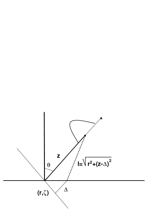
Figure 1: Schematic representation of the geometry and notation used for obtaining the arrival time distribution of muons in air showers. To describe the position at ground level of the muon signal we will use a cylindrical coordinate system $(z,r,\zeta)$ with the polar axis along the shower direction. Coordinates in the transverse plane $r$ and $\zeta$ are defined in such a way that $\zeta=0$ corresponds to the earliest part of the shower front. The dotted line represents the distance from first interaction (star) to the muon production point (dot). The dashed line corresponds to the path traveled by the muon, $l$, from which the time interval can be deduced. Since muons are observed as they reach ground level, observation at different angles $\zeta$ will correspond to different time delays because the path to ground is shortened by $\Delta$ (which is measured along shower axis).

The distribution of production distance for the muons, $h(z)$, depends on the details of the hadronic model, on the primary energy and on the primary chemical composition. We can parameterize it from Monte Carlo simulations. In this article we will use the results obtained with simulations run with the AIRES code Aires for an observation altitude of 1400 m, that of the southern Auger observatory, and using the QGSJET model for hadronic interactions QGSJET . For zenith angles above $60^{\circ}$ a Gaussian or a log-Gaussian distribution usually reproduces the production profile sufficiently well, but the distributions can be also described numerically if necessary. In Fig 2 we show the distribution of muon production distance as obtained from AIRES and our fit to a log-Gaussian distribution.

Figure 2: Production distance for proton showers of $10^{19}$ eV of $60^{\circ}$ and $80^{\circ}$ zenith angles as obtained using AIRES (histograms). Also shown is the result of a fit to a log-Gaussian distribution (continuous lines). The observation altitude was set to 1400 m.

In Table 1 we show the averages ($\log_{10}z_{0}$) and widths ($\sigma_{z}$) of log-Gaussian production distance fits performed for a number of showers at different zenith angles.

$\theta\;\;({\rm deg.})$	$z_{0}$(km)	$\log_{10}(z_{0}/{\rm km})$	$\sigma_{z}$
30	2.7	0.43	0.26
50	6.6	0.82	0.21
60	13.5	1.13	0.16
80	83.2	1.92	0.09

Table 1: Results of fits to log-Gaussian functions (in decimal base) to the production distance distributions obtained with Aires for proton showers and an observation altitude of 1400 m for different zenith angles. The last two entries are the logarithmic average $\log_{10}(z_{0}/{\rm km})=<\log_{10}(z/{\rm km})>$ and the width, $\sigma_{z}$. The second entry is $z_{0}$ the distance associated to the logarithmic average.

Equation 1 assumes that the transverse momentum distribution is independent of both the parent pion energy and its production altitude. Quite generally, this is equivalent to assuming that the transverse momentum distribution is a universal function which depends only on the hadronic interactions. When magnetic effects, muon interactions, and multiple elastic scattering are neglected, the transverse momentum distribution of the muons at production is the combination of that of the parent pion and that introduced through pion decay which is below 30 MeV/c and can be then ignored when compared to the typical momenta of hadronic interactions $\sim 200$ MeV/c. Fig. 3 illustrates the transverse momentum distribution of all the muons that reach ground level. The most distinctive feature that can be observed is a relatively sharp cutoff for large $p_{t}$. Particularly for low zenith angles this is close to an exponential cutoff. A good approximation for $f_{2}(p_{t})$ is given by

$$f_{2}(p_{t})\equiv\frac{1}{N_{0}}\frac{dN_{0}}{dp_{t}}=Bp_{t}^{\lambda}\exp(-p_{t}/Q),$$ (2)

where $\lambda\sim 1$, $Q\sim 170$ MeV/c is the characteristic momentum associated with hadronic interactions, and $B$ is a normalization constant.

Figure 3: Muon transverse momentum distribution at production for a proton shower of energy $10^{19}~{}$eV and $60^{\circ}$ zenith angle as obtained using AIRES. Only muons that reach an observation altitude of 1400 m are considered. The distribution of all muons (top curve) is compared to that obtained in different radial bins, [100,300] m, [30,100] m, [10,30] m (from second top to bottom).

The distribution obtained is actually similar to the transverse momentum distribution in hadronic interactions as could be expected if this was the only source of transverse momentum. The main corrections to this simplification arise through the cumulative effect of transverse momenta acquired in multiple scattering of parent hadrons before the final hadron (usually a pion) decays into a muon. This cascading effect contributes to enhance the high-$p_{t}$ tail of the momentum distribution, but fortunately it has little effect on the shape of the bulk of the distribution. Indeed a small dependence of the average transverse momentum with production altitude can be understood, most likely because of this cumulative effect. As the width of the $p_{t}$ distribution greatly exceeds the magnitude of the shift in transverse momentum due to its correlation with production distance, one can effectively ignore this dependence which plays a secondary role.

Finally the energy distribution of the muons is known to be most affected by muon decay which, depending on the path length traveled by the muons from the production point to ground level, affects muons of different energies ModelPaper ; Lorenzo_icrc . One can, as a first approximation, use a fixed energy distribution at production, $f_{1}(E_{i})$, which then evolves because of continuous energy loss and decay in flight, to give the distribution at ground level, which is experimentally accessible with an air shower array. The most important effect is that there is a strong suppression of the distribution for muon ground energies below a low energy cutoff which is controlled by the travel distance for the muons. Clearly this cutoff is heavily dependent on zenith angle because the average distance to production increases rapidly from 1 km to 200 km as the zenith angle changes from vertical to horizontal.

Eq. 1 ignores the transverse position of the parent particles (mostly pions) that decay into the muons. This is equivalent to assuming that these particles travel along the shower axis. A simple argument shows that indeed pions are confined to a relatively narrow cylinder compared to the transverse distances of interest in high energy air shower experiments at ground level. A pion of energy $E$ and transverse momentum $p_{t}$, will travel at an angle from the shower axis given by $\sin\theta\simeq cp_{t}/E$. The pion will on average travel a distance $l=\gamma c\tau_{\pi}=E/(m_{\pi}c^{2})c\tau_{\pi}$ before decaying, which corresponds to a transverse distance $r_{\pi}=l\sin\theta=\tau_{\pi}p_{t}/m_{\pi}$. Given that the $p_{t}$ distribution is suppressed for large $p_{t}$, we can see that for $\lambda=1$ over $59\%$ of the pions will have a transverse distance less than $r_{\pi}=\tau_{\pi}2Q/m_{\pi}\sim 22$ m because of decay, which can be neglected compared to the transverse size of an air shower at ground level. We also see that $r_{\pi}$ is independent of the pion energy. A simple calculation shows that taking into account the transverse distance increase due to multiple cascading implies less than a $25\%$ correction to $r_{\pi}$ .

Eq. 1 is made simple by ignoring all correlations between production altitude, energy, and transverse momentum, but it nevertheless has considerable predictive power. The fact that these correlations play a subdominant role in what it is to be described can be understood in terms of the relative importance of distribution widths with respect to correlation effects. Although some correlations are indeed present, we will show that the assumptions made, which ignore them, predict correctly all the major characteristics of the time structure of the muon signal in air showers that we are going to describe. This can be considered sufficient justification to ignore them.

II.2 Energy distributions at different $r$

For the subsequent discussion of arrival time distributions, we will need details about the energy distributions at fixed transverse position, $r$, corresponding to typical experimental situations. These distributions can be reproduced approximately by considering a simple energy spectrum at production and evolving the distributions accounting for energy loss and decay. We will assume $f_{1}(E_{i})$ to be given by a power law

$$f_{1}(E_{i})\equiv\frac{1}{N_{0}}\frac{dN_{0}}{dE_{i}}=AE_{i}^{-\gamma}\Theta(E_{i}-mc^{2}),$$ (3)

where $mc^{2}$ is the muon rest energy and $\Theta(x)$ is the Heaviside’s step function. The parameter $\gamma$ can be fitted to Monte Carlo simulations. Results obtained in such way indicate that $\gamma$ has a very weak dependence on zenith angle. We have found $\gamma=2.6\pm 0.1$ to be a reasonable value for all $\theta$.

We assume that the muon energy loss is constant $dE/dx=-k$ where $k=2$ MeV $/$(g cm${}^{-2})$ and take for simplicity a constant density atmosphere. In this case the muon energy can be simply expressed in terms of the path traveled, $l$

$$E(l)=E_{i}-\rho kl,$$ (4)

where $E_{i}$ is the muon energy at the production point. In addition the number of muons decreases with $l$ due to muon decay. For a muon with initial energy $E_{i}$, losing energy in an uniform density atmosphere, it can be shown that the survival probability is Lorenzo_icrc

$$\frac{N(l)}{N_{0}}=\left(\frac{E_{i}-\rho kl}{E_{i}}\right)^{\kappa},$$ (5)

where the spectral slope $\kappa=mc^{2}/(c\tau\rho k)\simeq 0.8$ for $\rho=1\times 10^{-3}$ g cm^-3 Lorenzo_icrc . If, instead of a single muon, we consider a muon energy spectrum at production, Eq. 5 gives the energy spectrum after traveling a distance $l$ in terms of the production spectrum. It can be seen that there is an effective low energy cutoff for muons that are produced with less energy than the corresponding loss during travel time. The low energy behavior of the ground energy spectrum, here characterized through $\kappa$, is dependent on the muon energy loss and the atmospheric density.

It is now straightforward to include energy loss and decay to obtain an approximate energy spectrum for the muons. We take the spectrum at production as given in Eq. 3 and multiply it by the decay probability after traversing a path length $l$. The energy spectrum of the muons becomes

$$\frac{dN}{dE_{i}}=AN_{0}E_{i}^{-\gamma}\left(\frac{E_{i}-\rho kl}{E_{i}}\right)^{\kappa}\Theta(E_{i}-mc^{2}-\rho kl).$$ (6)

Equivalently, the same distribution in terms of the final muon energy $E_{f}$ is given by

$$\frac{dN}{dE_{f}}=AN_{0}(E_{f}+\rho kl)^{-\gamma}\left(\frac{E_{f}}{E_{f}+\rho kl}\right)^{\kappa}\Theta(E_{f}-mc^{2}).$$ (7)

The energy spectrum discussed so far does not address the correlations between transverse distance and energy. The factorization assumption (Eq. 1) allows us to explore the $r$-dependence of the energy spectra in some detail. This involves the transverse momentum distribution which is peaked at $p_{t}\sim Q$.

According to the assumptions discussed in the introduction, a muon produced at a distance $z$ from ground level, with energy $E_{i}$ and transverse momentum $p_{t}$ will arrive at ground at a transverse distance $r$ given by

$$\frac{r}{l}=\frac{p_{t}c}{\sqrt{E_{i}^{2}-(mc^{2})^{2}}}\simeq\frac{cp_{t}}{E_{i}},$$ (8)

where $l=\sqrt{(z-\Delta)^{2}+r^{2}}$ is the total distance traveled by the muon and we assume $\sqrt{E_{i}^{2}-(mc^{2})^{2}}\simeq E_{i}$, given that $E_{i}>mc^{2}+\rho kl$. Eq. 8 relates the transverse position of the muon to the three independent variables, $E_{i}$, $p_{t}$ and $z$ and as a result all that remains is to perform the appropriate change of variables.

In general we can convert from the $p_{t}$ distributions to $r$ distributions simply by considering the Jacobian of the transformation

$$\frac{dp_{t}}{dr}=\frac{E_{i}}{cl}\left[1-\frac{r^{2}}{l^{2}}\right].$$ (9)

The last term in the above expression can be neglected provided that $z\gg r$, which is often applicable.

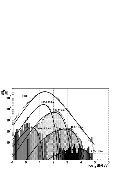
Figure 4: Final muon energy spectrum at constant transverse distance, $r$. Histograms show Monte Carlo results obtained with AIRES for $10^{19}$ eV proton showers at $80^{\circ}$ zenith angle compared to our prediction for the spectrum indicated by the continuous lines. The parameters used for these results were $\kappa=0.8$, $\gamma=2.6$, $\rho kl=21.1$ GeV.

If we approximate the $p_{t}$ distribution by the parameterization given in Eq. 2 the spectrum at a given $r$ is given by

$$\frac{d^{2}N}{dE_{i}dr}[z] = \frac{AB}{l}N_{0}\left(\frac{r}{l}\right)^{\lambda}\left[1-\frac{r^{2}}{l^{2}}\right]E_{i}^{-\gamma+\lambda+1}\left(\frac{E_{i}-\rho kl}{E_{i}}\right)^{\kappa}\exp{\left(-\frac{E_{i}r}{lQc}\right)}\Theta(E_{i}-mc^{2}-\rho kl),$$ (10)

$$\frac{d^{2}N}{dE_{f}dr}[z] = \frac{AB}{l}N_{0}\left(\frac{r}{l}\right)^{\lambda}\left[1-\frac{r^{2}}{l^{2}}\right]\left(E_{f}+\rho kl\right)^{-\gamma+\lambda+1}\left(\frac{E_{f}}{E_{f}+\rho kl}\right)^{\kappa}\exp{\left(-\frac{(E_{f}+\rho kl)r}{lQc}\right)}\Theta(E_{f}-mc^{2}).$$ (11)

In Fig. 4 we show the energy spectrum at constant transverse distance, $r$, given by the above equation compared to Monte Carlo results obtained with AIRES for a $80^{\circ}$ shower. We have used the values of $\kappa$ and $\gamma$ obtained from theoretical considerations and we fit the value of $\rho kl$ to the overall energy distribution at ground. The best fit value corresponds to an energy loss of $\rho kl\sim 21.1$ GeV. An alternatively approach could be to fit the parameters $\kappa$ and $\gamma$ in Eq. 7 to the overall energy distribution from the Monte Carlo data and use them, as effective parameters to predict the energy distributions at fixed values of $r$. The results obtained are not critically dependent on the specific values of the parameters used nor on the form of the distributions used as inputs for the calculations. In fact it is well known that the energy loss parameter $k$ is not constant but increases logarithmically with the muon energy. By taking it as a fitted parameter we include this energy dependence in an effective way. An analogous procedure can be applied to get the correlations between other distributions, for instance the $p_{t}$ distributions for different $r$ which are shown in Fig. 3.

For high zenith angles the production distance distribution is sharply peaked and fixing $z$ to $z_{0}$ is a good approximation. In Fig. 4 the results have been obtained in this way. For low zenith angles this approximation is not justified. We can instead consider the above equations to apply for a given $z$ and integrate them over the $z$ distribution. For example the energy distribution at fixed $r$ becomes then

$$\frac{d^{2}N}{dE_{i}dr}=\int\frac{d^{2}N}{dE_{i}dr}[z]h(z)dz.$$ (12)

For close to vertical showers this method of performing the $z$ integral reproduces the results obtained with the simulations with much better accuracy.

A close look at the distributions shown in Fig. 4 reveals that the energy distributions become broader as the transverse distance $r$ decreases. This can be understood in terms of Eq. 11, which predicts in general three distinct regions for the energy spectrum.

1. For $E_{f}<\rho kl$ the behavior is dominated by the term corresponding to the muon decay probability, i.e. by decay and energy loss. The spectrum is close to a simple power law $dN/dE_{f}\sim E_{f}^{\kappa}$.

2. For $E_{f}>\rho kl$ the spectrum reflects both the energy and transverse momentum distributions respectively through the indices $\gamma$ and $\lambda$. The behavior of the energy spectrum is again close to a simple power law with a modified index which combines the two parameters, $dN/dE_{f}\sim E_{f}^{-\gamma+\lambda+1}$.

3. For $p_{t}>Q$ the exponential suppression assumed in the transverse momentum distribution appears as a cutoff in the energy spectrum. It is simple to show that the suppression takes place for energies $E_{f}>\frac{lQc}{r}$. The cutoff energy grows as $r$ decreases and this makes the distributions broader. This suppression affects the average muon energy at a given $r$ and is responsible for much of the well-known correlation between average energy and transverse position for the muons.

The three behaviors can be appreciated in the energy distributions for small $r$. For large $r$ however the cutoff in transverse momentum arises for a final muon energy $E_{f}<\rho kl$. These distributions display a direct transition from the $E^{\kappa}_{f}$ behavior to the suppression at the large energy limit. The second condition ($E_{f}>\rho kl$) takes place at energies which are suppressed and thus has little influence on the bulk of the spectrum. We can estimate the approximate distance $r_{c}$ above which this happens, by combining the first and third conditions to obtain $r>r_{c}\sim\displaystyle\frac{Qc}{\rho k}\sim 1000$ m. Only for $r$ below this scale the spectrum will display two slopes discussed above and a cutoff at higher energies. It is interesting to notice that $r_{c}$ is a transverse length scale which is approximately independent of zenith angle. It can be seen that this scale is also responsible for changes in quantities related to the muon energy in showers, for example the correlation between average muon energy and transverse distance.

III Time delay associated with muon propagation

The time distribution of the muon signal at ground level is important. To study this we will consider the delays associated with different mechanisms in muon propagation. We measure the time delays with respect to a plane front moving in the shower axis direction and traveling at the speed of light. According to the simplifications discussed in section II, the muon arrival time will be determined by a combination of two effects. First there is a simple geometric effect (geometrical delay), muons arriving at distance $r$ from the shower axis will take longer, because they travel a larger path than those arriving at $r=0$. In addition these muons, being of finite energy, are further delayed with respect to the reference front moving at the speed of light because they travel more slowly (kinematic delay). We can thus express the total time delay as a sum of these two delays

$$t=t_{g}+t_{\epsilon}.$$ (13)

Here $t_{g}$ is the geometrical delay and $t_{\epsilon}$ is the kinematic delay.

The distribution of arrival times taking into account both the geometrical and the kinematic delays can be now obtained by taking a convolution of the distributions associated with the two effects

$$\frac{1}{N_{r}}\frac{d^{2}N}{dtdr}=g(t)\otimes\varepsilon(t)=\int g(t-t^{\prime})\varepsilon(t^{\prime})dt^{\prime},$$ (14)

where $g(t)$ and $\varepsilon(t)$ are the arrival time distributions due to the geometrical and kinematical delays respectively, both normalized to 1 and $N_{r}$ is a shorthand notation for $dN/dr$ which is needed for this normalization. We now study the two delays separately.

III.1 Geometrical delay

For high energy muons we can neglect, in a first approximation, the time delay associated with the finite muon energy. In that case we would simply convert the path length difference to a corresponding time delay. For a vertical shower we obtain

$$t_{g}=\frac{1}{c}\left(\sqrt{z^{2}+r^{2}}-z\right).$$ (15)

This relation implies that the delay of muons arriving at a given point on the ground, at a fixed transverse distance $r$, is only a function of the production altitude. The arrival time distribution of the muon signal can be obtained as

$$g(t)\equiv-\frac{1}{N_{r}}\frac{d^{2}N}{dtdr}=-\frac{dz}{dt}\frac{1}{N_{r}}\frac{d^{2}N}{drdz}=-h(z)\frac{dz}{dt}\frac{1}{N_{r}}\int dE_{i}\frac{d^{2}N}{dE_{i}dr}[z],$$ (16)

where $h(z)$, $d^{2}N/dE_{i}dr[z]$ (given in Eq. 10) and $dz/dt$ are functions of $z$ and therefore implicit functions of $t$ through Eq. 15 . It can be shown that the $z$ dependence of the integral of Eq. 10 over $E_{i}$ is $l^{1-\gamma}~{}[1-r^{2}/l^{2}]$. The first factor corresponds to an attenuation of the number of muons through decay Lorenzo_icrc and besides the normalization has little importance for very inclined showers. Moreover since the distance distributions obtained with AIRES only account for the muons that reach ground level, it can be argued that the fit takes care of it. As a result the functional form of $g(t)$ is given in implicit form through

$$g(t)\propto-h(z)\frac{dz}{dt}\left[1-\frac{r^{2}}{l^{2}}\right]$$ (17)

where for large zenith angles the last factor can be dropped.

It is relatively easy to understand that for inclined showers the geometrical effect implies that there is an asymmetry in the arrival times. The different path lengths traveled by the muons for different polar angles in the transverse plane ($\zeta$) (see Fig. 1) induce different delays. We can take this into account by changing the relation between $z$ and $r$ of Eq. 15 to include the excess path traveled by muons at different angles

$$t_{g}(z-\Delta)=\frac{1}{c}\left(\sqrt{(z-\Delta)^{2}+r^{2}}-(z-\Delta)\right),$$ (18)

where $\Delta=r\cos\zeta\tan\theta$, and $t_{g}$ is measured with respect to the shower front plane. Now we still use Eq. 16 to get the time distribution but $dz/dt$ must be obtained from Eq 18. Alternatively we can make the shift $z\rightarrow z+\Delta$ in the argument of $h(z)$

$$g(t)=-\frac{1}{N_{r}}\frac{d^{2}N}{dtdr}\propto-h(z+\Delta)\frac{dz}{dt}\left[1-\frac{r^{2}}{l^{2}}\right],$$ (19)

and still use Eq. 15 for $dz/dt$. As in our convention $z$ is measured along the shower axis from ground to production point, a given $dz/dt$ from Eq. 15 must be associated with a production point which is shifted by $\Delta$ to ensure that distance to production corresponding to a point $(r,\zeta)$ is precisely $z$. The above equation introduces, in a simple way, important asymmetries in time distribution for constant $r$ but different $\zeta$ angles.

In Fig. 5 we show an example of the pulse shape obtained using the result of Eq. 19 compared to the results obtained using Monte Carlo simulation carried out with AIRES. The agreement is reasonably good although there are significative differences. The predicted signal has a faster onset, is somewhat broader and has a shorter tail which is suggestive of a delay underestimate. We will show below that all these effects can be mostly attributed to the sub–luminal muon velocity.

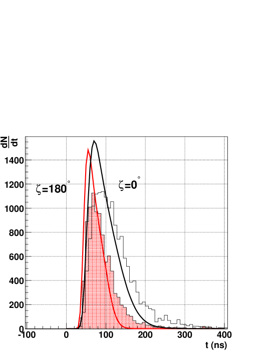
Figure 5: Arrival time distribution of muons at $r=$2000 m for a $10^{19}~{}$eV proton shower and incident zenith angle of $80^{\circ}$ obtained with AIRES, for two values of $\zeta=0,180^{\circ}$. The analytical result (continuous lines) with which it is compared takes into account only the geometrical delay. The observation altitude is 1400 m.

Once we have an expression for the time distribution we can obtain all relevant statistical quantities associated with it. For example the average arrival time at a fixed transverse distance is simply given by

$$<t(r)>=\int_{0}^{\infty}dt~{}\;t~{}\;g(t)=\int_{0}^{\infty}dz~{}\;h(z+\Delta)\;~{}t_{g}(z).$$ (20)

For example, for $r\ll z$, as is the case in inclined showers, we can expand $t_{g}$ given by Eq. 15, to get a simple expression relating the time delay and the transverse distance

$$<t(r)>=\frac{1}{2c}r^{2}\int_{0}^{\infty}\frac{dz}{z}h(z+\Delta).$$ (21)

For $h(z)$ we can use a log-Gaussian distribution centered at $z_{0}$ with a standard deviation $\sigma_{z}$, which is a good approximation for inclined showers (see Fig. 2)

$$h(z)=\frac{C}{z}\exp\left[-\frac{1}{2\sigma_{z}^{2}}(\log_{10}(z/z_{0}))^{2}\right],$$ (22)

where $C$ is a normalization constant. When we substitute the above distribution into the expression for the average geometric time delay we get the following analytical expression

$$<t(r)>=\frac{1}{2c}\frac{e^{-\sigma^{2}/2}\;r^{2}}{z_{0}-\Delta}.$$ (23)

where $\sigma=\ln(10)~{}\sigma_{z}$. The above expression gives the time curvature as obtained using the average arrival times of the signals as a function of the mean production depth. This curvature is directly related to the naive geometrical radius of curvature given by $1/2~{}r^{2}/z_{0}$. We notice that there is a correction factor (involving the width of the muon production function distribution) between the naive geometrical curvature and the time curvature.

We can also obtain the RMS value of the arrival time distribution of the muons at ground level as a function of $r$, $z_{0}$ and $\sigma$. The result is

$$\sigma_{t}(r)=\sqrt{<t^{2}>-<t>^{2}}=\frac{1}{2c}~{}\frac{r^{2}}{z_{0}-\Delta}\sqrt{1-e^{-\sigma^{2}}}\sim\frac{1}{2c}\frac{r^{2}}{z_{0}-\Delta}~{}\sigma.$$ (24)

This illustrates that the width of the arrival time distribution is proportional to the mean value, and hence it also rises as $r^{2}$ for a given shower. If $\sigma^{2}$ is small the proportionality factor becomes simply $\sigma$ as indicated in the last equality of the above equation.

In the same way we can obtained an estimation for the asymmetries in the geometric delay. We will define the asymmetry as

$$A=<t(r,\zeta=180^{\circ})>-<t(r,\zeta=0^{\circ})>$$ (25)

Then a simple calculation using the distributions introduced before shows that

$$A=\frac{r^{3}\tan\theta}{cz_{0}^{2}}e^{2\sigma^{2}}.$$ (26)

The asymmetry grows rapidly with $r$, as $r^{3}$. Also, notice that at fixed $r$ the average time can be approximated by a dipole type formula, $<t>=a+b\cos\zeta$.

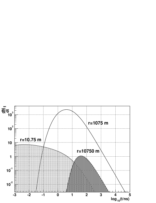
Figure 6: Kinematical delay distributions for $r\sim$ 10 m, 1 km, and 10 km obtained analytically. The parameters used are $\kappa=0.8$, $\lambda=1$, $Q=0.17$ GeV/c, and $\gamma=2.6$.

The main features of the arrival time distributions can be described with this simple model. As obtained in the above expressions, both the time delay and the width of the distribution grow as the transverse distance increases. The asymmetries obtained for different angles $\zeta$ are in agreement with the simulation results. It is interesting to notice that the arrival times for small polar angles ($\zeta\sim 0^{\circ}$), corresponding to the part of the shower front that touches ground earliest, are further delayed with respect to the late arriving part ($\zeta\sim 180^{\circ}$). We can expect different curvature corrections for different polar angles. The asymmetries are largest for intermediate zenith angles, according to this simple model. In the actual experimental situation, typically involving an array of particle detectors, the curvature of the front is sampled at different angles $\zeta$ so that systematic corrections to the arrival times and curvature of the front can be expected from this effect.

The results in Eq. 24 may be useful when considering the weight to be given to a given time in the reconstruction of the arrival direction. These results can be significantly improved by considering the delay time due to the muon velocity which we now describe.

A feature can be deduced from Eq. 19 which, in principle, opens up a new way to extract relevant information from the time structure of the shower front. It implies that a measurement of the arrival time of muons at a given distance to the core can give information on the production profile function of the muons. Important shower properties such as the shower maximum, which is related to the maximum in the muon production function, can in principle be obtained from it, to the extent that this approximation is valid.

III.2 Kinematic delay

There is an additional delay to be considered because muons with finite energy travel with a smaller velocity than that of light. This introduces the additional time delay $t_{\epsilon}$. For instance a 1 GeV muon traveling 40 km in vacuum would be delayed 750 ns with respect to the light front. In a medium such as air, muons have continuous energy loses and these delays are more complex to estimate. For this reason we have modeled the energy distributions in Section II-B, taking into account energy losses and muon decay.

Neglecting multiple scattering and magnetic effects, muons travel a distance $l=\sqrt{z^{\prime 2}+r^{2}}$ from production to ground level, where $z^{\prime}=z-\Delta$. With these simplifications the extra travel time taken by a muon of velocity $\beta c$ with respect to a photon is simply given by

$$t_{\epsilon}=\frac{1}{c}\int_{0}^{l}dl^{\prime}\left[\frac{1}{\beta(E)}-1\right].$$ (27)

We can substitute into the above equation the muon energy as a function of travel distance $l$ and then integrate. This can be done approximately using Eq. 4 to obtain

$$t_{\epsilon}=\frac{1}{c\rho k}\left(\sqrt{E_{i}^{2}-(mc^{2})^{2}}-\sqrt{E_{f}^{2}-(mc^{2})^{2}}\right)-\frac{l}{c},$$ (28)

where $E_{f}=E_{i}-\rho kl$ is the final muon energy when it reaches the ground. An interesting feature is revealed by this equation. It leads to the conclusion that there is a maximum time delay which is independent of $l$ and is approximately given by $mc^{2}/c\rho k\simeq 1.7~{}\mu$s. It corresponds to a muon that loses all its energy after traveling the distance $l$. This upper bound to the kinematic delay increases slightly if we consider an exponentially decaying density atmosphere.

If the final energy is much larger than the muon mass, $mc^{2}\ll E_{f}$ we can expand Eq. 28 to obtain

$$t_{\epsilon}\simeq\frac{1}{2}\frac{(mc^{2})^{2}}{c\rho k}\left[\frac{1}{E_{i}-\rho kl}-\frac{1}{E_{i}}\right].$$ (29)

When we take into account the muon energy spectrum, for instance in terms of production energy $E_{i}$, the arrival time distribution is then given by

$$\varepsilon(t_{\epsilon};z,r)\equiv-\displaystyle\frac{1}{N_{r}}\frac{d^{2}N}{dt_{\epsilon}dr}=-\frac{1}{N_{r}}\frac{d^{2}N}{dE_{i}dr}\frac{dE_{i}}{dt_{\epsilon}}.$$ (30)

At this stage, we make some simplifying assumptions to obtain simple expressions and discuss qualitative effects. If we expand Eq. 29 for muon energies that are large in relation to the energy loss in the atmosphere we obtain the following relation between time delay and muon energy

$$t_{\epsilon}\simeq\frac{1}{2}\frac{(mc^{2})^{2}l}{cE_{i}^{2}}.$$ (31)

If we now assume a fixed $p_{t}$ we can relate $E_{i}$ to $r$ to get

$$t_{\epsilon}\simeq\frac{1}{2}\frac{(mc^{2})^{2}}{cp_{t}^{2}}\frac{r^{2}}{z^{\prime}}$$ (32)

where we have expanded $l$ as a function of $z^{\prime}$ and $r$ for $r\ll z^{\prime}$. This is quite interesting because we obtain a kinematic delay which has a very similar expression to that obtained for the geometric time delay in Eq. 23. Very roughly one could expect an extra correction of order $m^{2}/p_{t}^{2}$ due to the kinematic delay. Assuming that the $p_{t}$ distribution is sharply peaked at about $170$ MeV/c this would result in $\sim 25\%$ more curvature. When the geometric delay is compared to simulation results, a systematic effect of this nature and of similar magnitude is indeed observed as remarked before. However the approximations involved to obtain this result are rather poor.

Fortunately we can obtain more reliable time distributions due to the kinematic delay through Eq. 30. We first invert Eq. 29 to get

$$E_{i}=\frac{\rho kl}{2}\left[1+\sqrt{1+\frac{t_{c}}{t}}\right],$$ (33)

Here $t_{c}$ is a characteristic time that involves energy loss and the atmospheric density

$$t_{c}=2\left(\displaystyle\frac{mc^{2}}{\rho k}\right)^{2}\displaystyle\frac{1}{c\,l}\simeq 500\;{\rm ns}\;\left[\frac{1\;{\rm km}}{l}\right].$$ (34)

We now have the ingredients to calculate the kinematic time delay distributions. We have only to substitute the time derivative and the muon energy and transverse distance distributions (for instance as obtained in Section II) into Eq. 30. The final result is cumbersome and we do not write it down explicitly.

As discussed in Section II-B the energy distributions have different behaviors depending on the transverse distance $r$ in relation to the critical radius $r_{c}$. We can consider the two cases separately to better understand the effect of the energy distribution on the time structure of the pulses. For $r\gg r_{c}$ we can simplify the energy distributions in Eq. 11 to a combination of a power law and an exponential. In that case the time distribution is simply

$$\varepsilon(t)\propto t^{-\kappa-2}\exp{\displaystyle\left(-\frac{1}{2}\frac{(mc^{2})^{2}r}{\rho klcQ}\frac{1}{ct}\right)}.$$ (35)

For $r\ll r_{c}$ the time structure is more complex because we obtain two different behaviors in the two regimes described. This can be seen through Eq. 33 in which the energy is regarded as a function of the delay time. The two regimes correspond to the times well below and well above $t_{c}$. These regimes also correspond to the limits $E_{f}\gg\rho kl$ and $E_{f}\ll\rho kl$ respectively. In these two limits the expressions for the energy in terms of $t$ can be simplified to

• for $t\ll t_{c}\;\;\;$ $E_{i}\simeq\sqrt{\displaystyle\frac{1}{2}\frac{(mc^{2})^{2}}{ct}l}$

• for $t\gg t_{c}\;\;\;$ $E_{f}\simeq\displaystyle\frac{1}{2}\frac{(mc^{2})^{2}}{\rho kct}$

When these relations are used together with the energy distributions to obtain the time distribution through Eq. 30 the two limiting behaviors obtained are

$$\varepsilon(t)\propto\left\{\begin{array}[]{ll}t^{-\kappa-2}&\textrm{if $t\gg t_{c}$}\\ \\ t^{\frac{\gamma-\lambda-4}{2}}\exp{\displaystyle\left(-\frac{1}{\sqrt{2lc}}\frac{mc^{2}r}{cQ}\frac{1}{\sqrt{t}}\right)}&\textrm{if $t\ll t_{c}$}\\ \end{array}\right.$$ (36)

Although we have made some effort to give analytical parameterizations where possible, making several approximations, we stress here that the complete procedure, without these approximations, can be implemented. Note that $r_{c}$ is below the distance separation between detectors in the Auger Observatory.

IV Results

Figure 7: Average time delay for muons injected at 10 km with a $\gamma=2.6$ spectrum. The lower curve shows the geometric delay. The dashed points show the kinematic delay. The upper curve is the sum of both.

We can combine the geometric and kinematic delays through the convolution given in Eq. 14. In Fig. 7 we show the average pulse time delay for the geometric and the kinematic delay times. We see that at small distances to the core the delay is dominated by the kinematic delay. This may seem surprising as near the core the characteristic muon energies are larger and one would expect a lower kinematic delay. However, near the core the spread on energy is larger (see Fig. 4) and the time delay is dominated by low energy muons.

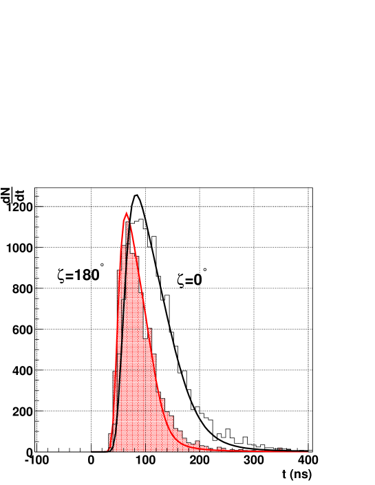
Figure 8: Example of arrival time distribution from Monte Carlo (histograms) for a $10^{19}$ eV proton shower and 80^∘ zenith angle compared to our analytical calculation. Muons arriving in the range $3.2<\log_{10}r<3.4$ ($r\sim$ 2000 m) are selected for two $\zeta$ angles in the transverse plane.

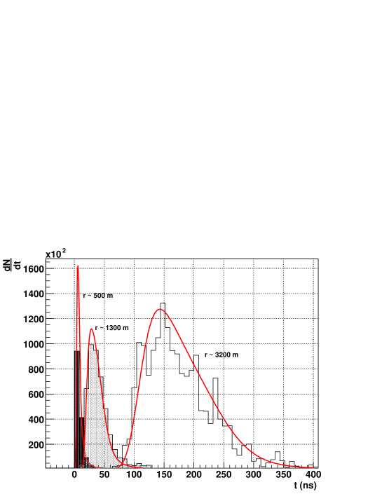
Figure 9: Example of arrival time distribution from Monte Carlo (histograms) for a $10^{19}$ eV proton shower and 60^∘ zenith angle and $\zeta=180^{\circ}$ compared to our analytical calculation. Muons arriving in the range $2.6<\log_{10}r<2.8$, $3.0<\log_{10}r<3.2$, $3.4<\log_{10}r<3.6$ as marked.

In Fig. 8 we show our analytical result for the arrival time distribution compared to the Monte Carlo. We can see that the agreement is very good both at low and large times. This is illustrated further in Fig. 9 where we show the time structure of muons arriving at transverse distances $r\sim$ 400 m, 1 km, and 2.5 km compared to the results obtained through direct simulation. These results have been obtained using $\kappa=0.8$ as suggested by theory, and $\lambda=1$, $\gamma=2.6$, $Q=0.17~{}$GeV/c and $\rho k$=0.2 GeV km^-1. Our results are encouraging and we can state that the main contributions to the time structure of muons in air showers have been identified and understood.

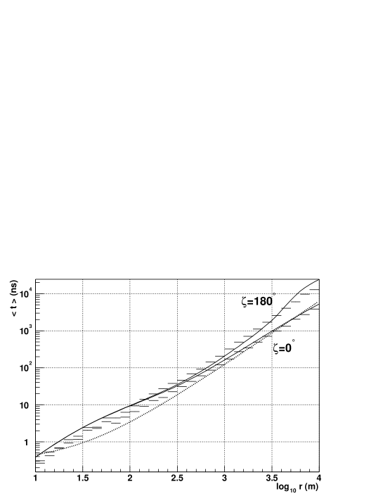
Figure 10: Average time delay as a function of transverse distance for two different positions in the transverse plane corresponding to $\zeta=0^{\circ}$ and $180^{\circ}$, as marked, for 10¹⁹ eV proton showers at zenith angle 60^∘. The histograms show the simulation results using AIRES and the lines show our analytical calculation. The lower (dotted)line shows the result of the phenomenological parameterization given in time1 .

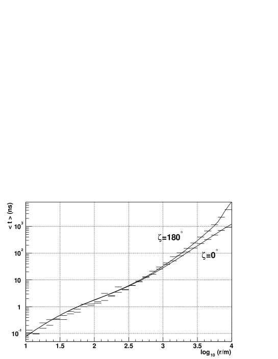
Figure 11: Same as Fig. 10 for $80^{\circ}$.

Figure 12: RMS values for the arrival time distributions of muons as a function of transverse distance for $10^{19}$ eV proton showers at zenith angle $60^{\circ}$ and for two different angles $\zeta$. The histograms show the simulation results using AIRES and the lines show our analytical calculation.

As an application of practical importance for direction reconstruction in extensive air showers we have calculated the average and the width of the arrival delay time distributions for different zenith angles as a function of distance to the shower axis, $r$. For near-vertical showers the production distance distribution can not be approximated by a delta function, as discussed at the end of Section II. The final kinematical delay distribution has been obtained by integrating the time delay corresponding to a given production distance $z$ over the $z$ distribution

$$\varepsilon(t;r)=\int h(z)\varepsilon(t;z,r)dz.$$ (37)

In Figs. 10, 11, 12, 13 we show the average and RMS values of the time distribution for times obtained with AIRES for 10¹⁹ eV proton showers and our analytical calculation for 60^∘ and 80^∘. It can be seen that the agreement is good specially the larger the zenith angle. The magnitude of the asymmetry is well reproduced as can be seen from the figure. For the RMS there are some discrepancies both at large and small distances. We believe that this is mainly an effect of fluctuations due to shower development and also due to the thinning procedure adapted in AIRES. In Fig. 10 we also show the parameterization given in Ref. time1 , based on a phenomenological formula suggested by Linsley Linsley .

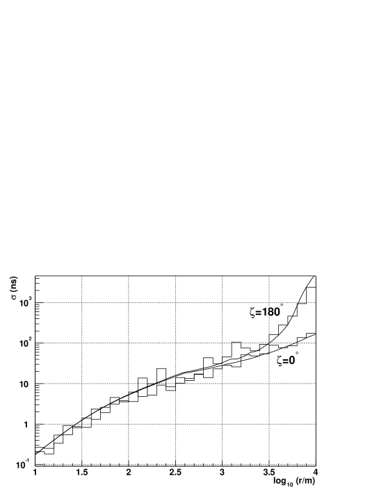
Figure 13: Same as Fig. 12 for $80^{\circ}$.

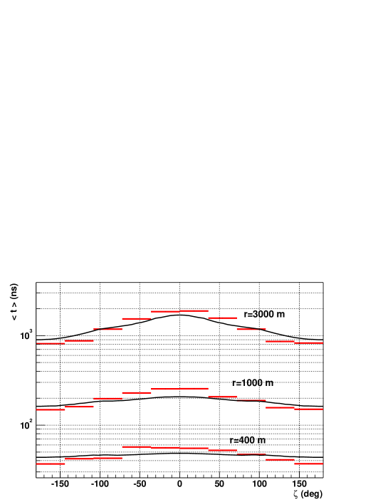
Figure 14: Asymmetry in the average time delay which is plotted as a function of the angle $\zeta$ in the transverse plane for 10¹⁹ eV proton showers at 60^∘ and fixed $r$ as marked. The histograms show the simulation results using AIRES and the lines show our analytical calculation.

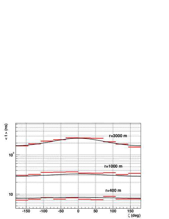
Figure 15: Same as Fig. 14 for zenith angle of $80^{\circ}$.

We have also calculated the asymmetries in the arrival time distributions. These can be approximated by a dipole correction to the average over $\zeta$ in the transverse plane. In Figs. 14, 15 we give the magnitude of the asymmetry as a function of $r$ for different zenith. The comparison between the analytical and the simulation results are given in a separate graph for characteristic distances.

We consider that an important application of this method will be to provide a description of the time distributions of muons in a given detector. Since the distributions used are continuous, at some point the number of muons that reach a given detector will have to be selected, and a sampling effect will arise because the finite number of muons that pass through a given detector. This sampling effect must be considered using the muon number distributions at ground level which have been discussed in detail in ref. ModelPaper .

Up to now the magnetic field has been ignored but it will affect the time structure of the signal in two ways. Firstly muon delays are modified because particles do not travel in straight lines. Secondly significant modifications of the time delays calculated so far are to be expected because the simple geometrical relation between $r$, $E_{i}$, $z$ and $p_{t}$ is known not to hold. The effect of the magnetic field on this relation is the basis of the model in ref. ModelPaper used to describe de density profiles of muons in inclined showers. There it is shown that the relative importance of the muon magnetic deflections with respect to deviations due to their $p_{t}$ is given by the parameter $\alpha=zB/p_{t}$. The condition of $\alpha>1$ corresponds to $\theta>80^{\circ}$ at the Auger site. Clearly when $\alpha\ll 1$ one can expect our description to be valid. We have also tested the validity of our description for angles corresponding to $\alpha>1$ at the Auger site. Contrary to what could be expected, magnetic effects do not appear to modify the shape of the time distributions in an important way for zenith angles below $84^{\circ}$. Therefore the results obtained in this article without the magnetic field are phenomenologically interesting also in the region $\alpha\sim 1$ and for the Auger site the range of application is zenith angles below $\sim 84^{\circ}$.

The model described here on its own has also ignored shower fluctuations. Nevertheless fluctuations of the arrival times of muons in an air shower can be related through the work presented here to fluctuations in the distributions discussed here. It is reasonable to assume that time fluctuations will be mostly due to the fluctuations in the longitudinal development of the shower and in the energy distribution of muons arriving at a given ground area.

V Summary and Conclusions

We have obtained a procedure that can be used to describe the time structure of the muon signal in extensive air showers. This procedure is based on two simple mechanisms, time delays due to the extra path length which are discussed as geometrical delays and those due to the sub-luminal velocity of the muons. The global delay can be expressed as a simple convolution of these two delays. The description combines the physical mechanisms with phenomenological descriptions of the energy, transverse momentum and position of the muons that are produced in an air shower with several approximations. The results obtained agree sufficiently well with those obtained with direct simulations for most distances of interest and for all zenith angles to be of a great importance for practical applications. This agreement allows us to state with some confidence that these two mechanisms dominate the time structure of the muons in air showers.

References

- (1) M. Nagano and A.A. Watson, Rev. Mod. Phys. 72, 689, (2000).
- (2) R. M. Baltrusaitis et al., Nucl. Instrum. Meth. A 240 (1985) 410.
- (3) M. Takeda [AGASA Collaboration], in Proceedings of the 26th International Cosmic Ray Conference (ICRC 99), Salt Lake City, Utah, 17-25 Aug 1999; N. Hayashida et al., Astrophys. J. 522, 225 (1999); M. Takeda et al. [AGASA Collaboration], Astropart. Phys. 19, 447 (2003).
- (4) T. Abu-Zayyad et al. [High Resolution Fly’s Eye Collaboration], arXiv:astro-ph/0208243; T. Abu-Zayyad et al., [High Resolution Fly’s Eye Collaboration], Astrophys. J. 557 (2001) 686.
- (5) The Pierre Auger Project Design Report, by Auger Collaboration, FERMILAB-PUB-96-024, Jan 1996; ( http://www.auger.org); Auger Coll., Properties and Performance of the Prototype Instrument for the Pierre Auger Observatory, submitted to Nucl. Instr. and Meth. A.
- (6) See Auger papers to be presented at the ICRC conference in Tokyo.
- (7) J. Lapikens, A. A. Watson, P. Wild and J. G. Wilson, in Int. cosmic Ray Conference, Denver, (1973), vol.4, p. 2582; J. Lapikens, J. Phys. A: Math. Gen. vol. 8 (1975) 838.
- (8) A.A. Watson and J.G. Wilson, J. Phys. A 7, 1119 (1974); R. Walker and A.A. Watson, J. Phys. G 7, 1297 (1981).
- (9) K. Honda et al., Phys. Rev. D 56 (1997) 3833.
- (10) G. Battistoni et al., Astropart. Phys. 9 (1998) 277.
- (11) T. Antoni et al. (Kascade coll.), Astropart. Phys. 18 (2003) 319.
- (12) A.M. Anokhina et al., Phys. Rev. D 60, 033004, (1999).
- (13) M. Ave, R.A. Vázquez, and E. Zas, Astropart. Phys. 14 (2000) 91.
- (14) L. Pentchev, P. Doll, and H.O. Klages, J. Phys. G: Nucl. Part. Phys. 25, 1235, (1999).
- (15) L. Pentchev and P. Doll, J. Phys. G: Nucl. Part. Phys. 27, 1459, (2001).
- (16) S.J. Sciutto, AIRES: A system for Air Shower Simulations, in Proc. og the XXVI Int. Cosmic Ray Conf., Salt Lake City (1999), vol. 1, p. 411; S.J. Sciutto, astro-ph/9911331.
- (17) Kalmykov N, Ostapchenko S, Pavlov A I, Nucl. Phys. B 52 (1997) 17.
- (18) L. Cazon et al., in Proc. of the XXVII Int. Cosmic Ray Conf., Hamburg, (2001), p. 1175.
- (19) J. Linsley, report 1983 (unpublished).