A Monte Carlo method to generate fluorescence light in extensive air showers

Abstract

A new approach to simulate fluorescence photons produced in extensive air showers is described. A Monte Carlo program based on CORSIKA produces the fluorescence photons for each charged particle in the development of the shower. This method results in a full three-dimensional simulation of the particles in a shower and of the fluorescence light generated in the atmosphere. The photons produced by this program are tracked down to a telescope and the simulation of a particular detector is applied. The differences between this method and one-dimensional approaches are quantitatively determined as a function of the distance between the telescope and the shower core. As a particular application, the maximum distance at which the Auger fluorescence telescope might be able to measure the lateral distribution of a shower is determined as a function of energy.

1 Introduction

There are several questions yet to be solved about cosmic rays with energy above $10^{18}\ eV$. The most exciting topics concern the existence of a cut off in the energy spectrum, the possible anisotropy of the sources, the chemical composition and the propagation mechanisms.

Particles with these energies arrive on Earth with a very low flux and therefore can only be studied by the detection of the extensive air showers (EAS) they produce in the atmosphere. The present HiRes [1] and the AGASA [2] experiments have contributed to our understanding of the nature of high energy cosmic rays and future detectors (Auger [3], EUSO [4], OWL [5] and Telescope Array [6]) are very promising due to the increase in collection area and the use of new technologies.

The fluorescence technique has been used successfully by the HiRes experiment and is also going to be used by the new generation of detectors: Auger, EUSO, Telescope Array and OWL. Fluorescence detectors measure the EAS by counting, as a function of depth, the photons produced by the excitation of nitrogen molecules due to the passage of the charged particles in the shower. The determination of the longitudinal profile and the time the photons have hit the detector allow the reconstruction of the energy and direction of the primary particle.

Monte Carlo simulations have been widely used by cosmic ray physicists to optimize their detectors and to determine reconstruction methods. One of the most popular and tested programs known in the cosmic ray community is CORSIKA [7]. CORSIKA simulates the development of the particles in a shower in a high level of sophistication including three-dimensional particle transport, electromagnetic interactions, decay of unstable particles, multiple scattering, deflection in the Earth’s magnetic field and several high energy hadronic interaction models. Comparisons of CORSIKA simulations and experimental data can be found in [8].

A shower with energy $10^{19}\ eV$ has more than $10^{10}$ particles and a Monte Carlo simulation would take a long time to follow all of them. Hillas [9] has overcome this problem by using a thinning algorithm in Monte Carlo simulations. This procedure follows only a fraction of the particles with energy below a certain limit and conserve the total energy in the shower. The use of this method has reduced the computational time to practical limits without decreasing significantly the quality of the simulations.

In contrast to the simulation of particles in a shower, the simulation of the fluorescence light produced by the passage of these particles in the air has been done with almost no detail. Calculations made so far were done based on one-dimensional simulations of the fluorescence photons following an average function given by a Gaisser-Hillas [10] profile. Apparently, the crude treatment given to the simulation of the fluorescence component was justified by the optics and electronics of the present generation of telescopes. However, for the future detectors this justification is certainly not going to be valid.

In reference [11], Sommers has made analytic calculations to show the possibility of detecting the lateral distribution of a shower with a fluorescence detector. His ideas have been exploited by Góra et al. [12] using simulations based on a Gaisser-Hillas longitudinal profile and a NKG [13, 14] lateral distribution function.

More recently, other groups have announced new fast simulations in development [15, 16] which may be used to produce fluorescence photons. These programs are based on a combination of numerical and Monte Carlo approaches and special attention must be taken in order not to reduce the intrinsic shower fluctuations.

The work presented here explains how we generate fluorescence photons in the CORSIKA framework. Our approach allows the simulation of this component of the shower with great detail. For each charged particle produced in the shower development, the corresponding fluorescence light is produced from the ionization energy loss and the are tracked to the detectors. Atmospheric attenuation may be applied and the particles continue to be followed by CORSIKA down to the observational level resulting in a full hybrid (fluorescence + particles) simulation. In particular, this simulation can be useful for the Auger Collaboration due to its hybrid design.

The atmospheric attenuation is done by a simple implementation that simulates the extinction of photons according to particular atmospheric properties. The user is allowed to implement different atmospheric extinction coefficients. Excluding the showers simulated in section 3.1 where no attenuations has been applied, all simulations in this paper were done with a midlatitude US Standard Atmosphere and scattering of light by aerosols and molecules was taken into account. The aerosol horizontal attenuation length and vertical scale height were set to $12\ km$ and $1.2\ km$, respectively. The mean free path for Rayleigh scattering was set to $2974\ g/cm^{2}$. Scattering of the fluorescence photons is not simulated in the present version which could be an important effect for some specific geometries of detection and therefore should be accounted for in future implementations.

Historically, the main advantage of using Monte Carlo simulations comparing to analytic models has been considered to be the possibility to reproduce the event by event fluctuations. Nevertheless, the development of the softwares has extended the differences beyond that, among which, we stress the possibility to inject almost all kind of primary particles, the detailed description of the atmosphere and the treatment of each shower component (hadronic and electromagnetic) in an independent way with parameters updated from the accelerator experiments.

Besides that, the simulation we has developed have some other improvements if compared to analytic or one-dimensional models regarding the fluorescence photons production. In a deeper level of analysis, the approach we present here is able to simulate the particle by particle fluctuation in the production of the fluorescence photons, since each charged particles is treated independently.

Moreover, the time information is available for each single photon taking into account its exact position in the atmosphere. This feature would allow for the first time a detailed study of the snapshots proposed in [11] with a good raytracing resolution.

Recently proposed experiments [17, 18] are planning to measure the fluorescence yield in more details than done so far by Kakimoto et al. [19]. The fluorescence yield varies with the particle energy and may be completely different for each particle type. The simulation presented here can easily take into account the dependencies of the yield as a function of energy and particle type for each particle in the shower after they have been measured by the proposed experiments. This great level of detail would be practically impossible to be accounted for in a analytical model or in an one-dimensional Gaisser-Hillas approach.

In this paper, we describe the simulation, test it against old and simple approximations and illustrate the use of the program by calculating the lateral size of the shower as a function of the distance to a ground based telescope. This application shows that the lateral distribution of showers with energies $10^{18}$, $10^{19}$ and $10^{20}\ eV$ measured by detectors similar to the Auger telescopes configuration can not be neglected when distances from the detector to the shower axis are shorter than $4\ km$, $8\ km$ and $14\ km$, respectively.

2 Fluorescence Light Simulation

We used CORSIKA as the basic framework for the generation of particles in the shower. The detailed simulation implemented in CORSIKA makes all the information needed to generate fluorescence photons for every charged particle in a shower available. Explicitly, the position of creation and death of the current particle and the energy deposit of this particle in the atmosphere are accessible.

For each charged particle produced inside CORSIKA, a new subroutine that generates the fluorescence light is called. With the initial and final positions $(\vec{r}_{i},\vec{r}_{f})$ and energies $(E_{i},E_{f})$ of the particle the subroutine does a Monte Carlo simulation for the production and propagation of fluorescence photons.

However, when the energy of a particle falls below a certain value, it is neglected by CORSIKA and the information needed to create fluorescence photons is not available. For electrons and positrons below the energy cut, $50\ keV$, we made the hypothesis that they deposit all the available energy as they are discarded by CORSIKA. We also assume that the track length traveled by these particles ($\Delta X$) is given by the Bethe-Bloch theory and the stopping range is calculated assuming the continuous-slowing-down-approximation.

As explained previously, in simulations of high energy EAS one usually adopts a thinning method in order to reduce the number of particles to be followed and stored. In this procedure a weight W is attributed to each particle. As can be seen in Figure 1, where we show the average weight of particles in a $10^{19}\ eV$ shower simulated with thinning factor $10^{-6}$, many particles have weight well beyond 1000.

In order to avoid the necessity of applying an unthinning procedure in the detector simulation we considered the energy deposited by a single particle as given by: $\Delta E=W\cdot\Delta E^{single}_{particle}$.

Since the total path ($\Delta X$) and the energy deposited by particles ($\Delta E$) with energy above the energy cuts and by electrons and positrons with energy below the cutoff are now known, the number of photons produced by each of these particles can be calculated using the fluorescence yield given by Kakimoto et al. [19]:

$$N_{pht}=\int\frac{dE}{dX}\;\rho\;dx\left(\frac{A_{1}}{1+\rho B_{1}\sqrt{T}}+\frac{A_{2}}{1+\rho B_{2}\sqrt{T}}\right)\left(\frac{dE}{dX}\right)_{1.4\ MeV}^{-1}$$ (1)

where the temperature $T$ and the density $\rho$ are functions of the altitude and the constants are $A_{1}=89.0\ m^{2}kg^{-1}$, $A_{2}=55.0\ m^{2}kg^{-1}$, $B_{1}=1.8\ m^{3}kg^{-1}K^{-1/2}$, $B_{2}=6.5\ m^{3}kg^{-1}K^{-1/2}$ and $(dE/dX)_{1.4\ MeV}=1.8\ MeV/(g/cm^{2})$.

Finally, since fluorescence emission is isotropic, only a small fraction of these photons is emitted towards the detectors and this fraction depends only on the distance to the detector and on its geometry. Once the user has defined the position and radius of the detectors for which the simulation is done, the average number of photons emitted by a charged particle in the direction of the detectors can be calculated as:

$$\overline{\aleph}=N_{pht}\cdot\frac{d\Omega_{tot}}{4\pi}$$ (2)

where $d\Omega_{tot}$ is the solid angle subtended by all the detectors.

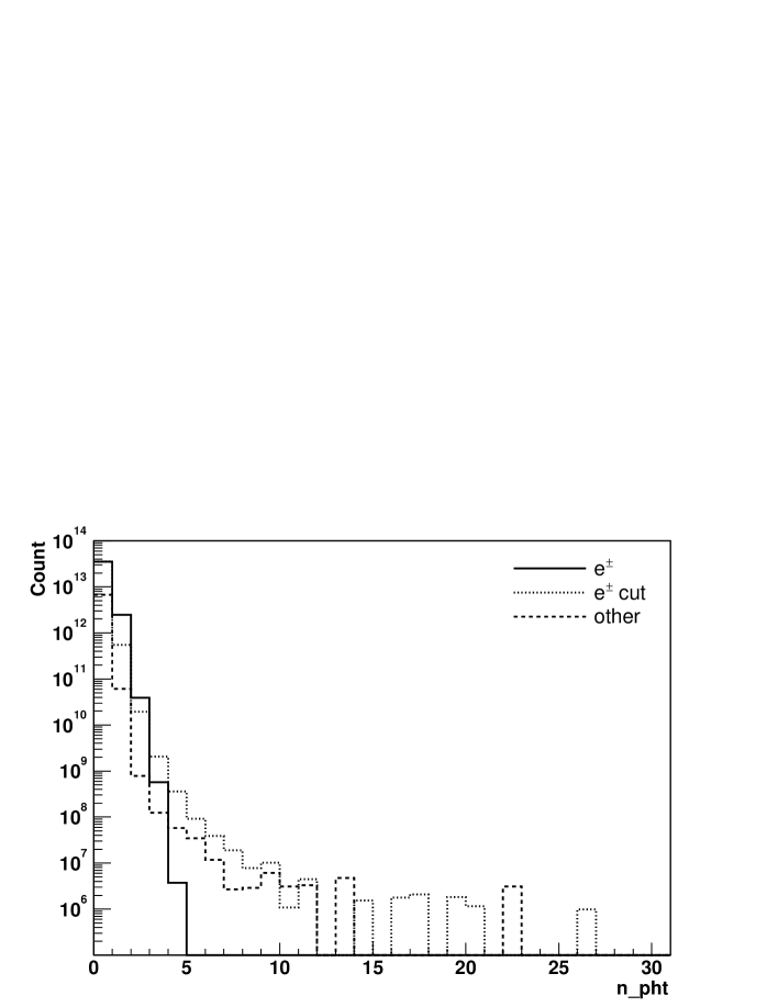
Figure 2: Distribution of the number of photons emitted by a single particle toward the telescopes. Same events as in figure 1. The telescope was positioned $15\ km$ away from the shower core.

In general, we have $\overline{\aleph}<1$ because the solid angle subtended by the detectors is small compared to $4\pi$ and despite the great amount of photons emitted, the probability that any of them will be directed inside $d\Omega_{tot}$ is very small. According to the physical process involved, the final number of photons (N) emitted towards the detectors, by the passage of one given particle, can be described by a Poisson distribution with average $\overline{\aleph}$. Figure 2 shows the distribution of the number of photons emitted towards the detector, for the same events as in figure 1.

Knowing the number of photons to be emitted by the particle, its trajectory is divided in N equal intervals and one photon is emitted from the center of each interval. The emission point is set to the middle of each interval and the direction of emission of the photon is drawn inside the solid angle of one of the detectors. Therefore, we can evaluate whether or not the photon’s trajectory lies within the solid angle subtended by the disk that defines the detector. If the intersection of the trajectory with the disk exists, the emission position, propagation direction, time and wavelength of photons that hit a detector are saved in a file. The wavelength is drawn from the known fluorescence spectrum [20].

3 Tests

The longitudinal profile of charged particles is the most important feature of a cosmic ray shower measured by fluorescence detectors. The longitudinal development of the shower is used to estimate the energy and gives a hint on the mass of the primary particle.

In order to test the fluorescence photon production we have compared the number of photons produced along the shower development and the arrival time of these photons at a telescope simulated by our program with an analytic calculation based on the longitudinal energy deposited in the atmosphere as given by standard CORSIKA.

We have also compared the longitudinal profile of a real event detected by the Fly’s Eye telescope [21] with the simulation of the same shower.

3.1 Certification of the Number and Arrival Time of Photons

We have simulated vertical showers with energy $10^{18}\ eV$. For this application, electrons were chosen as primary particle of the showers because we would like to avoid confusions derived from the energy channeled into neutrinos, high energy muons and nuclear excitation in hadronic showers [22]. The thinning factor was set to $10^{-6}$ to reduce fluctuations in the longitudinal profile and no atmospheric attenuation was applied.

The fluorescence photons produced by our code are propagated down to a telescope of radius $10\ m$, positioned $40\ km$ away from the shower core. For the studies presented in this section, we have stored the height of production and the arrival time of the photons detected by the telescope as can be seen in figures 4 and 3.

The standard version of CORSIKA records the energy deposited in the atmosphere by all particles in intervals of a given grammage. We have set the bin size to be 10 $g/cm^{2}$ and from the longitudinal energy deposit profile we were able to calculate analytically the number of photons produced in a bin and consequently the average arrival time of this photons in the telescope.

To the amount of energy deposited in one bin corresponds a certain amount of photons detected in the telescope that is given by equations 1 and 2 where density and temperature can be approximated to the values at the middle of the bin. Since the distance between the telescope and the middle of the bin along the axis of the shower is known we can also calculate the time these photons would hit the detector.

In this calculation all particles are considered to be emitted along the axis of the shower so that to be able to compare with our three-dimensional program we have positioned the telescope far away of the axis ($40\ km$) in order to minimize the differences. However, the number of photons measured by a regular fluorescence detector with few meters of aperture would be very small at this distance. To avoid fluctuations due to low statistics we simulated a detector with $10\ m$ of aperture. No telescope optics or electronics were simulated.

Figure 4 shows, for a single shower, the longitudinal profile of photons that end up to be detected in the telescope and the results of the analytic calculation based on the energy deposited in the atmosphere. The agreement between our simulation and the simple calculations is perfect. Similar results are obtained for all showers at different energies and inclinations.

Figure 3 shows the arrival time in bins of 100 ns as given by our program and the analytic calculation. Again the agreement is very good and similar results are obtained for all showers at different energies and inclinations.

The comparisons shown in these graphics proves that our simulation program is able to reproduce the right number and arrival time of photons at the telescope as expected by simple arguments.

3.2 Comparison to a Real Event

In 1995, the Fly’s Eye experiment detected a very clear shower with energy well beyond the GZK cut-off. This event has been published [21] and we used the reconstructed longitudinal profile as a test of the consistency for our program.

The famous shower has landed $13.6\ km$ away from the telescope and its primary energy and zenith angle were estimated as $320\ EeV$ and $43.9^{o}$, respectively. See [21] for details of the reconstruction. We have simulated with our program 10 events with the same energy and geometry of the Fly’s Eye shower: 5 initiated by proton, and 5 by iron. The produced photons were propagated through the optics of a telescope similar to the Auger Fluorescence Telescopes [3]. The design of these telescopes is a Schmidt camera with a corrector ring determining an aperture of radius $1.1\ m$ and a spherical mirror with $30^{o}\times 30^{o}$ field of view [23]. The photomultiplier camera is formed by 440 phototubes in a grid of $22\times 20$ with $1.5^{o}$ field of view each. In the simulations of the signal detected by the photomultipliers we have added a poissonian noise with average equal to the night sky background.

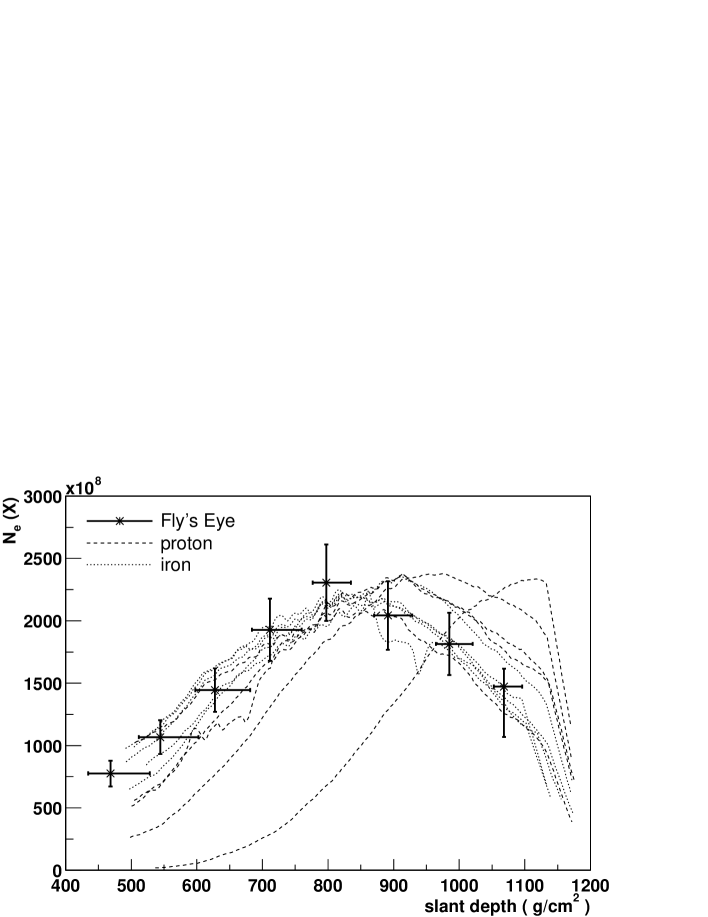
Figure 5: Comparison of the longitudinal profiles of five proton and five iron showers simulated by our code to the profile reconstructed by the Fly’s Eye Collaboration.

The simulation was reconstructed to give the longitudinal profile according to the standard procedure described in [21]. Figure 5 shows a comparison of the longitudinal profile determined by the Fly’s Eye group with the longitudinal profile simulated with our code. An integration of the profile leads to the energy of the primary particle. The estimated energy from the simulations is $3.4\pm.51(rms)\times 10^{20}\ eV$ which is in good agreement with the value estimated by the Fly’s Eye Collaboration.

4 Applications

Several new applications are possible with this three dimensional fluorescence and particle simulation. Among them, we could stress the verification of hybrid reconstruction methods, the analysis of arrival time of the photons in a telescope as suggested by Sommers [11], the determination of the “missing energy” [22] in a shower and the configuration of the new generation of fluorescence detectors.

However, the first demanding application is to determine the capability of a fluorescence detector to distinguish a one-dimensional shower from a three-dimensional one. In other words, in which conditions a fluorescence detector is going to detect the lateral distribution of particles in a shower?

To answer this question, we have simulated two sets of 100 vertical showers initiated by $10^{19}\ eV$ protons. The thinning factor was set to $10^{-6}$. One set was simulated with the three-dimensional program described here, and the other with an one-dimensional simulation following a Gaisser-Hillas distribution. Ten telescopes were positioned in a line from $2\ km$ up to $20\ km$ away from the core of the shower, equally spaced in steps of $2\ km$.

We have simulated the fluorescence detectors used by the Auger collaboration described in section 3.2 and the quantitative conclusions shown here might be very different for detectors with different configurations, in particular for telescopes with different pixel size.

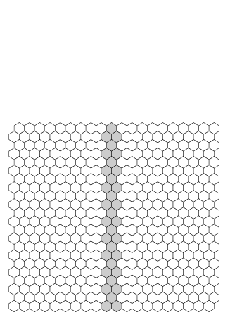
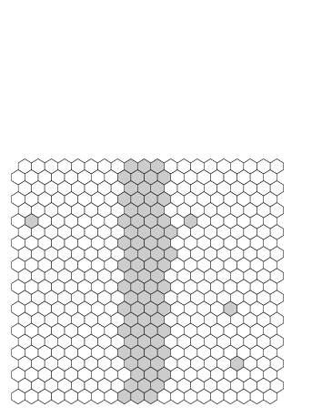
Figure 6: Distribution of the triggered pixels on the camera of a telescope positioned $4\ km$ from the shower axis. The results of the one-dimensional and three-dimensional simulations of the shower are shown in the left and right panels, respectively.

Figure 6 shows an example of the number of pixels triggered in the camera by one-dimensional and three-dimensional methods for a shower falling $4\ km$ far from the telescope. Adopting a simple trigger condition given by those pixels with signal 4$\sigma$ above the average of the noise in that event, we are able to measure the number of pixels triggered in the Auger telescopes as a function of the distance of the shower core for one-dimensional showers and for three-dimensional showers. Figure 7 shows this comparison. The number of pixels triggered by the shower simulated with the one and three-dimensional approaches are, within the statistical variation, the same for distances greater than $8\ km$.

Another parameter that can give us the sensitivity of the detector to the lateral distribution of showers is the radius of a circle ($\zeta$ measured in degrees) on the photomultiplier camera which maximizes the signal to noise ratio, $S/N$. The distribution of the triggered pixels in a camera allows us to determine the main track of the shower. The method to determine $\zeta$ consists in searching the radius of the circle centered on the track along the entire path which maximizes $S/N$.

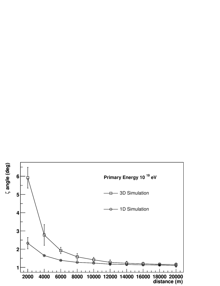
Figure 8: The $\zeta$ angle as function of the distance from the core to the telescope for one and three-dimensional simulations of showers with primary energy of $10^{19}\ eV$.

Figure 8 shows the curve of $\zeta$ obtained for one and three-dimensional simulations as a function of the distance between the telescope and the core position of the shower. The $\zeta$ angle increases for small distances for the one-dimensional simulations because of the scattered Čerenkov light included in the simulations.

Figure 8 shows that for core distances closer than $8\ km$ of the telescope the lateral distribution of the particles in the shower produces a measurable spread of the signal in the photomultiplier camera. The $\zeta$ angle increases quickly as the core gets closer to the telescope.

4.1 Energy Dependency

The capability of a fluorescence telescope to distinguish between one-dimensional and three-dimensional showers certainly depends on the primary energy of the shower. With increasing energy, the lateral spread of the particles gets larger in comparison with one-dimensional approximations and it should be easier to measure the width of the signal.

In order to study the energy dependency we simulated 50 vertical proton showers with primary energy $10^{18}\ eV$ and 10 vertical proton showers with primary energy $10^{20}\ eV$. The number of events was reduced in comparison to the previous analysis because the errors had shown to be small. We used the same thinning factor set to $10^{-6}$.

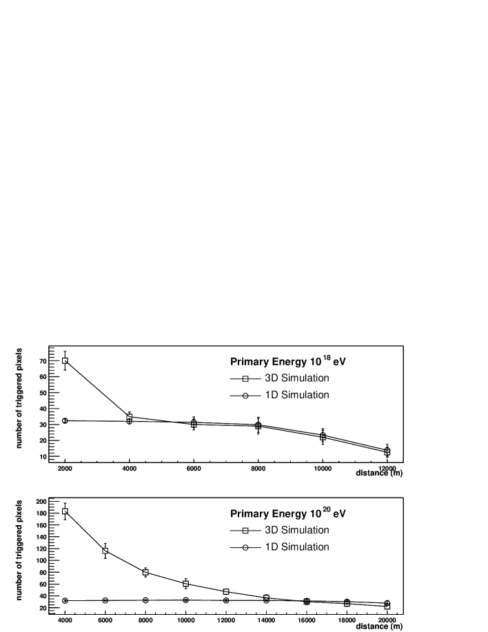
Figure 9: The number of triggered pixels as function of the distance from the core to the telescope for one and three-dimensional simulations of shower with primary energy of $10^{18}\ eV$ and $10^{20}\ eV$.

Figure 9 shows the number of pixels triggered as a function of the distance from the shower axis. We show the comparison between one-dimensional and three-dimensional simulations. Similar plots for the $\zeta$ angle have been done and show the same results. We have limited the distance from the axis to the shower in the region we expected to find the separation between the one and three dimensional approaches. Based on figures 7 and 9 we are able to determine the maximum distance that a fluorescence telescope may be able to measure the lateral distribution of a shower as a function of energy as being $4\ km$ for $10^{18}\ eV$, $8\ km$ for $10^{19}\ eV$ and $14\ km$ for $10^{20}\ eV$ showers.

4.2 Evaluating the influence of the thinning

The distribution of weights given as a function of the lateral distribution of the shower is not constant and depends on the particle type. Therefore, the unthinning procedure for the production of fluorescence photons proposed in section 2 should be tested in order to guarantee that no spurious fluctuations have been introduced in the determination of the lateral size of the shower seen by a fluorescence telescope.

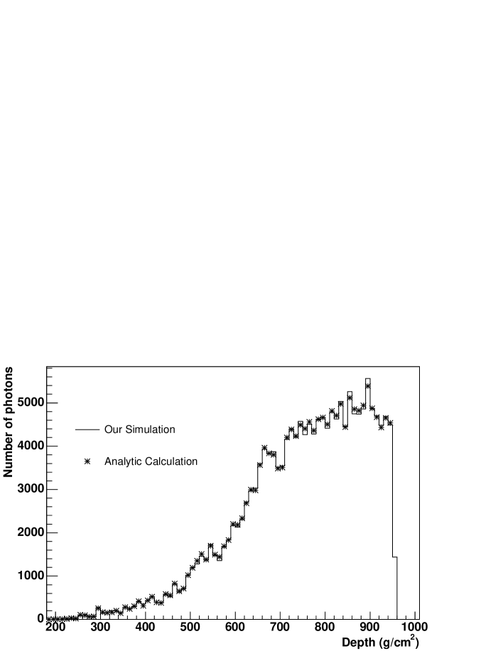
Figure 10: Comparison between the number of photons as a function of atmospheric depth calculated from the longitudinal energy deposited in the atmosphere and simulated by our program. The thinning factor as set to $10^{-4}$.

Figure 10 shows that the unthinning procedure implemented here is not able to smooth the fluctuations in the longitudinal profiles. In this figure, we show the number of photons detected by the telescope as a function of depth for one vertical shower initiated by an electron with energy $10^{18}\ eV$. The thinning factor was set to $10^{-4}$. The telescope is $40\ km$ away from the axis of the shower and has $10\ m$ radius. We have set the same configuration of the shower presented in figure 4 except for the thinning factor. The analytic calculations were carried out in the same way as explained in section 3.1.

The comparison between figure 4 (Thinning Factor $10^{-6}$) and figure 10 (Thinning Factor $10^{-4}$) illustrates the fluctuations caused by a strong shower thinning. Nevertheless, figure 10 shows our simulation produces the expected number of photons independently of that factor.

However, in this article we would like to guarantee that the results shown in section 4 are independent of the thinning factor. Therefore, we have also used the number of pixels triggered in the camera and the $\zeta$ angle to verify the thinning influence on the final measurement of the lateral spread of the showers. We have simulated ten vertical proton initiated showers with energy $10^{19}\ eV$ for different thinning factors ($10^{-4}$,$10^{-5}$, $10^{-6}$ and $10^{-7}$) through the Auger telescopes and determined the distribution of the number of pixels triggered and $\zeta$ as described above.

Table 1 shows the average number of pixels triggered and $\zeta$ angle for each thinning factor for telescopes at $4\ km$ and $8\ km$ away from the shower axis. As can be seen, the unthinning algorithm does not introduce any detectable fluctuation in the shower lateral size measured by Auger type telescopes for the thinning factor ranging from $10^{-4}$ to $10^{-7}$.

5 Conclusions

We have presented here a new approach to simulate fluorescence photons in an atmospheric air shower. A three-dimensional and fully hybrid (particles+photons) simulation tool was developed under the CORSIKA framework. In our routines, fluorescence photons were produced for all charged particles in a shower and for electrons and positrons with energy below the CORSIKA cut-off.

This program is going to be useful for the new generation of detectors (Auger, EUSO, Telescope Array and OWL) due to the improvement in the technology used by them. As shown here, for the new observatories the shower can not be considered one-dimensional in all cases and therefore a three-dimensional approach should be used to optimize the construction and in the elaboration of reconstruction methods.

In this paper, the number of photons produced along the longitudinal development of the shower and the arrival time of the photons in the detector determined by our program have been compared to analytical calculations based on the energy deposited profile given by CORSIKA.

A good agreement can be seen in figures 4 and 3. The famous $320\ EeV$ shower detected by the Fly’s Eye experiment was also simulated according to the geometry given in [21]. The consistency of our simulation can be seen as a test of the approach proposed here from one hand and as confirmation of the profile reconstructed by them from the other hand.

Our code was approved in several comparisons of simulated and real data. The arrival time, the longitudinal profile and the energy determined by our simulation show a very good agreement to what has been published so far.

The fluctuation due to thinning algorithm introduced in section 2 has been tested in respect to its influence on the lateral distribution of particles. No effect of the thinning was found in a range from $10^{-4}$ to $10^{-7}$ of the thinning factor when detectors similar to the Auger telescopes configuration are used.

Applications of the code were performed. We determined the sensitivity of a fluorescence telescope of the kind used by the Auger collaboration to the lateral distribution of the particles in a shower. Such a telescope could distinguish a real shower from a one dimensional approximation for distances of the core closer than $4\ km$ for $10^{18}\ eV$ showers, $8\ km$ for $10^{19}\ eV$ showers and $14\ km$ for $10^{20}\ eV$ showers.

These results represent a limit on the possibility to measure the lateral distribution of particles with a fluorescence telescope based on time information as suggested by [11]. However, a great number of showers with energy beyond $10^{19}\ eV$ with core closer $8\ km$ can be detected and reconstructed by the present and future fluorescence telescopes. For this subset of events we suggest a detailed analysis of the data in order to possibly measure the lateral distribution of the particles.

6 Acknowledgments

The authors would like to thank Dieter Heck for very fruitful discussions during the development of this code. This work was supported by the Brazilian population via the science foundations FAPESP and CAPES to which we are grateful. The calculations were done at Campinas using the computational facilities funded by FAPESP. We are also very grateful to Carlos Escobar for reading the manuscript and for useful discussions.

Thinn. Factor	$\zeta$ Angle (deg)		N Pixels Trigg.
	$4\ km$	$8\ km$	$4\ km$	$8\ km$
$10^{-4}$	2.4$\pm$0.87	1.5$\pm$0.1	87.7$\pm$3.1	35.3$\pm$3.9
$10^{-5}$	2.5$\pm$0.1	1.4$\pm$0.1	78.6$\pm$6.4	35.6$\pm$2.6
$10^{-6}$	2.4$\pm$0.06	1.4$\pm$0.1	82.0$\pm$4.5	35.5$\pm$2.3
$10^{-7}$	2.4$\pm$0.1	1.4$\pm$0.1	76.3$\pm$4.5	36.0$\pm$2.4

Table 1: Number of pixels triggered and $\zeta$ angle for different thinning factors and two telescopes at $4\ km$ and $8\ km$ away from the shower axis. The values are the average and standard deviation for a sample of ten vertical proton induced showers with energy $10^{19}\ eV$.

Figure 1: Mean distribution of weights for 10 proton showers of $10^{19}\ eV$ and zenith angle $45^{o}$. The thinning level was set to $10^{-6}$.

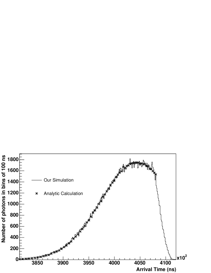
Figure 3: Comparison between the number of photons collected in bins of 100 ns in the detector as a function of time as simulated by our program and determined from analytic calculations. Time starts when first interaction happened.

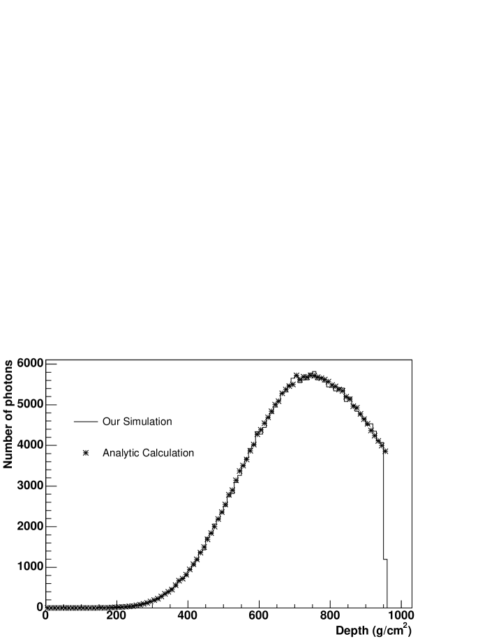
Figure 4: Comparison between the number of photons as a function of atmospheric depth calculated from the longitudinal energy deposited in the atmosphere and simulated by our program. The thinning factor as set to $10^{-6}$.

       

Figure 7: The number of triggered pixels as function of the distance from the core to the telescope for one and three-dimensional simulations of shower with primary energy of $10^{19}\ eV$.

References

- [1] T. Abu-Zayyad, et al., The prototype high-resolution fly’s eye cosmic ray detector, Nucl. Instr. Meth. A (450) (2000) 253.
- [2] M. Takeda, et al., Phys. Rev. Lett. 73 (1994) 3491.
- [3] The Auger Collaboration, Properties and perfomance of the prototype instrument for the Pierre Auger Observatory, Nuclear Instruments and Methods in Physics Research A, 523 (2004) 50-95.
- [4] M. Teshima, et al., EUSO (The Extreme Universe Space Observatory) - Scientific Objectives, in: T. Kajita, Y. Asaoka, A. Kawachi, Y. Matsubara, M. Sasaki (Eds.), Int. Cosmic Ray Conf., Universal Academy Press, Tsukuba, 2003, p. 1069.
- [5] P. Dierickx, et al., in: R. G. T. Andersen, A. Ardeberg (Ed.), Proceedings B ckaskog Workshop on Extremely Large Telescopes, 2000, p. 43.
- [6] Y. Arai, et al., The Telescope Array Experiment: an overview and physics aims, in: Int. Cosmic Ray Conference, 2003, p. 1025.
- [7] D. Heck, J. Knapp, J. Capdevielle, G. Schatz, T. Thouw, A Monte-Carlo code to simulate extensive air showers - report FZKA 6019, Tech. rep., Forschungszentrum Karlsruhe (1998).
- [8] M. Nagano, et al., Comparison of AGASA data with CORSIKA simulation, Astroparticle Physics 13 (2000) 277.
- [9] A. M. Hillas, Nucl. Phys. B (Proc. Suppl.) 52B (1997) 29.
- [10] T. K. Gaisser, A. M. Hillas, Reliability of the method of constant intensity cuts for reconstructing the average development of vertical showers, in: Int. Cosmic Ray Conf., Vol. 8, Plovdiv (Bulgaria), 1977, pp. 353–356.
- [11] P. Sommers, Capabilities of a giant hybrid air shower detector, Astroparticle Physics 3 (1995) 349–360.
- [12] D. Góra, P. Homola, M. Kutschera, J. Niemiec, B. Wilczynska, H. Wilczynski, Optical image of an extensive air shower, Astroparticle Physics.
- [13] A. A. Lagutin, A. V. Plyasheshnikov, V. V. Uchaikin, The radial distribution of electromagnetic cascade particles in the air, in: Int. Cosmic Ray Conf., Vol. 7, Kyoto (Japan), 1979, pp. 18–21.
- [14] J. N. Capdevielle for the KASCADE Collaboration, Local age parameter and size estimation in EAS, in: Int. Cosmic Ray Conf., Vol. 4, 1991, pp. 405–408.
- [15] H.-J. Drescher, G. Farrar, Phys. Rev. D 67 (2003) 116001.
- [16] J. Alvarez-Muniz, et al., Phys. Rev. D 66 (2002) 033011.
- [17] E. Kemp, et al., Study of the fluorescence yield for electrons between 0.5 - 2.2 mev, in: Proc. 28th Int. Cosmic Ray Conf., p. 853.
- [18] F. Arciprete, et al., AIRFLY: Air fluorescence induced by electrons in a wide energy range, in: Proc. 28th Int. Cosmic Ray Conf., p. 837.
- [19] F. Kakimoto, E. C. Loh, M. Nagano, H. Okuno, M. Teshima, S. Ueno, A measurement of the air fluorescence yield, Nucl. Instr. Meth. A (372) (1996) 527–533.
- [20] A. N. Bunner, Ph.D. thesis, Cornell University (1964).
- [21] D. J. Bird, et al., Detection of a cosmic ray with measured energy well beyond the expected spectral cutoff due to cosmic microwave radiation, Astrophysical Journal 441 (1995) 144–150.
- [22] C. Song, Z. Cao, B. R. Dawson, B. E. Fick, P. Sokolsky, X. Zhang, Energy estimation of UHE cosmic rays using the atmospheric fluorescence technique, Astropart. Phys. 14 (2000) 7.
- [23] M. A. L. de Oliveira, V. de Souza, H. C. Reis, R. Sato, Manufacturing the Schmidt corrector lens for the Pierre Auger Observatory, Nuclear Instruments and Methods in Physics Research A, 522 (2004) 360-370.