The Stellar Content of the Southern Tail of NGC 4038/9 and a Revised Distance

Abstract

We have used the Hubble Space Telescope and Wide Field Planetary Camera 2 to image the putative tidal dwarf galaxy located at the tip of the Southern tidal tail of NGC 4038/9, the Antennae. We resolve individual stars, and identify two stellar populations. Hundreds of massive stars are present, concentrated into tight OB associations on scales of $200$ pc, with ages ranging from $2$-$100$ Myr. An older stellar population is distributed roughly following the outer contours of the neutral hydrogen in the tidal tail; we associate these stars with material ejected from the outer disks of the two spirals. The older stellar population has a red giant branch tip at $I=26.5\pm 0.2$ from which we derive a distance modulus $(m-M)_{0}=30.7\pm 0.25$. The implied distance of $13.8\pm 1.7$ Mpc is significantly smaller than commonly quoted distances for NGC 4038/9. In contrast to the previously studied core of the merger, we find no super star clusters. One might conclude that SSCs require the higher pressures found in the central regions in order to form, while spontaneous star formation in the tail produces the kind of O-B star associations seen in dwarf irregular galaxies. The youngest population in the putative tidal dwarf has a total stellar mass of $\approx 2\times 10^{5}M_{\odot}$, while the old population has a stellar mass of $\approx 7\times 10^{7}\leavevmode\nobreak\ M_{\odot}$. If our smaller distance modulus is correct, it has far-reaching consequences for this proto-typical merger. Specifically, the luminous to dynamical mass limits for the tidal dwarf candidates are significantly less than $1$, the central super star clusters have sizes typical of galactic globular clusters rather than being $1.5$ times as large, and the unusually luminous X-ray population becomes both less luminous and less populous.

1. Introduction

Interactions and mergers of galaxies are becoming increasingly recognized as perhaps the most important physical process affecting galaxy evolution. In the context of hierarchical clustering models of galaxy formation, luminous galaxies such as the Milky Way could have been formed as the product of early mergers of less massive galaxies (Kauffmann & White 1993). Considering the crucial role that galaxy merging plays in the evolution of massive galaxies in CDM cosmology, it is important to consider also the derivative effects that this merger activity has on the evolution of galaxy populations.

Since the pioneering work of Toomre & Toomre (1972) it has been known that dramatic tidal tails are among the most striking signs of a merger in progress. It has been suggested that the material in tidal tails might detach from the parent galaxies and collapse into gravitationally bound clumps, leading to independent objects (so-called Tidal Dwarf Galaxies or TDGs) that might form new stars and be later recognized as dwarf galaxies (Zwicky 1956; Schweizer 1978, hereafter S78; Barnes & Hernquist 1992; Duc et al. 1997, Duc & Mirabel 1998). This process could be more significant at high redshift where the merger rate is dramatically higher.

One of the best cases for a TDG actually in the process of formation is near the end of the long, curving southern tidal tail of the well known nearby merging system NGC 4038/9, “The Antennae”. Schweizer (1978) was the first to discuss the tip of the Southern tail in some detail. Making use of stacked photographic images obtained using the CTIO 4-m telescope (reproduced in Fig. 1), Schweizer noted the presence of a low surface brightness object ($V>25$ magnitudes arcsec^-2) slightly beyond the end of the tail (indicated by an arrow in the right panel of Fig. 1). He noted that at the adopted distance of $\sim 28$ Mpc, this feature would have an absolute magnitude $M_{V}\simeq-16.5$ making it roughly twice as luminous as the local group dwarf irregular galaxy IC 1613. Furthermore, the then-current WSRT Hi maps of this system by van der Hulst (1979) showed a strong concentration of atomic gas coincident with this extension, and Schweizer hypothesized that it was a distinct dwarf stellar system, possibly created during the interaction as envisioned by Zwicky (1956).

Figure 1.— Left panel: The position of the wfpc2 field is represented by the black outline over a reproduction from the DSS field (North is up and East to the left). The bar at the lower left of the figure is $2$ arcmin, and the wfpc2 field is $\sim 10$ arcmin SW from the nuclei of the two galaxies. NGC 4038 is the northern object (plus the southern tidal tail), and NGC 4039 is the southern one (plus the northern tidal tail). The arrow points to the object identified by MDL92 as a TDG. Right panel: Reproduction of the CTIO plate in Schweizer (1978), where the arrow points to the low surface brightness object he identified as a candidate TDG beyond the tip of the tail. The white outline represents the wfpc2 field.

Besides this possible TDG, S78 observed star formation taking place within the tip of the tail (indicated by an arrow in the left panel of Fig. 1). This region of the tail was subsequently studied by Mirabel et al. (1992; hereafter MDL92). MDL92 described a chain of Hii regions delineating a twisting stellar bar embedded in an envelope of diffuse optical emission. Optical spectroscopy of three of the Hii regions (denoted as Regions I, II, and III by MDL92) showed them to be ionized by stars as young as 2 Myr (Region I) and 6 Myr (Regions II and III), and to have an oxygen abundance of $12+\log(\rm O/H)=8.4$ (i.e. $\simeq 1/3$ solar). The total luminosity of the three Hii regions was found to be $\sum L(H\alpha)=3.9\times 10^{39}$ erg  s^-1, and the apparent magnitude of the entire region is $V=17.3\pm 0.3$, corresponding to $M_{V}=-15.5$ (all values referenced to their assumed distance of $33.2$ Mpc, i.e. $m-M=32.6$). These properties, along with the atomic gas mass of $M(HI)=10^{9}$ $M_{\odot}$ and derived dynamical mass of $8.3\times 10^{9}\,M_{\odot}$, are similar to those of dwarf irregular galaxies, and MDL92 concluded that this regions was in fact a dwarf irregular galaxy forming out of the tidal debris.

More recent radio observations have mapped the total extent of the Hi within the tidal tails (Gordon et al. 2001, Hibbard et al. 2001). These observations show that, while the density of the atomic gas is enhanced in the vicinity of the putative TDGs identified by S78 and MDL92, the entire tail is a continuous gas rich structure. The gas kinematics suggest that the tail bends back along our line of sight just in the vicinity of the TDG candidates, giving rise to the appearance of a distinct clump of gas associated with the putative tidal dwarfs. No clear kinematic signature of a self-gravitating entity of the mass suggested by MDL92 was seen, but the geometric velocity gradients caused by the tail bending away from our line of sight may mask the kinematic signature of smaller self-gravitating condensations (Hibbard et al. 2001). Even though the dynamical nature of the TDG candidates is still in question, the Hi observations show that the atomic gas in the vicinity of star forming regions I, II, and III of MDL92 is denser than anywhere else in the system.

To study further the star forming regions identified by S78 and studied by MDL92, and to examine the distribution and ages of the underlying old and young stellar populations of the TDG candidate identified by MDL92, we targeted this region for broadband UBVI observations with Wide Field and Planetary Camera 2 (wfpc2) on board the Hubble Space Telescope (HST). Figure 1 illustrates the location of our single wfpc2 field relative to NGC 4038/9. In addition to investigating the population of a TDG candidate, these observations also afford us the chance to investigate star formation taking place in an environment relatively isolated from the large scale structure of a disk, in the far outskirts of a galactic potential well. We stress that a study of the S78 object with the recently installed ACS would be valuable as well, as the population of this object may well sample some of the original disk population of NGC 4038 and additionally give an improved red giant branch tip distance test of our proposed short modulus.

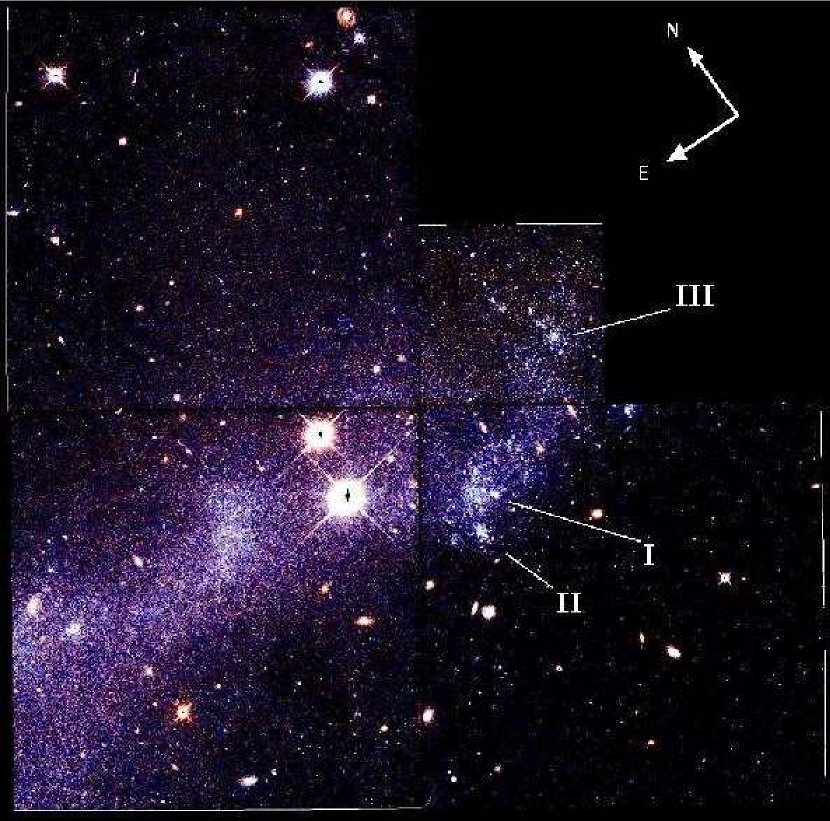
Figure 2.— True-color image of our HST field, where red has been assigned to the F814W image, blue to the F555W, and green to an image made from a combination of both filters. The extent and orientation of the field is outlined in Fig. 1. The three star formation regions studied by Mirabel et al. (1992) are marked along the bar-like structure that extends westward from the two bright stars.

A color image of the HST mosaic is shown in Fig. 2, and a visual inspection of the image gives a clear impression of the population, even without the formality of a color-magnitude diagram (CMD). The light of the tidal tail region imaged is dominated by bright blue stars indicative of a young stellar population (which contrast strongly with the reddish background galaxies). Fainter and redder stars indicative of an older population can also be seen. The youngest and brightest blue stars are located along a bar-like structure that extends from the two bright foreground stars in the upper right corner of the WF3, crosses the upper left corner of the WF4, and ends in the lower right corner of the PC. These stars form groups that look like OB associations, and the three most prominent ones coincide with the location of the three Hii regions studied by MDL92. Following that study, we refer to these regions as Regions I, II, III, and have labeled them as such in Fig. 2. Besides these active sites of star formation, another concentration of young stars can be seen in the WF3 chip, East of the two foreground stars.

The paper is organized as follows. The data reduction and calibration are presented in §2, and the resulting CMD is used in §3 to find the distance to the Antennae. We interpret the CMD with the aid of that of NGC 625 (a star forming dwarf irregular galaxy) and theoretical isochrones, and the distance modulus is then found using the luminosity of the tip of the red giant branch of the old population. The stellar content of the NGC 4038 tail is discussed in §4, and in particular, we discuss the spatial distribution of populations as a function of age in §4.1. A number of stellar associations are defined, and their morphology is compared to the central star clusters in §4.2. Their CMD is interpreted in §4.3, and an estimate of the mass in young and old stars is obtained in §4.4 (plus Appendix B) and §4.5, respectively. In order to interpret the luminosity function of the young population, a model of constant and continuous star formation is developed in Appendix B.3, and the luminosity function of the old population is compared to that of a Virgo dwarf elliptical in Appendix A. Our conclusions are given in §5.

2. Observations, reductions and calibrations

The field centered at $(\alpha,\delta,\rm epoch)=$ ($12$:$01$:$25.6$, $-19$:$00$:$31.9$, J2000) was imaged on November 23 and 24 1998, and January 4 and 5 1999. The outline of the HST wfpc2 field of view is indicated on a Digital Sky Survey (DSS) image of NGC 4038/9 in Fig. 1. Four filters were employed, for a total observing time of 1.4h in F336W, 0.7h in F450W, 2.1h in F555W and 2.9h in F814W. The exposure times for the two shortest wavelength filters were not long enough to allow the detection of stars, so our emphasis will be on the F555W and F814W frames.

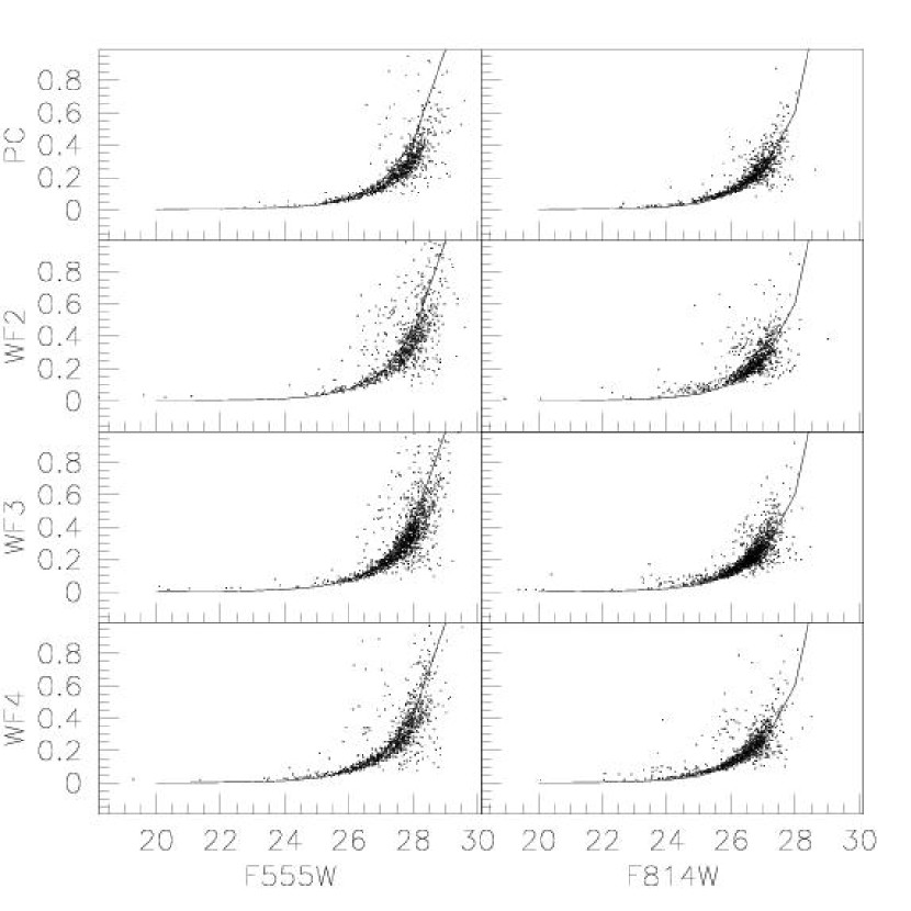
Figure 3.— allframe internal photometric errors. Absolute errors (in magnitudes) for the two filters are plotted in the left ($F555W$ filter) and right ($F814W$ filter) columns vs. the apparent magnitude. The solid curves represent the expected error based on the wfpc2 exposure time calculator.

2.1. Reductions

Our procedures for data reduction and calibration are based on the daophot II/allframe package (Stetson 1987, 1994). The procedures have been thoroughly described in Piotto et al. (2002) and Saviane et al. (2003), so only the general scheme is recalled here, which involves (a) image pre-processing, (b) profile-fitting photometry within a small radius, (c) correction for time-dependent charge-transfer efficiency (CTE), (d) growth-curve analysis and correction to total magnitudes, (e) calibration to the standard system, and finally (f) astrometry.

The images are prepared for the photometry by masking out vignetted pixels, and bad pixels and columns. The coordinates of detected sources are measured from a master frame, combining all of the images in all filters. These positions are used by allframe, which performs the photometry by fitting a point-spread-function (PSF) simultaneously to all stars of the individual frames. Since there are not sufficiently bright and isolated stars in any of the four chips, we are not able to construct the PSFs. Instead, we use the models extracted by P.B. Stetson (private communication) from a large set of uncrowded and unsaturated HST wfpc2 images. The resulting F555W and F814W magnitude lists are combined to create a raw color-magnitude (CMD) diagram.

2.2. Calibration

Table 1Photometry of Individual Stars.

ID	RA	DEC	$V_{0}$	$F555W_{0}$	$\epsilon_{F555W}$	$(V-I)_{0}$	$C_{0}^{\rm HST}$	$\epsilon_{C^{\rm HST}}$	#
1	12:01:28.625	-18:59:06.43	18.219	18.244	0.021	0.880	0.870	0.027	2
2	12:01:25.333	-19:01:34.86	19.277	19.302	0.023	1.102	1.089	0.027	4
3	12:01:25.106	-18:59:33.80	19.617	19.639	0.035	0.675	0.667	0.039	2
4	12:01:32.635	-19:00:32.12	20.102	20.126	0.035	0.717	0.709	0.037	3
5	12:01:25.439	-18:59:44.37	20.276	20.298	0.023	1.306	1.290	0.026	2
6	12:01:32.127	-19:00:56.46	20.372	20.298	0.015	2.875	2.830	0.141	3
7	12:01:28.752	-19:00:41.55	21.036	21.058	0.020	0.639	0.632	0.110	3
8	12:01:29.779	-19:00:08.29	21.092	21.117	0.029	1.017	1.004	0.034	2
9	12:01:27.784	-19:01:30.55	21.360	21.382	0.020	1.290	1.274	0.027	4
10	12:01:32.175	-19:00:46.49	22.170	22.151	0.023	2.248	2.215	0.027	3
11	12:01:30.112	-19:01:20.58	22.355	22.338	0.026	2.210	2.178	0.030	3
12	12:01:29.672	-19:00:53.06	22.617	22.530	0.026	3.000	2.953	0.030	3
13	12:01:25.546	-19:00:18.67	22.747	22.756	0.019	0.198	0.196	0.026	1
14	12:01:25.275	-19:00:39.61	23.209	23.230	0.048	0.569	0.563	0.063	1
15	12:01:25.086	-19:00:58.72	23.367	23.380	0.029	0.311	0.307	0.035	4
16	12:01:24.941	-19:00:41.77	23.392	23.416	0.021	0.797	0.788	0.028	1
17	12:01:27.231	-19:00:55.47	23.462	23.468	0.020	0.132	0.131	0.032	4
18	12:01:28.399	-19:01:23.96	23.505	23.529	0.029	0.832	0.823	0.035	4
19	12:01:25.583	-19:00:29.44	23.686	23.699	0.027	0.293	0.290	0.035	1

Note. — The coordinates are J2000, $C_{0}^{\rm HST}=(F555W-F814W)_{0}$, and # is the wfpc2 chip number, with 1 = PC, 2 = WF2, etc. The complete version of this table is in the electronic edition of the Journal. The printed edition contains only a sample.

In the next step, the photometry is calibrated to the standard system, following Dolphin (2000; D00), and assuming an average reddening in front of NGC 4038/9 of $E_{B-V}=0.046$ (Schlegel et al. 1998). This procedure accounts for both the time/counts dependence of the CTE and the variation of the effective pixel area across the wfpc2 field of view, and it yields final calibrated magnitudes in the Johnson–Kron–Cousins and the HST photometric systems.

The aperture corrections (to the reference aperture of $0\farcs 5$ of Holtzman et al. 1995; H95) could not be computed in the usual way, since we lacked the necessary bright isolated objects. Thus, we followed an approach closely resembling that of Ibata et al. (1999). Artificial images were created using the iraf/mknoise task, which reproduced the observed background+noise of our reference scientific frames (one frame per filter and per wfpc2 chip). On this background, the daophot/add routine was used to add a number of stars spanning an instrumental magnitude range from $14$ to $20$, making use of the available PSFs. For the details of this process, see Saviane et al. (2000). These artificial images were finally used to compute the aperture corrections, with uncertainties of $\pm 0.05$ magnitudes.

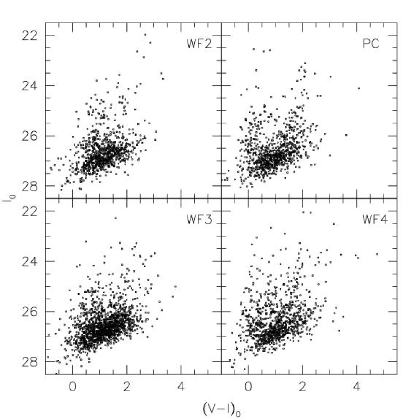
Figure 4.— The panels in this figure show the color magnitude diagram of each of the four wfpc2 chips, according to the labels in the upper-right corner. True $V-I$ colors and $I$ magnitudes are displayed along the abscissae and ordinates, respectively.

The J2000 positions of our objects were found through the metric task in the iraf/stsdas package. After processing, the world coordinates were appended to the photometry, and finally a single catalog was obtained by merging the four chip measurements. This catalog forms the basis of our discussion of the stellar content of this region of NGC 4038. We estimate a total systematic error of $\pm 0.05$ magnitudes, dominated by the uncertainty on the aperture corrections.

2.3. Characterization of the photometry

Figure 3 shows the resulting photometric errors as returned by allframe for both filters, and for each of the wfpc2 chips. One can immediately see that most of the stars are fainter than the $24^{\rm th}$ magnitude, and that below $F555W=28$, or $F814=27$, the incompleteness of the data starts to be severe. The typical trend of rising errors with magnitude can be seen (with smaller scatter in the PC and WF4 CCDs), and most of the stars in the field are affected by errors of a few $0.1$ magnitudes. The solid lines represent the expected photometric error based on the $S/N$ predicted by the wfpc2 exposure time calculator for the WF chips and an A0 star, within our daophot fitting radius of 2 px. The observed errors are (on average) $10\%$ smaller than expected for F555W, and ca. $20\%$ larger than expected for F814W. A few lines of the final photometric catalog are reported in Table 1, where the columns contain, from left to right, an identifier (ID), the J2000 equatorial coordinates (RA and DEC), the true Johnson and ST magnitudes ($V_{0}$ and $F555W_{0}$), the allframe photometric error on the ST mag ($\epsilon_{F555W}$), the true Johnson-Cousins and ST colors ($(V-I)_{0}$ and $C_{0}^{\rm HST}$), the photometric error on the ST color ($\epsilon_{C^{\rm HST}}$), and the wfpc2 chip number (#). The complete photometry is available in the electronic edition of the journal.

2.4. Comparison with groundbased photometry

The zero-point of our $V$ photometry was checked against the groundbased imaging of Hibbard et al. (2001). There are only five stars which are not saturated in the wfpc2 frames, and are bright enough to be measurable on the groundbased frames. Total magnitudes were then found within an aperture of $13\arcsec$, which was chosen after a growth curve analysis (the seeing was $1\farcs 8$ FWHM). The average difference is $<V_{\rm HST}-V_{\rm ground}>=0.09\pm 0.15$ for the five stars. Using only the three stars with more regular growth curves, we find $<V_{\rm HST}-V_{\rm ground}>=0.01\pm 0.11$. The two magnitude scales are then consistent within the mutual errors ($0.02$ magnitudes for the groundbased photometry, see Hibbard et al. 2001).

We cannot make a similar test in $I$-band, since no suitable groundbased photometry exists. However, since the D00 recipe for the calibration has no free parameters, we believe that the hst zero-point for the $I$ band is as reliable as that for the $V$ band. Note that the same methods have given a good calibration of wfpc2 $I$ photometry for each of $7$ globular clusters of the Large Magellanic Cloud (Saviane et al. 2003).

2.5. NGC 625

In order to constrain the distance to our field in the Antennae, we compare our CMD to that of a well understood nearby galaxy with a similar stellar population, for which deeper photometry and a well measured CMD are available (see §3). Toward this end, we retrieved wfpc2 imaging of the dwarf irregular galaxy NGC 625 from the hst archive (Proposal ID=GO8708; PI=Skillman), and $V,\leavevmode\nobreak\ I$ photometry was obtained following the methods described above, and adopting $E_{B-V}=0.016$ (Schlegel et al. 1998). The data consist of $4\times 1300$ s exposures in F555W and $8\times 1300$ s exposures in F814W, and thus reach limiting magnitudes comparable to those reached for NGC 4038/9.

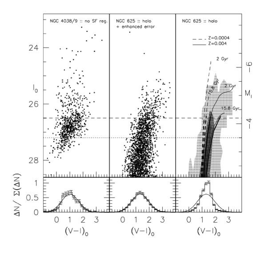
Figure 5.— The left and right panels show the CMDs of the NGC 4038 tail, and NGC 625, after selecting stars far from the star formation regions and adopting the distance moduli described in the text ($(m-M)_{0}=28.1$ mag for NGC 625 and 30.7 mag for NGC 4038/9). The central panel shows the CMD of NGC 625, after enhancing the photometric error. A set of isochrones from Girardi et al (2000) is overplotted to the NGC 625 diagram in the right panel , in order to illustrate the RGB (heavy lines) and AGB evolutionary phases. A greyscale plot has been adopted for this CMD ($3$ levels, from $1$ to $130$ in steps of $43$ counts), in order to better visualize the theoretical loci. In each panel, the dashed line marks the average luminosity of the RGB tip, $M_{I}=-4.2$. The bottom panels show, for each CMD, the histogram of the color distribution, for stars brighter than $M_{I}=-3.5$ (dotted line). A Gaussian of $\sigma_{V-I}=0.64$ is plotted over each histogram.

3. The distance to NGC 4038/9

In order to estimate the distance to NGC 4038/9, we need to understand the CMD of the NGC 4038 tail in terms of stellar evolutionary phases, and thus to assign absolute luminosities to its stellar populations. As we see in Fig. 3, the CMD is heavily affected by photometric errors, so its interpretation is not straightforward. For this reason, we decided to compare it to that of NGC 625. This is a star forming dwarf irregular galaxy in the Sculptor group, whose members have distance moduli in the range $26$-$28$ (e.g. Jerjen, Freeman & Binggeli 1998). Thus, it should have a stellar population comparable to our region, and we expect to see much better the various sequences, since its distance modulus is $\sim 4$ mag smaller, and the exposure times are almost the same.

3.1. Interpreting the CMD of the NGC 4038 tail

Figure 4 presents the color-magnitude diagrams constructed for each of the four wfpc2 chips. The bright blue and red stars seen in the CMDs belong to the tail’s youngest populations (see §4.1 below and Fig. 7). There is also a rise in star counts below $I_{0}\sim 26$, which could be due either to the red giant branch (RGB) tip, or to the upper envelope of the asymptotic giant branch (AGB), almost $1$ mag brighter. The RGB of the oldest populations is typically the most conspicuous bright-red feature of the CMD of a dwarf irregular galaxy (see e.g. Nikolaev & Weinberg 2000). The AGB shares the color location of the RGB, extending to brighter luminosities, but it is a shorter lived evolutionary phase and hence less populated. As is well known (e.g. Da Costa 1998), the luminosity of the RGB tip is almost independent of age and metallicity for ages greater than $2$ Gyr and for metallicities $0.0004\leq Z\leq 0.004$. This produces a characteristic discontinuity in the luminosity function which is used as a standard candle (see e.g. Da Costa 1998 and Carretta et al. 2000). In the quoted metallicity range, we can assume a tip luminosity $M_{I}^{\rm tip}=-4.2\pm 0.25$.

In order to understand whether the bright red stars of the NGC 4038 tail belong to the RGB or the AGB, we search for the best match between the luminosity function (LF) of the old population of our region, and that of the old population of NGC 625. However, we cannot work with the original CMDs, because (1) the RGB/AGB of the old population is polluted by the RGB of the young population, and (2) the photometric errors in our CMD are much larger than those in NGC 625 at comparable absolute luminosities. Thus, even if the underlying theoretical LFs were the same, the RGB tip discontinuity for the NGC 4038 tail would be less pronounced than that of NGC 625, and a good match could never be made (see Madore & Freedman 1995 for a thorough discussion of the shape of the RGB LF vs. photometric error and AGB contamination).

Figure 6.— Comparison of the LFs of NGC 4038 (filled diamonds and error bars) and NGC 625 (shaded histogram and error bars) for stars selected far from star forming regions. The solid and dashed curves represent the results of applying a Sobel filter to the luminosity function of NGC 4048 and NGC 625, respectively. The lower panel shows the cumulates of the NGC 4048 $M_{I}$ (solid line), and that of the NGC 625 $M_{I}$, in the range $-5\leq M_{I}\leq-4$. The result of the Kolmogorov-Smirnov test is also displayed.

In order to overcome the first difficulty, we attempt to isolate the CMD of the old population by selecting stars far from star formation regions. In the case of NGC 625, this means selecting the southern $35\arcsec$ of the WF2 chip. For the NGC 4038 tail, we selected stars in areas away from the star forming regions described in §1. The resulting isolated CMD for the NGC 4038 tail is given in the leftmost panel of Fig. 5.

To address the second difficulty, the errors of the NGC 625 photometry were increased to match those of the NGC 4038 tail photometry, and then the number of stars was reduced by a factor $r$ in order to match the number of stars in the brightest part of the NGC 4038 tail CMD. Thus we added random errors of $\sigma_{V}=0.35$ to the $V$ photometry and $\sigma_{I}=0.25$ to the $I$ photometry of NGC 625, to match the errors on the NGC 4038 photometry at $I_{0}\approx 26$. The resulting degraded CMD for NGC 625 is given in the middle panel of Fig. 5. The lower panels of this figure show histograms of the color distribution for stars brighter than $M_{I}=-3.5$ (dotted line), in order to show that the photometrically degraded NGC 625 data has a similar spread in color as the NGC 4038 tail data.

Next, the two CMDs were compared for a range in the difference of distance moduli, and for a range in $r$, until the best match was found. The match was decided on the basis of a Kolmogorov-Smirnov (KS) test on the two cumulated $M_{I}$ vectors, in the range $-5.0\leq M_{I}\leq-4.0$. For the comparison, the Whitmore et al. (1999; hereafter W99) distance modulus was adopted as a first guess for the distance of the Antennae. With this procedure, we derive a best fit of $r=2.4$ and a distance modulus difference of $2.6$ mag. More importantly, the best fit is achieved when the discontinuity in the NGC 4038 tail LF coincides with the RGB tip of the NGC 625 old population. From the absolute magnitude of the RGB tip we then find a distance modulus $(m-M)_{0}=30.7\pm 0.25$ for the Antennae, and in turn $(m-M)_{0}=28.1\pm 0.25$ for NGC 625. The error is dominated by the uncertainty on the RGB tip luminosity (which could be reduced if we knew the metallicity of the old populations of the two galaxies). Instead, if we changed the difference in the two distance moduli by only $\pm 0.08$ mag, the probability of the coincidence as measured by the KS test would drop already below $90\%$.

Figure 5 shows the isolated CMD of NGC 625 shifted so as to produce the best match to that of NGC 4038. The rightmost panel shows a greyscale representation of the original CMD of NGC 625 halo, plus some representative isochrones from Girardi et al. (2000).

The loci of the evolved RGB for two ages and two metallicities are drawn with heavy lines, while those for the AGB are drawn with thin lines. Furthermore, dashed and solid lines distinguish the two metallicities. The isochrones illustrate several evolutionary features mentioned above. Specifically, that the luminosity of the RGB tip is almost independent of age and metallicity for ages greater than $2$ Gyr and for metallicities $0.0004\leq Z\leq 0.004$; that the AGB shares the color location of the RGB, but has a brighter termination and extends more to the red for more metal rich populations; and most importantly that there is a sharp rise in star counts below $M_{I}\sim-4.2$, due to the more densely populated RGB.

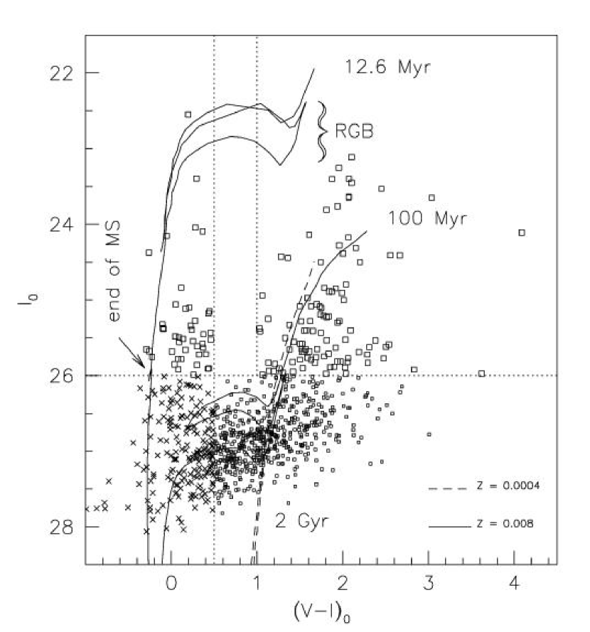
Figure 7.— The CMD of the PC field with three representative isochrones, assuming $(m-M)_{0}=30.7$. This diagram is used to define four subpopulations of stars: bright and faint blue MS stars younger and older than $\sim 12$ Myr (crosses and the large squares in the upper left region), bright red RGB and core helium burning stars younger than $\sim 100$ Myr (large squares in the upper right region), and faint red RGB and AGB stars older than $\sim 2$ Gyr (small squares). The dotted lines separate these four populations. Note that the vertical extent of the bright red region is larger than that of a single RGB (identified by the curly bracket), a sign of extended star formation.

The close match between the two CMDs is confirmed in Figure 6, where we display the two LFs, and the result obtained with the convolution with a Sobel edge detector (see Lee, Freedman & Madore 1993). We see the coincidence of both the main and secondary peaks of the two curves, where the higher maximum corresponds to the RGB tip, and the lower maximum corresponds to the upper envelope of the AGB. The lower panel of the figure confirms the coincidence in a quantitative way: the probability that the the two distributions in $M_{I}$ share a common parent is $91.8\leavevmode\nobreak\ \%$. Based on this experiment, we thus conclude that NGC 4038/9 is at a distance of $13.8\pm 1.7$ Mpc.

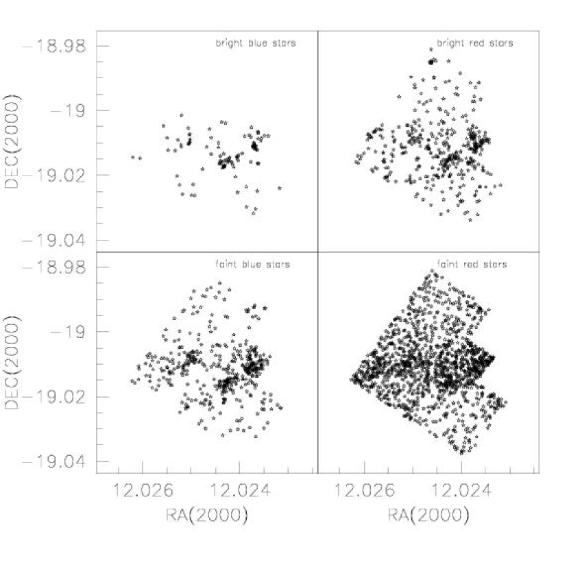
Figure 8.— J2000 positions of several subpopulations, identified by the labels in the upper right corner. These populations are those delineated in Fig. 7. The faint red stars, which we identify with old stars originally in the outer disk of NGC 4038, show a broader and uniform spatial distribution.

The Antennae is not the most distant system for which a distance based on the RGB tip has been attempted: Harris et al. (1998) used this method to find the distance of a dwarf elliptical galaxy of the Virgo cluster (at $\sim 16$ Mpc). In order to obtain the deepest possible LF, Harris et al. imaged the galaxy with the HST only in the $I$ filter. Thus, it is not possible to carry out a detailed comparison of the CMDs, as we did for NGC 625. On the other hand, the photometry of Harris et al. has photometric errors comparable to ours, permitting us to compare the two without any photometric manipulation. In appendix A we show that the close similarity of the two LFs adds further support to our distance modulus.

3.2. Comparison with previous distance determinations

All recent studies of the Antennae adopt a distance based on its redshift, but the results are not unique, even if the adopted heliocentric velocity is almost the same ($v_{\rm hel}\approx 1650$ km s^-1): variations of almost a factor of two are found in the literature (from e.g. $19$ Mpc, in Wilson et al. 2000, to $33$ Mpc in MDL92). In fact, different authors can adopt different values for the Hubble constant, and they can decide to correct for the solar motion in different ways (i.e. with respect to the Galactic center, to the Local Group, or no correction at all).

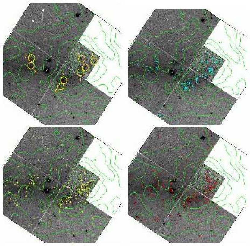
Figure 9.— Greyscale representation of the F555W frame with Hi column densities from the intermediate resolution datacube of Hibbard et al. (2001) and the location of various stellar populations (see Fig. 7) superimposed. The Hi density runs from $5\times 10^{19}\leavevmode\nobreak\ \rm cm^{-2}$ to $1.05\times 10^{21}\,\rm cm^{-2}$, in steps of $2\times 10^{20}\leavevmode\nobreak\ \rm cm^{-2}$. Top left panel: The location of the eight blue stellar associations identified in Table 2 and discussed in §4.2 are indicated by the numbered circles with a radius of $4^{\prime\prime}$. Top right panel: As in the first panel, but with the location of the bright blue stars indicated by cyan crosses. Bottom Left panel: As in the first panel, but with the location of the faint blue stars indicated by yellow crosses. Bottom Right panel: As in the first panel, but with the location of the bright red stars indicated by red crosses.

Therefore, a distance based on a standard candle is in dire need for this object, which is considered to be of great interest by a diverse community. In the past, this was attempted by Rubin, Ford & D’Odorico (1970), who were among the first to measure the radial velocity of the system ($v_{\rm hel}=1636$ km s^-1). They corrected the velocity to a Galactocentric value $v_{\rm rad}=1464$ km s^-1, and computed a distance of $19.5$ Mpc (for $H_{0}=75$ km s^-1 Mpc^-1). However, they disregarded it, since “for such a low value of the redshift, the effects of anisotropy in the velocity field make the determination of distance by means of the Hubble constant unreliable”. Instead, they used as their primary distance indicator the size of the disk Hii regions, which gave $D=6$ Mpc. Other distance indicators (the brightest stars and the 1921 supernova) gave distances ranging from $6$ Mpc to $13$ Mpc, due to the unknown amount of internal absorption. The authors also pointed out that NGC 4027 is likely physically linked to the pair, and the distance of the latter galaxy at the time was estimated $12.5\pm 2.5$ Mpc (de Vaucouleurs et al. 1968). In conclusion, although an accurate determination was not possible, there were indications of a distance shorter than that predicted by the redshift.

If, based on the Rubin et al. argument, we don’t put much confidence in the redshift distance, then our new distance determination is within the range of values discussed above. This means that the velocity of the galaxy is enhanced with respect to a pure Hubble flow, and we can see if this large peculiar velocity is compatible with modern flow models.

A recent, detailed model predicting the velocities of galaxies in the nearby Universe can be found in Tonry et al. (2000), who also provide the software to make one’s own calculations. The input of the model is the Supergalactic position of the object. If we assume our short distance, then the position of the Antennae is $(x,y,z)_{\rm SGB}=(-8.78,9.83,-4.09)\leavevmode\nobreak\ \rm Mpc$. At that position, the model predicts a radial velocity $v_{\rm rad}^{\rm mod}=1496\leavevmode\nobreak\ \rm km\leavevmode\nobreak\ s^{-1}$ in the cosmic microwave background (CMB) reference frame (and actually the total predicted velocity is almost aligned with the line of sight). The velocity of the Antennae in the same reference frame is obtained by adding the velocity of the Sun with respect to the CMB, which is $369\leavevmode\nobreak\ \rm km\leavevmode\nobreak\ s^{-1}$ in the direction $(SGL,SGB)=(116.72,-26.69)$ (Lineweaver et al. 1996). Its projection along the line of sight is $353.21\leavevmode\nobreak\ \rm km\leavevmode\nobreak\ s^{-1}$, so finally we obtain a velocity of the Antennae in the CMB reference frame of $v_{\rm rad}^{\rm obs}=1995.21\leavevmode\nobreak\ \rm km\leavevmode\nobreak\ s^{-1}$. The observed velocity is thus $500\leavevmode\nobreak\ \rm km\leavevmode\nobreak\ s^{-1}$ larger than the predicted one. The Tonry et al. model predicts a peculiar velocity dispersion of $187\leavevmode\nobreak\ \rm km\leavevmode\nobreak\ s^{-1}$ with respect to the local flow, so at our shorter distance the velocity of NGC 4038/9 is $2.7\leavevmode\nobreak\ \sigma$ larger than predicted by the model. While this is not an extreme discrepancy, one would still like to understand its origin. The discrepancy would be $+330\leavevmode\nobreak\ \rm km\leavevmode\nobreak\ s^{-1}$ at the W99 position, and $-660\leavevmode\nobreak\ \rm km\leavevmode\nobreak\ s^{-1}$ at the MDL92 position.

Figure 10.— Color-magnitude diagrams of $8$ associations of blue stars. The solid curves represent post-MS isochrones taken from Girardi et al. (2000), for ages of $4$, $12.6$, $39.8$, $126$, and $398$ Myr (corresponding to masses at the termination of the MS of about $42.6$, $15.8$, $8$, $4.5$, and $2.7\,M_{\odot}$), and a metallicity ca. $1/2$ solar ($Z=0.008$). Here we adopt $(m-M)_{0}=30.7$. The groups of stars have been selected from within a radius of $4\arcsec$ around sites of more active star formation. The plots are arranged in order of increasing RA, from left to right and top to bottom. Thus the top $4$ panels show CMDs from the PC chip star formation regions. They are followed by $2$ regions taken from the WF4 chip, and finally the bottom $2$ come from the WF3 chip. The stars bluer than $(V-I)_{0}=0.5$ (heavier crosses) have been used to construct the LFs, and among these, potential ionizing stars (i.e. $M_{I}\leq-5.23$) are plotted as filled triangles.

We can recall that the short distance found by Rubin et al. was in agreement with simple flow models of the time. In particular, using the kinematic model of the local supercluster of galaxies by de Vaucouleurs (1958), Rubin et al. predicted a distance $D=(1\pm 0.1)\times D_{\rm V}=10\pm 1$ Mpc, where $D_{\rm V}$ is the distance of the Virgo cluster. In the de Vaucouleurs (1958) model, the local supercluster had both a differential rotation and a recession velocity from its center, located in Virgo. The high velocity of the Antennae was then explained by its rotational velocity around the Virgo cluster center. Note that the distance to the Virgo cluster is now estimated $D_{\rm V}=16.4$ Mpc (Ferrarese et al. 2000), so the model would now give a distance to the Antennae of $D\simeq 15-18$ Mpc, and a revision of the model parameters might bring $D$ into agreement with our smaller value.

Another aspect of the problem is that flow models are valid in a statistical sense, and for relatively large portions of the Universe, so they can break down for individual objects. Indeed, the same discrepancy seen for the Antennae is present for one of the Tonry et al. galaxies near the position of the Antennae. Looking at their Fig. 11, one notes an object near $(x,y)_{\rm SGB}=-10,10\leavevmode\nobreak\ \rm Mpc$ whose radial velocity is, again, $\sim 300\leavevmode\nobreak\ \rm km\leavevmode\nobreak\ s^{-1}$ larger than that predicted by the model. Objects near the Antennae region start to feel the pull of the Great Attractor (GA), toward $SGL\sim 160$ deg, and Fig. 11 of Tonry et al. shows several other objects with residual velocities pointing toward the GA.

A final indication of a short distance is given by the distance to NGC 4027, if we still accept the physical association of the two objects. The value is still uncertain, but Pence & de Vaucouleurs (1985) adopt $10\pm 1.5$ Mpc from several distance indicators. Again, this value is smaller than that based on the recession velocity ($D\approx 14$ Mpc).

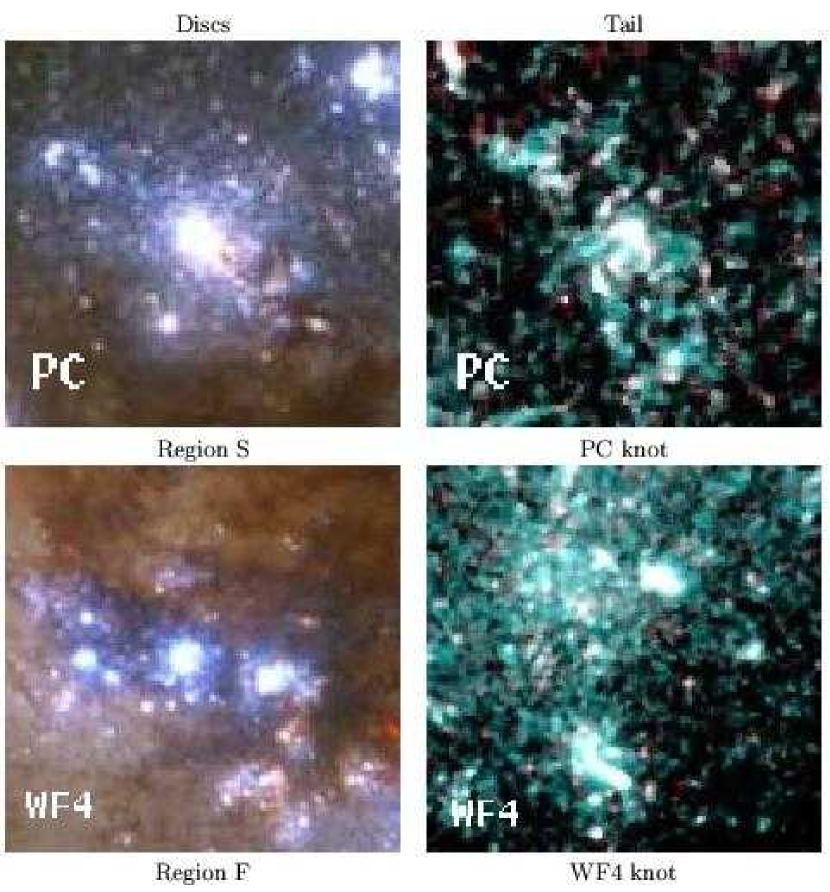
Figure 11.— Here we compare the visual appearance of two OB associations of the tidal tail to that of two ‘super’ clusters extracted from Whitmore et al. (1999). The size of the fields are $15\times 15$ and $10\times 10$ arcsec for the WF4 and PC images, respectively.

We note that the Tully “Nearby Galaxies Catalog” (Tully 1988) places NGC 4038/9 in group 22-1 at a distance of $21$ Mpc (based on distances to $5$ members of the group). The same value has been found for NGC 4033 in that group by Tonry et al. (2001). There are regions of the sky where structures with similar redshifts but different distances can overlap, but this is not the case for the Antennae, which are closer than the Great Attractor and away from the Virgo cluster (look at Fig. 20 of Tonry et al., at position $(x,y)_{\rm SGB}\approx(-10,10)$ Mpc). If our distance is confirmed, we must conclude that the association of the Antennae with group 22-1 is an optical superposition, as the Antennae are a factor $1.5$ closer.

4. The stellar content of the southern tidal tail

Insight into the star formation history of the tidal tail can be obtained from both the spatial distribution of stars selected from different regions of the CMD, and from direct analysis of the CMD. In the following sections we first analyze the spatial distribution of several subpopulations of stars, and then perform a more detailed comparison of the CMD of the young population to the theoretical isochrones. We then estimate the mass in young stars by several methods, using the main sequence luminosity functions of the star forming associations. Finally, we estimate the mass in old stars by comparing the luminosity function of stars located far from star forming regions to that of a dwarf spheroidal galaxy of the Local Group.

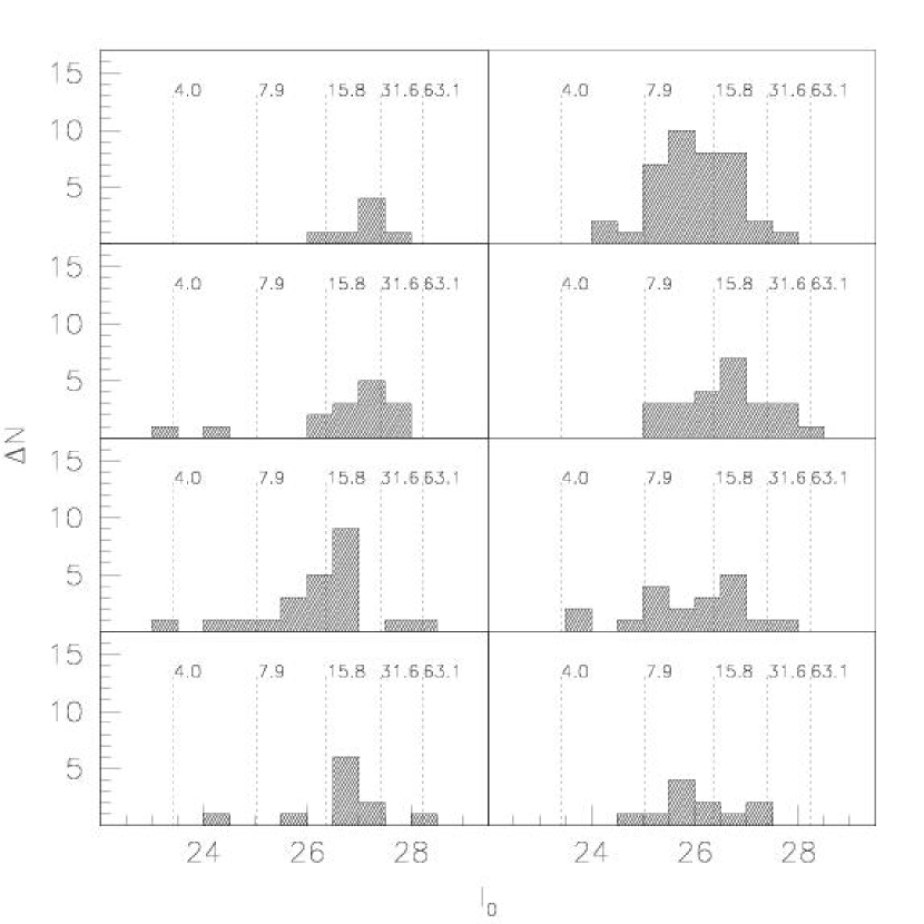
Figure 12.— The luminosity function of the blue stars identified in Fig. 10. The vertical dotted lines mark the end of the MS phase for several choices of the age, in Myr, and a metallicity $Z=0.008$. The arrangement of the panels is the same as that of the CMDs.

4.1. Spatial distribution of populations as a function of age

Fig. 7 shows the CMD from the PC chip, and three isochrones from Girardi et al. (2000) which have been placed at the distance of the Antennae for $(m-M)_{0}=30.7$. The $Z=0.0004$ isochrone (dashed line) represents the metal-poor, intermediate and old population. The two $Z=0.008$ isochrones show the CMD morphology of the younger populations. For these isochrones, we use the nebular oxygen abundance of $\approx 1/3$ solar measured by MDL92 which likely applies to all of the recently formed stars. Older stars likely have lower metallicities, so in the following we let $Z$ vary within a wide range (from $0.004$ to $0.02$).

Using Fig. 7, we define four regions of the CMD: bright blue, faint blue, bright red and faint red stars. The limit between bright and faint is set at $I_{0}=26$. Blue stars are stars bluer than $(V-I)_{0}=0.5$. Faint red stars are those redder than $(V-I)_{0}=0.5$, while bright red stars are those redder than $(V-I)_{0}=1$. These regions are delineated by dotted lines in Fig. 7. For the quoted distance modulus, and letting the metallicity $Z$ vary between $Z=0.0004$ and $Z=0.02$, we find that the regions delineating the bright and faint blue stars will contain mostly MS stars of ages less than or greater than $\approx 10$ to $\approx 13$ Myr, depending on $Z$. In Fig. 7 we see that the “hook” marking the end of the MS is right at $I_{0}=26$ for a $12.6$ Myr, $Z=0.008$ population. The region of bright red stars will contain mostly RGB and core helium burning stars younger than $\approx 80$ to $\approx 100$ Myr, again depending on $Z$. The limit $I_{0}=26$ is reached by the RGB tip of a $100$ Myr, $Z=0.008$ isochrone; the isochrone also shows that the progenitors of bright red stars were located inside the faint blue region. Finally, the faint red stars region will contain mostly RGB and AGB stars older than $\approx 2$ Gyr.

Table 2Photometric properties of the $8$ associations.

					blue				total
#	$RA$	$DEC$	$N_{\rm b}$	$N_{\rm T}$	$M_{I}$	$M_{V}$	$(V-I)_{0}$		$M_{I}$	$M_{V}$	$(V-I)_{0}$
1	12:01:24.53	-19:00:32.40	7	54	-6.4	-6.6	-0.1		-9.6	-8.3	1.2
2$\equiv$III	12:01:25.30	-19:00:40.32	39	96	-9.7	-9.5	0.1		-10.9	-10.1	0.8
3	12:01:25.63	-19:00:28.80	15	47	-8.8	-8.6	0.1		-10.2	-9.2	1.0
4	12:01:25.78	-19:00:45.37	24	60	-8.5	-8.5	0.1		-9.9	-9.0	0.9
5$\equiv$I	12:01:27.29	-19:00:54.72	23	64	-9.3	-9.1	0.2		-10.2	-9.5	0.7
6$\equiv$II	12:01:27.57	-19:01:01.56	19	41	-9.3	-9.2	0.1		-10.0	-9.4	0.6
7	12:01:30.13	-19:00:26.28	11	29	-8.0	-7.9	0.1		-9.0	-8.3	0.7
8	12:01:30.19	-19:00:35.28	11	32	-8.1	-7.8	0.2		-9.3	-8.3	1.0

Note. — The absolute magnitudes have been computed assuming the W99 distance modulus ($m-M_{0}=31.4$). Columns $RA$ and $DEC$ are the equatorial J2000 coordinates, $N_{\rm b}$ is the number of blue stars, and $N_{\rm T}$ is the total number of stars. Magnitudes and colors have been corrected only for foreground absorption and reddening. The associations number is given in the first column, and the labels I, II, and III identify the three star forming regions studied by MDL92.

The spatial distribution of each of these populations is shown in Figs. 8 and 9. Fig. 9 also shows the distribution of the starlight (greyscales) and the neutral atomic gas (contours; from the VLA data of Hibbard et al. 2001). With respect to the gas distribution, we see that the stars are well embedded within the ISM, with no signs of a relative displacement. Interestingly, a higher Hi density is observed in coincidence with the eastern bar-like structure, where the most active star formation is observed (see §4.2), and which contains the three Hii regions studied by MDL92. The youngest (bright blue) stars are clearly also concentrated along this structure. Moreover, the most active sites of star formation are located at the two extremes of the elongated structure, as is often observed in dwarf irregulars. Not surprisingly, both luminous and fainter main sequence stars follow a similar spatial distribution, with the youngest stars being the most tightly concentrated.

Bright red stars follow the distribution of main sequence stars, which indicates that the star formation started at least a hundred Myr ago. The faint red stars, which we identify with old stars originally in the outer disk of NGC 4038, show a broader and more uniform spatial distribution (Fig. 8), which gives an idea of the underlying structure of the tail. Notice also an apparent increase in surface density toward the North, probably connected with the low surface brightness extension of the tail first discussed by S78 (see also Fig. 1).

4.2. Young star forming associations

In order to characterize the recent star formation, we have selected those stellar associations which show an overdensity of stars within a few arcseconds, and which contain stars brighter than $I_{0}=27.5$ magnitudes (i.e. younger than $32$ Myr for $Z=0.008$ and our choice of distance modulus). Magnitudes and star counts were measured within a radius of $4\arcsec$, which corresponds to $\simeq 268$ pc for a distance modulus $(m-M)_{0}=$ 30.7, or $\simeq 370$ pc for the more commonly accepted distance modulus of $(m-M)_{0}=31.41$ (e.g. W99). The result is $8$ associations, whose locations are indicated in the top left panel of Fig. 9, and whose CMDs are shown in Fig. 10.

The CMDs of these $8$ associations are used to compute their integrated properties, which are summarized in Table 2. The table presents, from left to right, our identification number (and that of MDL92 when appropriate), the equatorial coordinates of the center of each region, the number of blue and total number of stars, then separately for the blue $(V-I)_{0}\leq 0.5$ and total populations: the absolute integrated $I$ and $V$ magnitudes and true color. Not surprisingly, the three associations with the highest flux in $V$ (i.e. those having $M_{V}\leq-9.4$) coincide with the three Hii regions studied by MDL92.

We now address the question of whether these regions contain enough ionizing stars to account for the H$\alpha$ fluxes observed by MDL92. To produce a significant ionizing flux, stars must be earlier than O5V, i.e. brighter than $M_{I}=-5.23$ (Cox 1999). We therefore select stars bluer than $(V-I)_{0}=0.5$ and brighter than $I_{0}=25.47$ in our CMD (drawn with black triangles in Fig. 10). We estimate the expected Lyman continuum luminosity ($L_{\rm Lyc}$) of these stars from Table 3 of Vacca et al. (1996). Given the Lyman continuum luminosities of each region, we calculate the expected H$\alpha$ luminosities using Table 2 of Rozas et al. (1999). The expected H$\alpha$ luminosities are $9\times 10^{38}$ erg sec^-1, $1.1\times 10^{39}$ erg sec^-1, and $6.8\times 10^{38}$ erg sec^-1 for regions I, II, and III, respectively. Comparing these to the H$\alpha$ luminosities measured by MDL92, converted to our smaller distance ($5\times 10^{38}$ erg sec^-1, $1.4\times 10^{38}$ erg sec^-1, and $2.8\times 10^{37}$ erg sec^-1 for regions I, II, and III respectively), we find that that there is more than enough ionizing radiation expected in these regions.

Another clue to the nature of the recent star formation is provided by a comparison of our modest sample of clusters with the so-called Super Star Clusters (SSCs) observed throughout central regions of the merging disks by Whitmore et al. (1999). Figure 11 shows such a side-by-side comparison, where the left column includes two examples of the W99 superclusters, and the right column includes two instances taken from our frames, where the three brightest knots are displayed (Regions I-III of MDL92). In order to compare the star formation regions at different resolutions, the top two images have been extracted from the PC chip ($0\farcs 05$ pixels), whereas the bottom two come from the WF4 chip ($0\farcs 10$ pixels).

Within the central regions, there are dozens of roughly spherical SSCs which contain more than $10^{5}$ M_⊙ of stars (W99). In contrast, the associations observed in the tidal tail are irregular in shape and contain less than a hundred stars brighter than $I_{0}=28$. Indeed, we see from Table 2 that even the brightest associations have $V$ luminosities falling in the faint bin of the W99 cluster LF, and most are close to their $M_{V}=-9$ faintest limit. It is then clear that within the tail we do not observe the kind of SSCs that have been produced in the “violent” central regions. The linear sizes look comparable to those of the central clusters, implying that the tail associations are in a much less dense environment. One might conclude that SSCs require the higher pressures found in the central regions in order to form (e.g., Jog & Das 1992, 1996; Elmegreen & Efremov 1997), while spontaneous star formation in the tail produces the kind of O-B star associations seen in dwarf irregular galaxies.

4.3. Comparison to theoretical isochrones

The CMDs for each of the associations are presented in Fig. 10, with post-MS isochrones taken from Girardi et al. (2000) drawn for ages between $4$ and $400$ Myr (for a distance modulus of $30.7$), and a metallicity $Z=0.008$. Figure 12 shows the luminosity functions for each association, with the luminosity of the termination of the MS (TMS) indicated by vertical dashed lines, for a range of ages and the same metallicity. Note that adopting the larger W99 distance modulus would shift all ages to younger values. For example, most stars of association $\#2$ would be older than $6$ Myr, instead of $8$ Myr.

The CMDs show a distinct blue MS up to $\sim 40$ Myr, but also a population of red supergiants, which are stars in either the RGB or the core helium burning phase. Since the bright red stars follow the spatial distribution of the blue stars (Figs. 8 and 9), we believe that the red populations belong to the same associations defined by the blue stars. If these associations represented single star formation episodes, then the RGB stars would be confined in an almost vertical CMD region with a relatively short extent in luminosity ($\sim 1$ mag) as shown in Fig. 7. Instead, the red vertical sequence extends for several magnitudes, as one can see in the most populated associations like $\#2$. Thus, it seems like stars have been forming for a few hundred Myr, possibly at a continuous rate.

The most populous association is $\#2$ (Region III from MDL92, also shown in the upper right panel of Fig. 11), with $39$ stars on the MS, and its CMD shows that most of its stars were formed more than $\sim 8$ Myr ago (see also the upper right panel of Fig. 12). Both the CMDs and LFs seem to indicate that there are few stars younger than $8$ Myr in any of the eight associations. However, it is interesting to note that the youngest stars are observed in associations $\#2$, $3$, $5$, and $6$, and that three of these coincide with the star formation regions studied by MDL92. In particular, the youngest stars are seen in association $5$, which coincides with association I of MDL92, who indeed found that this association is younger than the other two, containing stars whose age they estimated as $\leq 2$ Myr. We find stars as young as $3$ Myr in that association, and using an isochrone with slightly lower metallicity would reconcile our estimate with that of MDL92. For the other two associations, MDL92 estimated ages $\leq 6$ Myr, and indeed stars younger than that age are observed in associations $2$ and $6$.

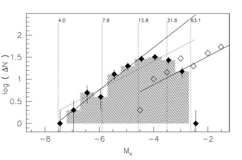
Figure 13.— Here we show the logarithmic integrated $M_{V}$ luminosity function of all the $8$ associations (filled diamonds and shaded histogram). The solid line is a power law with exponent $0.48$, as obtained by Cole et al. (1999) for IC 1613, fitted to the data for the brightest two magnitudes ($V_{0}\leq 26.5$ or $M_{V}\leq-4.2$). The open diamonds represent the main sequence LF of the LMC cluster NGC 2004 (Keller et al. 2000), to which a straight line has been fitted, yielding a slope $a=0.32\pm 0.04$. The dotted line represents a power law of the same exponent, fitted to the bright part of our LF. We assumed a LMC distance modulus and absorption of $(m-M)_{0}=18.5$ and $A_{V}=0.249$ respectively. The vertical dotted lines mark the end of the MS phase for several choices of the age, in Myr, and a metallicity $Z=0.008$. With these choices, we find the same age for NGC 2004 as that derived by Keller et al (2000), i.e. $15.8$ Myr.

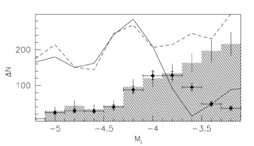
Figure 14.— The luminosity function of the Fornax dSph (shaded histogram with errorbars) is compared to that of the NGC 4038 tail (filled diamonds with errorbars). Notice the agreement at the bright end, prior to the point where the Antennae data suffer from incompleteness. The $x$ axis represents absolute $I$ magnitudes after correcting the two LFs for the respective distances and foreground absorptions of the two objects. The curves show the results of applying a Sobel filter to the NGC 4038 (solid curve) and Fornax LFs (dashed curve). Both curves show two main peaks, a higher one at $M_{I}=-4.2$ and a smaller one at $M_{I}\approx-5$. The first one corresponds to the RGB tip, while the second one is due to the upper AGB.

4.4. The mass in young stars

In order to characterize the star formation and to compare it to what is observed in dwarf galaxies, we estimate the stellar mass in the young and old populations. We start by computing the mass in young stars in the $8$ associations, based on their main sequence LF. Since all associations show extended star formation, we will treat star formation in the tail as a global process, and thus consider an integrated LF over all associations (see Fig. 13). The LF must be complete down to $M_{V}=-4.2$ (i.e. $V_{0}=26.5$), since our limiting magnitude is $V_{0}=28.5$ and completeness runs from $1$ to $0$ in $\approx 2$ mag for wfpc2 imaging in crowding conditions similar to ours (see e.g. Brocato, Di Carlo & Menna 2001, and Harris et al. 1998).

A realistic estimation of the mass in young stars needs a model of star formation, and a simple approach is developed in Appendix B.3. However, in order to guess the order of magnitude of the mass, and as a check of our model predictions, we start by computing this quantity under the hypothesis of a simple stellar population (SSP). After computing the mass in the $8$ associations, we extrapolate it to our whole region. The details of the process are left to Appendix B, while here we summarize the main results.

In order to estimate the mass of a SSP, we can either compare its LF to that of another SSP of known mass, or use the results of stellar population synthesis. Thus, we first compare the main sequence LF of the $8$ associations to that of a young populous cluster of the Large Magellanic Cloud (NGC 2004), and then we use the theoretical results of Renzini (1998) and Maraston (1998) to find the size of a young stellar population whose upper LF matches the observed LF.

In the first case, we find that the $8$ associations contain a factor $3.4\pm 1.2$ more stars than NGC 2004, or $(6.8\pm 2.4)\times 10^{4}\,M_{\odot}$ in young stars (using the cluster mass given by Mould et al. 2000). If we use the theoretical approach, then the resulting mass in young stars is $(2.1\pm 0.2)\times 10^{4}\,M_{\odot}$ (assuming a mass-to-light ratio $M/L_{\rm bol}=0.036$, and a Salpeter (1955) power-law mass function of exponent $\alpha=-2.35$). A few $10^{4}\leavevmode\nobreak\ M_{\odot}$ of young stars within the eight associations are then predicted under the SSP hypothesis.

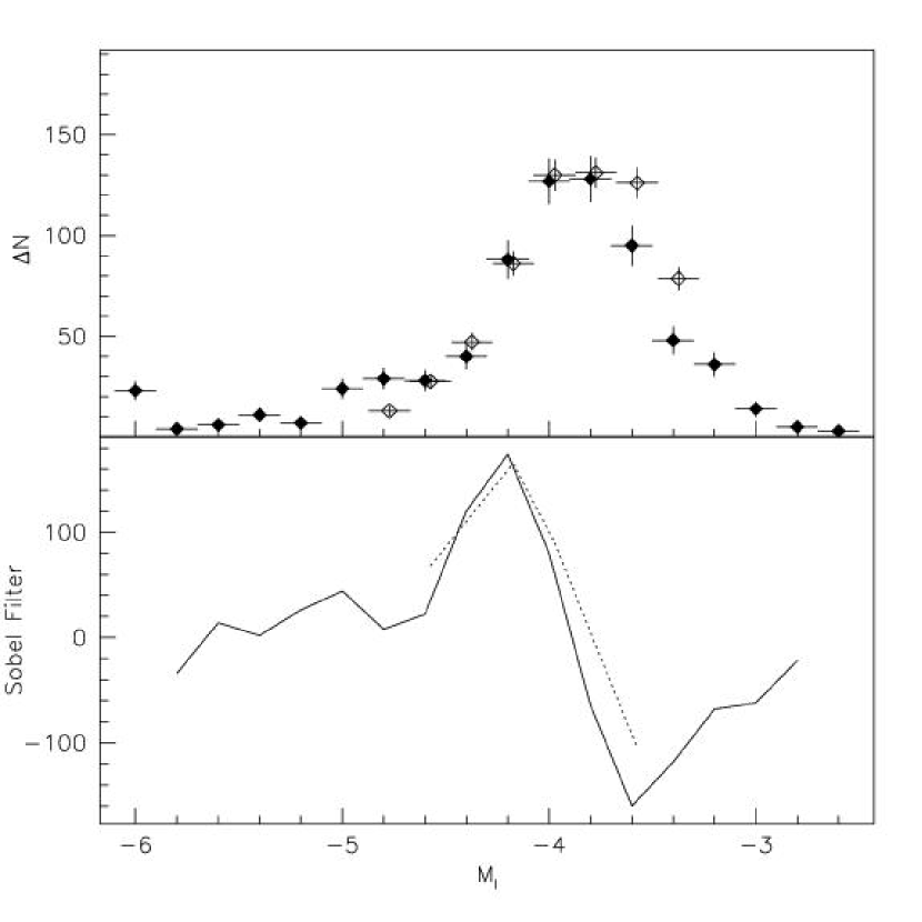
Figure 15.— This figure shows that the application of the Sobel filter to our Antennae data and to a published data set of comparable S/N give the same results. The $I$ band LF of the faint red stars in the NGC 4038 southern tidal tail (filled diamonds), and that of the Virgo cluster dwarf elliptical galaxy VCC1104 (open diamonds), are shown in the upper panel. The lower panel shows the LFs after convolution with the Sobel edge-detecting filter, where the NGC 4038 data are shown with a solid curve, and the VCC1104 data are shown as a dotted curve.

The inconsistency between the previous mass estimates could be another sign of an extended star formation history. Further, the brighter part of the LF is better fit by a power-law of exponent $\alpha=0.48$ ($0.1$ residual dispersion in $\log\Delta N$), than by our template SSP power-law of exponent $\alpha=0.32$ ($0.2$ residual dispersion), and according to Cole et al. (1999), an exponent $\alpha=0.48$ is a sign of continuous star formation. Therefore, in Appendix B.3 the mass of the young population is computed under this hypothesis. For this, we assume that star formation has been constant up to now, since a posteriori one can see that this simplification gives a reasonably good fit to the observed LF.

The model predicts the past SF rate as $\dot{M}=6\pm 3\times 10^{-3}\,M_{\odot}\,\rm yr^{-1}$, in agreement with the rate computed by MDL92 from the H$\alpha$ luminosity of the $3$ Hii regions (and scaled using our distance value). Such rate yields a mass of $1.1\times 10^{5}\,M_{\odot}$ produced during the last $20.6$ Myr spanned by our LF. This mass is larger than that computed above, so we see that the SSP hypothesis leads to an underestimate of the real mass.

By comparing the LF of all MS stars to that of the $8$ associations, we infer that in the entire region $(1.9\pm 0.2)\times 10^{5}\,\rm M_{\odot}$ were converted into stars since $20.6$ Myr ago. An absolute constraint on the mass of young stars comes from the total luminosity measured in this vicinity by MDL92 of $V=17.3$ mag, or $1.8\times 10^{6}L_{V,\odot}$, assuming a distance of $13.8$ Mpc. If we assume that 100% of this luminosity is due to young stars, it corresponds to $4.5\times 10^{5}M_{\odot}$ (for the $M/L$ of a Solar metallicity population of age $100$ Myr and Salpeter IMF), only a few times larger than our estimate. So the present star formation rate must have been sustained for only a few tens of Myr. The oldest stars seen in the associations must then have been produced during a period of lower star formation rate, or in discrete episodes.

4.5. The mass in old stars

As recalled above, stellar populations older than $\sim 2$ Gyr show a well populated RGB, which ends at an $M_{I}$ that is almost independent of age and metallicity (Fig. 5). Furthermore, the RGB luminosity function is a power law whose index is again almost independent of those two variables. As an example, Saviane et al. (1996) show that the LF of the dwarf spheroidal (dSph) in Tucana is similar to that of the Fornax dSph, yet Tucana hosts a globular cluster-like, metal-poor population while Fornax is a few Gyr old with an intermediate metallicity. Thus, we can estimate the mass of the old population of the tail by comparing the LF of its RGB with that of another old population of known mass. The old population was isolated from the young populations in §3.1, and its CMD was presented in Fig. 5, so we build the corresponding LF simply counting stars in magnitude bins. Unfortunately, the errors of the NGC 4038/9 photometry are so large that we cannot separate the AGB from the RGB based on their colors, so there will be some contamination of the LF by stars younger than $\sim 2$ Gyr. On the other hand, the contribution of the AGB to starcounts is $\sim 2$ orders of magnitude smaller than that of the RGB (see e.g. Fig. 6), so the mass that we compute will be close to the correct value.

With respect to an old population with known mass, we decided to use a dSph galaxy of the Local Group. These galaxies are ideal for this kind of comparison, since they are very close to the Milky Way, their physical characteristics are known with good accuracy, and they contain statistically significant numbers of old stars. In particular, we use the Fornax dwarf, since it was recently studied in Saviane et al. (2000), and its photometry is readily available. We take the RGB from their field C (the most populated one) and, before constructing the LF, we enhance the photometric errors as was done for our comparison with NGC 625 (§3.1). Moreover, we multiply the counts by a factor $4.8$, since the Fornax field contains less stars than the NGC 4038/9 field,

For a correct estimation of the mass, we must also remember that (a) field C of Saviane et al. contains only $5\%$ of the total population of Fornax (based on a King light profile and parameters from Irwin & Hatzidimitriou 1995); and that (b) the total area of the wfpc2 field is $4.1$ times larger than the portion where the old population was isolated.

The luminosity functions of the Fornax dwarf and of our NGC 4038/9 field are compared in Fig. 14, which shows their close agreement. For $-5\leq M_{I}\leq-4$, a KS test gives a $98.1\%$ probability that the two distributions share the same parent. The Sobel filter applied to the NGC 4038 LF gives the result shown by the solid line, and the dashed line shows the result for the Fornax LF. Like in the comparison with NGC 625, we see the coincidence of the primary peaks at $M_{I}=-4.2$, corresponding to the RGB tip, and even that of the secondary peaks at $M_{I}\approx-5$, corresponding to the upper AGB. The NGC 4038 curve starts to deviate from that of Fornax below $M_{I}=-4$, where incompleteness starts to affect our photometry.

The Fornax distance modulus and absorption were taken from Saviane et al. (2000; $(m-M)_{0}=20.7$, and $A_{I}=0.058$). Since that distance was based on the old value for the luminosity of the RGB tip, a $0.2$ mag correction was added to the distance modulus. In the comparison with NGC 625, its distance modulus was a free parameter, while now the Fornax distance is fixed. The very good match between the two LFs then means that Fig. 14 not only can be used to estimate the mass of the old population in the NGC 4038 tail, it also provides further strong support to our short distance.

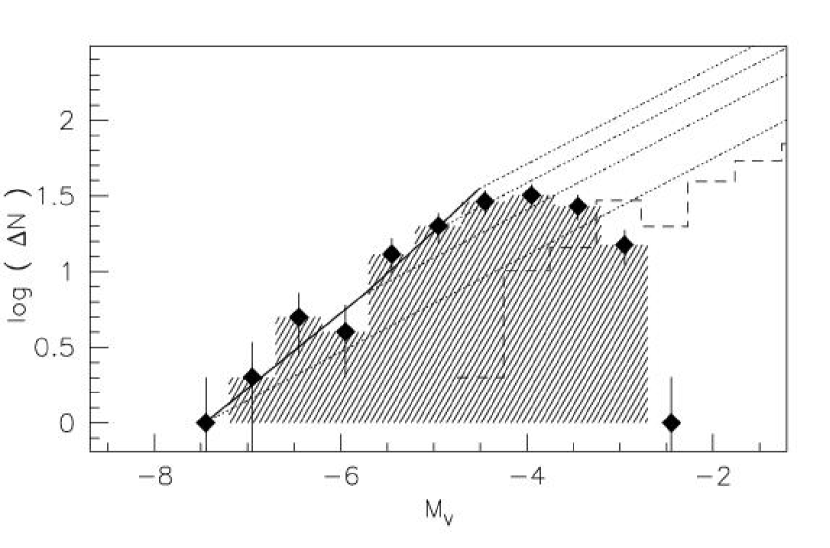
Figure 16.— The observed LF of the main sequence can be reproduced (heavy solid line) with the sum of $3.1$ LFs of simple stellar populations (dotted lines). We assume that the slope of the single LFs is equal to that of NGC 2004 (dashed histogram), and that the simple populations contain a factor $1.7$ more stars than the LMC cluster. The populations were generated at a constant rate during $18$ Myr, and all stars now evolved off the main sequence were removed from the LFs.

Based on the previous discussion, the number of old stars in the NGC 4038/9 field, $N_{\rm tail}$, is given by $N_{\rm tail}=N_{\rm Fornax}\times\ 4.8\times 4.1\times 0.05=0.98\times N_{\rm Fornax}$. This assumes a roughly constant density of old stars across the wfpc2 field. Since the mass of Fornax is $6.8\times 10^{7}\,M_{\odot}$ (Mateo 1998), assuming the same $M/L$ we find that there are $6.7\times 10^{7}\,M_{\odot}$ of old stars within the limits of our wfpc2 field.

Again, we can check whether this value is compatible with the total light measured by MDL92 in their field. If 100% of the $1.8\times 10^{6}\,L_{V,\odot}$ is in old stars, then it would correspond to $\approx 8\times 10^{6}\,M_{\odot}$, if the Fornax $M/L=4.4$ is used. The latter mass is smaller than our value, but our photometry reaches well below the surface brightness limit of ground-based imaging, so we conclude that our value of the mass for the old population is a reasonable estimate.

5. Summary and discussion

In this paper we have analyzed the stellar content of a region of linear dimension $\sim 8$ kpc, in the southern tail of the Antennae system of interacting galaxies. According to dynamical simulations (e.g. Barnes 1988), the material of the tail has been pulled out of NGC 4038 by the tidal field of NGC 4039 $\sim$ 450 Myr ago (for Milky Way sized progenitors), and previous groundbased studies of this area have shown that stars are now actively forming in a few regions (S78, MDL92). The wfpc2 camera on board of the HST has now been used to obtain, for the first time, broadband $F555W$ and $F814W$ photometry and astrometry of more than $4000$ stars within the region studied by MDL92.

A population of faint red stars is seen in the CMD. This population shows no clumping in its spatial distribution, and it was presumably ejected from the outer disks of the interacting galaxies. We have isolated a subsample of this population by selecting only stars from regions far from the active star forming areas. The selected sample shows a sharp cutoff in the LF at $I_{0}<26.5$. The LF is almost identical to that of the low surface brightness component of the star forming dwarf irregular galaxy NGC 625, and based on this comparison we interpreted the cutoff as the RGB tip of a few Gyr old population. This yields a distance to the Antennae of $13.8\pm 1.7$ Mpc, much shorter than the typically quoted $\sim 20$ Mpc. The choice of a shorter distance is reinforced by comparing the LF of this population to that of VCC1104, a dwarf elliptical galaxy in the Virgo cluster (see Appendix A), and to that of the Fornax dwarf spheroidal galaxy in the Local Group.

Our imaging with wfpc2 along with the VLA neutral hydrogen map of Hibbard et al. (2001) gives a better picture of the stellar populations at the end of the Southern tail of the Antennae. We find that the regions of most active star formation coincide with the Hi areas of highest density ($>8\times 10^{20}\leavevmode\nobreak\ \rm cm^{-2}$), and that the brightest young star forming associations are similar to those seen in dwarf irregular galaxies. In particular, there are two elongated structures that contain most of the associations, and one of them is the “bar” identified by MDL92. Our color-magnitude diagrams confirm the intuitive picture that the smooth structure of the tail is composed of older stars from the disks of NGC 4038/9 that were launched along with the gas, due to the interaction. The youngest stars are mostly concentrated in OB associations, but can also be found scattered over the whole region.

In contrast to the inner regions, there are no “super star clusters” seen in this region of the tail. The young tidal associations are more diffuse and have orders of magnitude fewer stars than the central star clusters. The eight most prominent associations have been used to study the recent star formation in the area. We are able to measure the luminosity function of their main sequence to reach stars as faint as $M_{V}=-4.2$ corresponding (roughly) to ages of $20$ Myr and masses of $14\,M_{\odot}$ (in the hypothesis of a short distance modulus). In this range, it would appear that the star formation has been continuous.

Considering the stellar mass budget of the whole area that we studied, by comparing the LF of the red-low surface brightness component to that of the Fornax dSph galaxy, we find that most of the mass ($\approx 6.7\times 10^{7}\leavevmode\nobreak\ M_{\odot}$) is contained in an old ($>2$ Gyr) stellar population, of order the stellar mass of Fornax itself. With a simple model of constant star formation we show there is a further $\approx 2\times 10^{5}M_{\odot}$ of stars formed in situ (including young stars outside the eight associations), within the last $20$ Myr.

Detailed investigations of the star formation process occurring well outside the boundaries of a disk or the potential well of a galaxy are rare. Mould et al. (1999) images the radio jet-induced star formation near NGC 5128, and finds a population similar to ours, with young OB associations but no massive star clusters. Clearly, star formation requires only the presence of gas of sufficient density, and not the large scale organizing gravitational potential of a disk, spiral arm, or galaxy.

One of the most important results of this work is the downward revision of the distance to the Antennae, which follows the first determination of the distance modulus based on a standard candle. This revision has consequences for the the nature of the TDG candidates, for the stellar populations within the inner regions, for the dynamical nature of the system, and for the dynamical models of the local Universe.

With respect to the TDG candidates, Hibbard et al. (2001) used the Hi kinematics to explore the dynamical nature of the regions studied by both MDL92 and S78. Specifically, they evaluate the ratio of the luminous mass, as inferred from the Hi and optical luminosity, and the dynamical mass inferred from the Hi line width and physical radius. They derive ratios of $M_{lum}/M_{dyn}\sim 0.3-0.7$ for a distance of 19.2 Mpc, where the range indicates stellar mass-to-light ratios ranging from $M_{*}/L_{B}=$ 0–5 (the analysis in §B.1 suggests a mass-to-light ratio near the bottom of this range). Since the baryonic mass scales as the square of the distance while the dynamical mass scales linearly with distance, a distance modulus of 30.7 requires revising these estimates downward by a factor of 1.4 (i.e. $M_{lum}/M_{dyn}\sim 0.2-0.5$). If either of these regions are self-gravitating entities, i.e. bona fide tidal dwarf galaxies, then most of their mass must be in the form of dark matter. This is quite hard to understand if they formed from disk material. Rather than witnessing the formation of a single large dwarf galaxy, we find it more likely that we are seeing several smaller scale regions forming stars. The mass scales of these regions are more typical of dwarf spheroidal galaxies than dwarf irregulars, and they may have more relevance to remnant streams around galaxies than the formation of dwarf irregular galaxies (Kroupa 1998).

With respect to the populations believed to result from the merger induced star formation taking place in the inner regions, all linear dimensions quoted in W99 would be reduced by a factor of $1.4$, so the effective radii of the youngest clusters created in the merger would now be comparable to those of Galactic globulars (W99 find a median effective radius $\sim 1.5$ times larger than that of GGCs). The young clusters’ LF would of course still be a power law, however, the bend found by W99 at $M_{V}\approx-10.4$ would now be a factor $2$ fainter in luminosity and the corresponding mass would be smaller, assuming the same $M/L$ value. W99 identified the bend with the characteristic mass of Milky Way globular clusters, although their value of $1\times 10^{5}\leavevmode\nobreak\ M_{\odot}$ is smaller than that of GGCs ($\approx 2\times 10^{5}\leavevmode\nobreak\ M_{\odot}$). With the shorter distance modulus, the mass of the bend would now be $\approx 5\times 10^{4}\leavevmode\nobreak\ M_{\odot}$, making this identification weaker.

With a smaller distance, the “Ultra Luminous” X-ray source population discovered by Fabbiano, Zezas & Murray (2001; see also Zezas et al. 2002, Zezas & Fabbiano 2002), while still extreme in its properties, becomes both less luminous (peak X-ray luminosity of $L_{X}=5\times 10^{39}$ ergs s^-1 vs. $2\times 10^{40}$ ergs s^-1) and less populous (6 instead of 18 with $L_{X}>10^{39}$ ergs s^-1). The X-ray sources in the Antennae are still luminous, but the new distance makes their luminosity function comparable to those found in other starburst galaxies (cf. Zezas & Fabbiano 2002).

Finally, with respect to the dynamical models of the local Universe, we compare the predicted and observed radial velocity of the Antennae at the new distance, using the Tonry et al. (2000) galaxy flow model of the local Universe, and find that the model predicts a velocity $500\leavevmode\nobreak\ \rm km\leavevmode\nobreak\ s^{-1}$ smaller than that of NGC 4038/9. The discrepancy would hold even if we used the W99 distance (it would then be $>300\leavevmode\nobreak\ \rm km\leavevmode\nobreak\ s^{-1}$).

Considering the importance of the distance estimate for a physical understanding of the Antennae, we would urge that the distance modulus be confirmed with deeper HST/ACS observations.

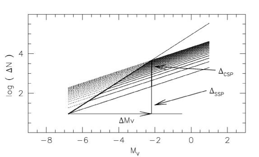
Figure 17.— Interpreting the LF of a composite stellar population (heavy solid line). We assume that it is made by the convolution of several LFs of simple stellar populations (thin inclined lines). The single populations are generated at a constant rate $\dot{n}$, and stars brighter than the termination of the main sequence are removed from the LFs (dotted lines). The figure has been obtained for $\dot{n}=0.21\,\,\,\rm Myr^{-1}$, from $100$ Myr to $4$ Myr ago. The labels identify parameters that are used in the text to develop our model.

Appendix A Comparison with a dwarf elliptical galaxy in the Virgo cluster

Harris et al. (1998) used the HST to image the Virgo cluster dwarf elliptical galaxy VCC1104 (=IC3388). Photometry in the $F814W$ filter was obtained with the wfpc2, it was calibrated with groundbased data, and then an LF was created with a bin size $\Delta I=0.05$. If we use the same bin size for the old population of the NGC 4038 tail, its LF turns out too noisy, since its CMD contains ca. half as many stars as that of VCC1104. The VCC1104 LF was then rebinned with $\Delta I=0.20$, and the counts were multiplied by $0.43$. The two LFs are compared in the upper panel of Fig. 15, where absolute magnitudes were computed assuming $(m-M)_{0}=30.7$ for the Antennae, and $(m-M)_{0}=30.98$ and $A_{I}=0.04$ for the Virgo dwarf (Harris et al. 1998). The lower panel shows the LFs after application of the Sobel filter, and both curves have a clear peak at $M_{I}=-4.2$, although with a large uncertainty. The figure shows that the two LFs are strikingly similar for $\sim 1$ magnitude down to $M_{I}\simeq-3.8$, where the incompleteness sets in. Hence, the two underlying populations must be similar as well, i.e. most of the faint red stars of the NGC 4038 tail must be RGB stars.

Appendix B Estimating the mass of young stars

B.1. Estimates of the mass under the SSP hypothesis

We start by comparing the brighter part of the LF with that of a young stellar cluster. Since the template LF must be statistically significant, we turn to the Large Magellanic Cloud (LMC) clusters. One of the youngest LMC clusters for which a LF is available is NGC 2004 ($16$ Myr, Keller et al. 2000), and its LF is plotted in Fig. 13 as open diamonds. The solid line through the points represents a fit to the LF, yielding a slope $\alpha=0.32\pm 0.04$. In the following discussion, this slope will be used as the template for a simple stellar population. Now since the two LFs have been formed using the same bins size, they can be compared directly. We fit a power-law of the same exponent to the bright part of our LF (as defined above), and the difference in zero point gives us the scale factor between the NGC 2004 LF and that of our region. The dotted line in the same figure represents the fit, which yields a scale factor of $3.4\pm 1.2$. The error has been estimated by allowing a $\pm 1\sigma$ variation in the logarithmic zero-point. Since the mass of the LMC cluster is $2\times 10^{4}\,M_{\odot}$ (Mould et al. 2000), this suggests that our eight associations contain a total of $(6.8\pm 2.4)\times 10^{4}\,M_{\odot}$ in young stars

The second way to estimate the mass of a SSP is the following theoretical one. The number of stars in a given mass range $m_{1}$ to $m_{2}$ on the MS, for a power-law IMF of exponent $\alpha$, can be expressed as in Renzini (1998):

$$N_{\rm MS}=\frac{A}{L_{\rm T}}\,L_{\rm T}\int^{m_{2}}_{m_{1}}m^{\alpha}dm$$

where $L_{\rm T}$ is the total luminosity of the population, $A$ is a normalization factor, and $A/L_{\rm T}$ depends on the age of the population. Assuming that our young stellar population can be approximated by a single $\simeq 30\,\rm Myr$ old burst (the youngest age available in the adopted models), then the computations of Maraston (1998) give $A/L_{\rm T}\simeq 0.007$ and a mass to light ratio $M/L_{\rm bol}=0.036$. Now we count $N_{\rm MS}=74\pm 9$ stars from $M_{V}=-7.7$ down to $M_{V}=-4.2$, and using the Girardi et al. (2000) isochrones (for $Z=0.008$), these luminosities can be translated into a mass range from $m_{1}=14\,M_{\odot}$ to $m_{2}=55\,M_{\odot}$. Introducing these numbers into the equation, for a Salpeter (1955) $\alpha=-2.35$ we obtain $L_{\rm T}=(5.9\pm 0.7)\times 10^{5}\,L_{\odot}$, or $M_{\rm T}=(2.1\pm 0.2)\times 10^{4}\,M_{\odot}$ using the quoted $M/L$.

B.2. Estimate of the mass under the extended star formation hypothesis

For this estimate, we use the model developed in the next section, which allows to compute the number of SSPs created per unit time ($\dot{n}_{\rm SSP}$) during the recent SF history, as a function of the slope of the composite LF $\alpha_{\rm CSP}$, the magnitude interval it spans $\Delta M_{V}$, and the corresponding time interval. In particular we have $\alpha_{\rm CSP}=0.49\pm 0.05$ (for $23.5\leq V_{0}\leq 26.5$), $\Delta M_{V}=3$ mag, and a time interval from $20.6$ to $2.5$ Myr ago. Inserting these values in Eq. (B2), we find a SSP formation rate of $\dot{n}=1.7\pm 0.8\times 10^{-7}$ SSPs yr^-1. Our model LF (heavy solid line) is plotted over the LF of the $8$ associations in Fig. 16. The model predicts that $3.1$ SSPs were created in $\approx 18$ Myr. Of course, we have already shown that stars older than $20.6$ Myr (and as old as, at least, $\sim 100$ Myr) are also present in the associations, but due to the incompleteness of our photometry, we cannot use the main sequence LF to probe the older star formation. In Fig. 16, the dotted line that reaches $M_{V}\approx-7.5$ represents the LF of one of the simple stellar populations. Comparing it to that of NGC 2004 (dashed histogram), we find that one generation produces $3.4\times 10^{4}\,M_{\odot}$, so in terms of mass, the past star formation rate was $\dot{M}=6\pm 3\times 10^{-3}\,M_{\odot}\,\rm yr^{-1}$, and we can finally estimate that $1.1\times 10^{5}\,M_{\odot}$ have been produced within the $8$ associations in the last $20.6$ Myr.

We can compare our SF rate to that inferred from the H$\alpha$ luminosity of the $3$ Hii regions measured by MDL92. The total luminosity is $\sum L(H\alpha)=3.9\times 10^{39}$ erg s^-1, for their distance of $33.2$ Mpc. Using the conversion of Hunter et al. (1986), and adopting our revised distance of $13.8\pm 1.7$ Mpc yields a star formation rate of $\dot{M}=9.5\pm 2.5\times 10^{-3}\,M_{\odot}\,\rm yr^{-1}$, which is in agreement, within the errors, with our derivation for the $8$ associations. Note also that a value $\eta=0.8$ in the Hunter et al. formula, would reconcile the star formation rate from the H$\alpha$ luminosity to our finding. The agreement between the two values is not unexpected, since most of the young stars are contained in the $3$ associations studied by MDL92.

B.3. A simple model of star formation

The purpose of our model is to explain the observed shape of the main sequence LF, in the case of continuous and constant star formation. The model is illustrated by Fig. 17, where we assume that such star formation can be approximated by the sum of a discrete number of simple stellar populations (SSPs). Each generation of stars produces a power-law LF which is added on top of that of the previous generation (thin solid inclined lines). As time passes, fainter and fainter stars die, so we truncate the single LFs at fainter and fainter magnitudes, with truncation magnitude as a function of time taken from the theoretical isochrones of Girardi et al. (2000). The observed LF (thick solid line) will then be the convolution of the LFs of several generations of stars, where the number of generations depends on the star formation efficiency and duration. The slope of the observed LF will be equal to that of a single generation of stars for magnitudes fainter than the current termination of the MS (TMS), while the slope will be larger for magnitudes brighter than the TMS. In this latter range, the slope will depend on the number of generations per unit time and on the slope of the single LF.

The previous reasoning can be formalized as follows. We assign variables $\alpha_{\rm SSP}$ and $b_{\rm SSP}$ as the slope and intercept of the single LF in the $M_{V},\Delta N$ plane shown in Fig. 17. Then, let’s express the star formation rate as the number of SSPs created in the unit time, $\dot{n}_{\rm SSP}$. In a given interval $\Delta t$, a number of populations $N_{\rm SSP}=\dot{n}_{\rm SSP}\times\Delta t$ is then created. In the absence of stellar deaths, the final LF would be a power-law of the same initial slope, and the zero point of this composite stellar population would be $b_{\rm CSP}=b_{\rm SSP}+\log(N_{\rm SSP})$. Instead, each LF we add will have a fainter TMS for increasing age, so each LF in the figure has been truncated at the corresponding $M^{\rm TMS}_{V}$ for its age. The age is $t=t_{\rm min}+i\times T_{1}$, for the $i^{\rm th}$ population, where $T_{1}=1/\dot{n}_{\rm SSP}$. Now from Fig. 17, we see that the slope of the brightest portion of the LF is $\alpha_{\rm CSP}=(\Delta_{\rm CSP}+\Delta_{\rm SSP})/\Delta M_{V}$, where $\Delta_{\rm CSP}$, $\Delta_{\rm SSP}$, and $\Delta M_{V}$ are defined in the figure. If we assume that the LFs of all generations have the same slope, then all quantities in the equation can be expressed as functions of that slope, the star formation rate, and the times of the beginning and end of the star formation. Thus, from the equation we can compute the star formation rate.

The horizontal offset is set by the difference between the magnitude of the TMS at the oldest and youngest ages. We found the time dependence of the TMS on the basis of the Girardi et al. (2000) isochrones. After plotting $M^{\rm TMS}_{V}$ vs. $\log t$ for several combinations of metallicity and age intervals, we found that a good approximation is

$$M^{\rm TMS}_{V}=3.29\times\log t-28.51$$ (B1)

which is valid in the interval $6.6\leq\log t\leq 9.5$, and for metallicities $0.004\leq Z\leq 0.02$. The $1$-$\sigma$ error on the coefficients is $1\%$, and the rms dispersion of the data around the fit is $0.4$ magnitudes. From expression (B1), it follows that $\Delta M_{V}=3.29\times\log(t_{\rm max}/t_{\rm min})$. As it has been shown above, the vertical offset introduced by creating $N_{\rm SSP}$ populations, is $\Delta_{\rm CSP}=b_{\rm CSP}-b_{\rm SSP}=\log N_{\rm SSP}$, and since $N_{\rm SSP}=\dot{n}_{\rm SSP}\times\Delta t$, it is $\Delta_{\rm CSP}=\log[\dot{n}_{\rm SSP}\times(t_{\rm max}-t_{\rm min})]$. Moreover, the vertical offset due to the simple stellar population LF is of course $\Delta_{\rm SSP}=\alpha_{\rm SSP}\times\Delta M_{V}=\alpha_{\rm SSP}\times 3.29\times\log(t_{\rm max}/t_{\rm min})$, where $\alpha_{\rm SSP}$ is the slope of the SSP LF. In conclusion, the expected slope of a composite population that has witnessed continuous star formation from $t_{\rm min}$ to $t_{\rm max}$, at a rate $\dot{n}_{\rm SSP}$, is

$$\alpha_{\rm CSP}=\alpha_{\rm SSP}+\frac{\Delta_{\rm CSP}}{\Delta M_{V}}=\alpha_{\rm SSP}+\frac{\log[\dot{n}_{\rm SSP}\,(t_{\rm max}-t_{\rm min})]}{3.29\,\log(t_{\rm max}/t_{\rm min})}$$

From this expression we can now obtain the number star formation rate as a function of the observables

$$\log\dot{n}_{\rm SSP}=(\alpha_{\rm CSP}-\alpha_{\rm SSP})\,\Delta M_{V}-\log\Delta t$$ (B2)

where an estimate of $\log\Delta t$ can be obtained from Eq. (B1) as a function of the observed range in $M_{V}$ along the LF.

References

- (1) Cox, A.N. (ed), 1999, Allen’s Astrophysical Quantities, Fourth Edition, Los Alamos, NM
- (2) Barnes, J.E., Hernquist, L. 1992, Nature, 360, 715 275
- (3) Brocato, E., Di Carlo, E., Menna, G. 2001, A&A, 374, 523
- (4) Carretta, E., Gratton, R. G., Clementini, G., & Fusi Pecci, F. 2000, ApJ, 533, 215
- (5) Cole, A.A., et al. 1999, AJ, 118, 1657
- (6) Da Costa, G. S. 1998, Stellar astrophysics for the local group: VIII Canary Islands Winter School of Astrophysics, 351
- (7) de Vaucouleurs, G. 1958, AJ, 63, 253
- (8) de Vaucouleurs, G., de Vaucouleurs, A., Freeman, K.B. 1968, MNRAS, 139, 425
- (9) Dolphin, A.E. 2000, PASP, 112, 1397 (D00)
- (10) Duc, P.-A., Mirabel, I.F. 1998, A&A, 333, 813
- (11) Duc, P.-A., Brinks, E., Wink, J.E., Mirabel, I.F. 1997, A&A, 326, 537
- (12) Elmegreen, B. G., & Efremov, Y. N. 1997, ApJ, 480, 235
- (13) Fabbiano, G., Zezas, A., & Murray, S.S. 2001 ApJ, 554, 1035
- (14) Ferrarese L., et al. 2000, ApJ, 529, 745
- (15) Girardi, L., Bressan, A., Bertelli, G., Chiosi, C. 2000, A&AS, 141, 371.
- (16) Gordon, S., Koribalski, B., & Jones, K. 2001, MNRAS, 326, 578
- (17) Harris, W.E., Durrell, P.R., Pierce, M.J., Secker, J. 1998, Nature, 395, 45
- (18) Hibbard, J. E., van der Hulst, J. M., Barnes, J. E., & Rich, R. M. 2001, AJ, 122, 2969
- (19) Holtzman, J.A., et al. 1995, PASP, 107, 1065 (H95)
- (20) Hunter, D.A., Gillett, F.C., Gallagher, J.S., Rice, W.L., Low, F.J. 1986, ApJ, 303, 171
- (21) Ibata, R.A. 1999, ApJS, 120, 265 (I99)
- (22) Irwin, M. & Hatzidimitriou, D., 1995, MNRAS, 277, 1354
- (23) Jerjen, H., Freeman, K. C., & Binggeli, B. 1998, AJ, 116, 2873
- (24) Jog, C. J., Das, M. 1992, ApJ, 400, 476
- (25) Jog, C. J., Das, M. 1996, ApJ, 473, 797
- Kauffmann & White (1993) Kauffmann, G. & White, S. D. M. 1993, MNRAS, 261, 921
- (27) Keller, S.C., Bessell, M.S., Da Costa, G.S. 2000, AJ, 119, 1748
- (28) Lee, M.G., Freedman, W.L., Madore, B. F. 1993, ApJ, 417, 553
- (29) Lineweaver, C. H., Tenorio, L., Smoot, G. F., Keegstra, P., Banday, A. J., & Lubin, P. 1996, ApJ, 470, 38
- (30) Madore, B.F., Freedman W.L. 1995, AJ, 109, 1645 (MF95)
- (31) Maraston, C., 1998, MNRAS, 300, 872
- (32) Mateo, M., 1998, ARA&A, 36, 435
- Mirabel et al. (1992) Mirabel, I.F., Dottori, H., Lutz, D. 1992, A&A, 256, L19 (MDL92)
- (34) Mould, J. R., et al., 2000, ApJ, 536, 266
- (35) Nikolaev, S., & Weinberg, M. D., 2000, ApJ, 542, 804
- (36) Pence, W.D., de Vaucouleurs, G. 1985, ApJ, 298, 560
- (37) Piotto, G., et al. 2002, A&A, 391, 945
- (38) Renzini, A., 1998, AJ, 115, 2459
- (39) Rozas, M., Zurita, A., Heller, C.H., & Beckman, J.E., 1999, A&AS, 135, 145
- (40) Rubin, V.C., Ford, W.K., D’Odorico S. 1970, ApJ, 160, 801
- (41) Salpeter, E. E. 1955, ApJ, 121, 161
- (42) Saviane, I., Held, E.V., Piotto, G. 1996, A&A, 315, 40
- (43) Saviane, I., Held, E.V., Bertelli, G. 2000, A&A, 355, 56
- (44) Saviane, I., Rosenberg, A., Piotto G., & Aparicio, A. 2003. In New Horizons in Globular Cluster Astronomy, ed. G. Piotto, G. Meylan, G. Djorgovski, and M. Riello, ASP Conf. Ser., 296, p. 402
- (45) Schlegel, D. J., Finkbeiner, D. P. & Davis, M., 1998, ApJ, 500, 525
- Schweizer (1978) Schweizer, F. 1978, in Structure and Properties of Nearby Galaxies, eds. E. M. Berkhuijsen and R. Wielebinski (Dordrecht,Reidel), p. 279 (S78)
- (47) Stetson, P.B. 1987, PASP, 99, 191
- (48) Stetson, P.B. 1994, PASP, 106, 250
- (49) Tonry, J.L., Blakeslee, J.P., Ajhar, E.A., & Dressler, A., 2000, ApJ, 530, 625
- (50) Tonry, J. L., Dressler, A., Blakeslee, J. P., Ajhar, E. A., Fletcher, A., Luppino, G. A., Metzger, M. R., & Moore, C. B. 2001, ApJ, 546, 681
- (51) Toomre, A., & Toomre, J. 1972, ApJ, 178, 623
- (52) Tully, B. 1988, Nearby Galaxies Catalog, Cambridge University Press
- (53) Vacca, W.D., Garmany, C.D., Shull, J.M., 1996, ApJ, 460, 914
- (54) Whitmore, B.C., Zhang, Q., Leitherer, C., Fall, S. M., Schweizer, F., Miller, B.W. 1999, AJ, 118, 1551
- (55) Wilson C.D., Scoville N., Madden S.C., Charmandaris V. 2000, ApJ, 542, 120
- (56) Zezas, A., Fabbiano, G., Rots, A.H., & Murray, S.S. 2002, ApJS, 142, 239
- (57) Zezas, A., & Fabbiano, G. 2002, ApJ, 577, 726
- Zwicky (1956) Zwicky, F. 1956, Ergebnisse der Exakten Naturwissenschaften, 29, 344