Ratio of energies radiated in the universe through accretive processes and nucleosynthesis

We present here a new determination of the ratio of energies radiated by active galactic nuclei and by stars and discuss the reasons for the apparently conflicting results found in previous studies. We conclude that the energy radiated by accretion processes onto super massive black holes is about 1 to 5% of the energy radiated by stars. We also estimate that the total mass accreted on average by a super massive black hole at the centre of a typical $10^{11}\,\textrm{M}_{\odot}{}$ galaxy is of about $7\,10^{7}\,\textrm{M}_{\odot}{}$.

1 Introduction

The universe is composed of various objects with a wide variety of emission processes. However, photons have three main origins: the big bang as the source of the cosmic microwave background (CMB), nuclear reactions in stars and gravity through accretion onto compact objects, especially super massive black holes (SMBH). Currently (at $z\simeq 0$), the ratio of the number of photons of CMB and stellar origin in the universe is of the order of 400. It is more difficult to estimate the ratio of the nuclear energy radiated by stars and the gravitational energy radiated by active galactic nuclei (AGN). Several recent studies have shown that the energy released by nucleosynthesis is evolving with cosmic time (Madau et al., 1996, 1998; Trentham et al., 1999; Somerville et al., 2001). It further seems that the star formation history roughly matches the evolution of energy release through accretion onto black holes (Dunlop, 1998; Franceschini et al., 1999), since both processes peak around $z\sim 2$. It is therefore possible to relate both phenomena and to estimate the energy ratio radiated by AGN and by stars over the history of the universe.

The determination of this ratio has been addressed several times in the literature. Dunlop (1998) constructed two models of the radio luminosity function of a sample of radio-loud quasars (RLQ), the first only considering luminosity evolution and the second combining luminosity and density evolution. He then related this luminosity to the mass accreted onto the central black hole and compared these curves with the star formation history. The two curves appear to be correlated, suggesting that when 1 $\textrm{M}_{\odot}{}$ is accreted by a SMBH in a radio loud quasar, $10^{7}\,\textrm{M}_{\odot}{}$ are used in the star formation process. Based on this relation, Courvoisier (2001) derived a ratio of the energy radiated by RLQ and stars of $E_{\textrm{\tiny RLQ}}$/$E_{\textrm{\tiny stars}}\sim 10^{-5}$ by assuming an accretion efficiency of 10 % for the RLQ and a stellar population made of 10 solar mass stars each radiating $4\,10^{52}$ ergs over their lifetime. Rather than considering only radio loud AGN, Franceschini et al. (1999) use the $0.5-2$ keV X-ray emission as a measure of the energy radiated by AGN. They find that when 1 $\textrm{M}_{\odot}{}\,\textrm{yr}^{-1}\,\textrm{Mpc}^{-3}$ is absorbed for star formation, the $0.5-2$ keV volume emissivity from AGN is $2.4\,10^{40}\ \textrm{ergs}\,\textrm{s}^{-1}\,\textrm{Mpc}^{-3}$. Considering that type I and II AGN bolometric luminosity is 250 times the $0.5-2$ keV luminosity and a stellar radiative efficiency of 0.001, Franceschini et al. (1999) finally obtain $L_{\textrm{\tiny bol}}\textrm{\scriptsize(AGN)}$/$L_{\textrm{\tiny bol}}\textrm{\scriptsize(SFR)}\sim 0.1$.

A different approach was followed by Fabian & Iwasawa (1999). Their estimate of this ratio is based on relations linking the bulge mass of a galaxy to both the mass of its central black hole and of its stars. They obtained a value of $\sim$ 0.2 for the ratio of the energy radiated by accretion processes and by stars, when assuming an accretion efficiency of 10 % for the AGN and the fact that one tenth of the stellar mass is used for nuclear fusion with an efficiency of 0.6 %.

Finally, Elvis et al. (2002) estimated that AGN contribute by at least 7 % to the total luminosity of the universe as derived from the diffuse background from submillimeter to ultraviolet wavelengths. They obtained this result by first deriving a lower limit of the AGN X-ray emission from the X-ray background (XRB) and by applying a bolometric correction determined with the average spectral energy distribution of quasars.

The aim of this study is to compare the various studies described above and to derive a new estimate of the ratio of gravitational energy released around SMBH to the energy released by nuclear fusion in stars. We first derive the radiation energy density due to stars in Sect. 2, then the corresponding value for accretion by SMBH based on the XRB in Sect. 3. The obtained ratio is compared with previous studies in Sect. 4, where we try to identify the origin of the discrepancies.

2 Energy radiated by stars

To estimate the energy radiated by stars in the universe we need to know both the energy release of a typical stellar population and the overall star formation history. Below, we start with the calculation of the stellar energy release, while the evolution of the star density will be described in Sect. 2.2.

2.1 Stellar energy release

We use the Starburst 99 models of Leitherer et al. (1999) to determine the typical stellar energy release. These models predict the spectrophotometric evolution of starburst galaxies between $10^{6}$ and $10^{9}$ years after the onset of star formation based on the stellar evolution models of the Geneva group (Schaller et al., 1992; Charbonnel et al., 1993; Schaerer et al., 1993a, b; Meynet et al., 1994). They consider the atmosphere models of Lejeune et al. (1997) and those of Schmutz et al. (1992) when the mass loss becomes important. A simple black body is used for cool stars with additional nebular continuum including free-free interactions below 912 Å and free-bound interactions above. These models have been computed with the isochrone synthesis method and are optimized for massive stars.

Since we are only interested in the total energy release of a typical population of stars during its whole life, we only consider the instantaneous star formation models of Leitherer et al. (1999) because in this case most of the energy is released before $10^{9}$ years. To assess the effect of changing the powerlaw index $\alpha$ of the initial mass function (IMF) of the stars we consider both a Salpeter IMF ($\alpha\!=\!2.35$) and a steeper Scalo IMF ($\alpha\!=\!3.3$). In both cases, the cutoff masses are chosen as $M_{\textrm{\tiny low}}\!=\!1\,\textrm{M}_{\odot}{}$ and $M_{\textrm{\tiny up}}\!=\!100\,\textrm{M}_{\odot}{}$. The effect of changing the metallicity $Z$ is taken into account by considering four different metallicities: $Z=0.040,0.020(=Z_{\odot}),0.008$ and $0.001$, but without chemical evolution in the models. As an example, we show in Fig. 1 the evolution of the bolometric luminosity of a $10^{6}\,\textrm{M}_{\odot}{}$ star cluster formed instantaneously with a solar metallicity ($Z=0.020$) according to the model of Leitherer et al. (1999). We extrapolate the bolometric luminosity from $10^{9}$ to $10^{10}$ years with a power-law in order to include the energy radiated during the final stages of stellar activity. This extrapolation is in good agreement with the earlier study of Charlot & Bruzual (1991).

Figure 1: Evolution of the bolometric luminosity of a $10^{6}\,\textrm{M}_{\odot}{}$ star cluster formed instantaneously with a metallicity $Z=0.020$ according to the model of Leitherer et al. (1999). The solid line is for a Salpeter IMF ($\alpha\!=\!2.35$) and the dashed line is for a Scalo IMF ($\alpha\!=\!3.3$). Only stars in the mass range between 1 and $100\,\textrm{M}_{\odot}{}$ are considered. Beyond $10^{9}$ years (dotted line), the model data have been linearly extrapolated up to $10^{10}$ years.

The total energy radiated by a $10^{6}\,\textrm{M}_{\odot}{}$ star cluster is obtained by integrating the bolometric luminosity over time.

Table 1: Energy radiated per unit of solar mass by stars $(E_{\textrm{\tiny rad}}/\textrm{M}_{\odot}{})_{\textrm{\tiny stars}}$ and the corresponding energy density $U_{\textrm{\tiny stars}}$ for different metallicities $Z$ and for a Salpeter ($\alpha\!=\!2.35$) or a Scalo ($\alpha\!=\!3.3$) IMF. The last column shows the corresponding energy density ratio radiated by AGN and by stars.

Z	$\alpha_{\textrm{\tiny IMF}}$	$(E_{\textrm{\tiny rad}}/\textrm{M}_{\odot}{})_{\textrm{\tiny stars}}$	$U_{\textrm{\tiny stars}}$	$U_{\textrm{\tiny AGN}}$/$U_{\textrm{\tiny stars}}$
		$10^{51}\ \textrm{ergs}\,\textrm{M}_{\odot}{}^{-1}$	$10^{60}\ \textrm{ergs}\,\textrm{Mpc}^{-3}$	$(10^{-2})$
$0.001$	2.35	4.16	1.29	2.8
	3.3	4.69	3.33	1.1
$0.008$	2.35	3.46	1.07	3.4
	3.3	3.39	2.40	1.5
$0.020$	2.35	3.09	0.96	3.8
	3.3	2.92	2.07	1.8
$0.040$	2.35	2.33	0.72	5.1
	3.3	1.71	1.21	3.0

The results are presented in Table 1 for the instantaneous stellar formation law, four different metallicities, and two different IMF. Since the bolometric luminosity is dominated by the energy radiated by the most massive stars, the flatter powerlaw index $\alpha$ of the Salpeter IMF provides a higher energy release than the Scalo IMF until $\sim 10^{8}$ years. Afterwards, the radiated energy being provided by less massive stars, a Scalo IMF gives more energy. Globally, the difference between the total energy radiated by a cluster of stars for a Scalo or a Salpeter IMF is quite small. On the other hand, the effect of increasing the metallicity is to decrease the stellar energy release. This effect can be understood as being due to an increase of stellar opacity with metallicity (Mowlavi et al., 1998). A quick comparison with Courvoisier (2001) shows that the values in Table 1 are consistent with his rough estimation that stars radiate $\sim 10^{51}\ \textrm{ergs}\,\textrm{M}_{\odot}^{-1}$ over their entire lives.

2.2 Evolution of the stellar density

Madau et al. (1996) first computed the star formation as a function of redshift. Since then, several authors have added new points to his diagram of the star formation rate (SFR) per unit of comoving volume as a function of the redshift. Different tracers have been used to derive the SFR, but now, it is common to use galaxy luminosities at different wavelengths. They can be converted into stellar formation rates using stellar population and galaxy spectral models, stellar formation scenarios and various IMF. Madau et al. (1998) propose conversion factors from luminosity to star formation rates ($L_{\textrm{\tiny UV}}=C\cdot SFR$) with different values of $C$ for a Salpeter IMF and a Scalo IMF. Somerville et al. (2001) compiled all the observations made in this way and present a homogeneous table of the comoving SFR density data for different cosmological models and a Salpeter IMF. Fig. 2 shows those data in the case of an Einstein-de Sitter cosmology and a Salpeter IMF.

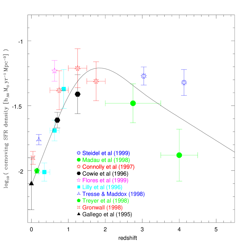
Figure 2: Evolution of the comoving SFR density for an Einstein-de Sitter cosmology and a Salpeter IMF from the data in Table A2 of Somerville et al. (2001). The solid line is a cubic spline matching as well as possible the observational constraints.

We calculate the stellar density $\rho_{\textrm{\tiny stars}}$ by integrating the star formation rate $\dot{\rho}_{\textrm{\tiny stars}}$ over the whole cosmic time:

$$\rho_{\textrm{\tiny stars}}=\int{\dot{\rho}_{\textrm{\tiny stars}}\,dt}\,.$$ (1)

If we consider a Friedman cosmological model, a flat universe, $q_{0}=0.5$, and $H_{0}=50\ \textrm{km}\,\textrm{s}^{-1}\,\textrm{Mpc}^{-1}$, Eq. (1) becomes:

$$\rho_{\textrm{\tiny stars}}=\int_{z_{\textrm{\tiny max}}}^{0}{\dot{\rho}_{\textrm{\tiny stars}}(z)\frac{dz}{H_{0}(1+z)^{2.5}}}\,.$$ (2)

With $z_{\textrm{\tiny max}}=5.5$ and $\dot{\rho}_{\textrm{\tiny stars}}(z)$ being the solid line adjusted to the data points of Fig. 2, we obtain:

$$\rho_{\textrm{\tiny stars}}=3.1\cdot 10^{8}\ \textrm{M}_{\odot}{}\,\textrm{Mpc}^{-3}\,.$$ (3)

This value is an average over the star formation history. Using the conversion factors given by Madau et al. (1998) and the table of Somerville et al. (2001), we deduce a different stellar density if we consider a Scalo IMF. Thus, for a Scalo IMF, an Einstein-de Sitter cosmology and $H_{0}=50\ \textrm{km}\,\textrm{s}^{-1}\,\textrm{Mpc}^{-1}$, we get:

$$\rho_{\textrm{\tiny stars}}=7.1\cdot 10^{8}\ \textrm{M}_{\odot}{}\,\textrm{Mpc}^{-3}$$ (4)

which is about twice the value for the Salpeter IMF. These results are only very weakly dependent on the cosmological model. Indeed, if we consider a $\Lambda$CDM cosmological model $(\Omega_{0}=0.3,\Omega_{\Lambda}=0.7)$ and calculate $\rho_{\textrm{\tiny stars}}$, we find a difference that is negligible ($\sim 0.2$ %) for both a Salpeter and a Scalo IMF compared to our previous values.

2.3 Energy density of the stellar radiation field

Having obtained the energy radiated by stars (see Table 1, column 2) and the star density for a Salpeter IMF (see Eq. 3) and for a Scalo IMF (see Eq. 4), we calculate the energy density due to stars as

$$U_{\textrm{\tiny stars}}=\rho_{\textrm{\tiny stars}}\cdot\left(\frac{E_{\textrm{\tiny rad}}}{\textrm{M}_{\odot}{}}\right)_{\textrm{\tiny stars}}\ \textrm{ergs}\,\textrm{Mpc}^{-3}\,.$$ (5)

The obtained values are reported in the fourth column of Table 1. Since $U_{\textrm{\tiny stars}}$ is proportional to $\rho_{\textrm{\tiny stars}}$ and $E_{\textrm{\tiny rad}}(\textrm{\scriptsize stars})$, we note that $U_{\textrm{\tiny stars}}$ decreases when $Z$ increases following the $E_{\textrm{\tiny rad}}(\textrm{\scriptsize stars})$ behavior and increases when the IMF slope is steeper.

3 Energy radiated by active galactic nuclei

To estimate the energy radiated by AGN, we use the observed X-ray background (XRB). This is motivated by the growing evidence that the XRB is emitted by discrete sources that are mainly AGN as proposed by Setti & Woltjer (1989). By adding the contribution of type I and II AGN, the observed XRB spectrum can indeed be well reproduced (Comastri et al., 1995; Gilli et al., 1999, 2001). Furthermore, it seems that the contribution of both massive X-ray binaries and supernovae to the XRB is negligible (Natarajan & Almaini, 2000). The emission from the hot interstellar medium is also small compared to the AGN contribution (Comastri et al., 1995). It is therefore possible to calculate the energy density in the AGN radiation field, $U_{\textrm{\tiny AGN}}$, from the observed XRB spectrum. Fabian & Iwasawa (1999) give the following analytic parametrisation that describes well the spectral energy distribution of the XRB as observed by HEAO-2 and ASCA for soft and hard X-rays:

$$I(E)=9\cdot E^{-0.4}\cdot\exp(-E/50\,\textrm{\tiny keV})\ \textrm{keV}\,\textrm{cm}^{-2}\,\textrm{s}^{-1}\,\textrm{sr}^{-1}\,\textrm{keV}^{-1}.$$ (6)

To relate this spectrum to the bolometric intensity of AGN, we use the mean ratio from the $2-10$ keV intensity to the bolometric intensity derived by Fabian & Iwasawa (1999):

$$L_{[2-10\,\textrm{\scriptsize keV}]}/L_{\textrm{\tiny bol}}\,\textrm{(RQQ)}=3.3\,\%.$$ (7)

This ratio is based on a compilation of spectral energy distributions of radio-quiet quasars (RQQ) by Elvis et al. (1994), which can be considered to be representative for the average emission of unobscured AGN. We further assume Fabian & Iwasawa (1999)’s hypothesis that the unobscured emission $E\,I(E)$ of AGN down to 2 keV can be considered as constant with a value of $38\,\textrm{keV}\textrm{cm}^{-2}\textrm{s}^{-1}\textrm{sr}^{-1}$ which is the XRB intensity at 30 keV. We then calculate the $2-10$ keV intensity of AGN as being $61\,\textrm{keV}\,\textrm{cm}^{-2}\,\textrm{s}^{-1}\,\textrm{sr}^{-1}$. From this last value and Eq. (7), we derive the bolometric intensity of AGN and we calculate the energy density of the AGN radiation field as

$$U_{\textrm{\tiny AGN}}=3.7\,10^{58}\ \textrm{ergs}\,\textrm{Mpc}^{-3}.$$ (8)

4 Discussion

We have independently determined the energy densities emitted both by stars and AGN in the universe. The obtained ratio $U_{\textrm{\tiny AGN}}$/$U_{\textrm{\tiny stars}}$ is given in the last column of Table 1 for two IMF and four different metallicities. We note that all values are between $10^{-2}$ and $5\,10^{-2}$. They slightly depend on the IMF slope and on the metallicity. Moreover, the choice of the cosmological model has a negligible effect as mentioned at the end of section 2.2. This ratio is expected to remain rather constant with cosmic time because the star formation history is similar to the AGN luminosity evolution towards higher redshifts (Dunlop, 1998; Franceschini et al., 1999).

4.1 Comparison between the different approaches

Our results differ by several orders of magnitude from other estimations of the energy ratio radiated by AGN and by stars. The different results extend from $10^{-5}$ (Courvoisier, 2001) to $10^{-1}$ (Fabian & Iwasawa, 1999; Franceschini et al., 1999; Elvis et al., 2002) through $4\,10^{-2}$ (this work). We cannot directly compare these values, because each study is based on a different approach to the problem; sometimes observational and sometimes approximative with the mass to energy conversion derived according to an efficiency $\varepsilon_{\textrm{\tiny rad}}$ through $E_{\textrm{\tiny rad}}=\varepsilon_{\textrm{\tiny rad}}Mc^{2}$.

Fabian & Iwasawa (1999) consider a typical galaxy and the contribution to the flux radiated both by the stars and the black hole hosted in this galaxy. They implicitly assume all galaxies with a black hole to host an AGN. However, the presence of a black hole does not mean that this galaxy is active. Some galaxies might have had an active phase, but are currently quiescent. Taking their ratio is equivalent to considering that every galaxy is currently active and contributes to the radiated energy of AGN. This leads to overestimate the energy radiated by AGN and thus to an overestimation of the AGN-to-star radiation ratio.

Franceschini et al. (1999) tackles the problem from the observational point of view starting with the energy radiated by the stars and the AGN to find a link between both phenomena. This approach is motivated by the apparent similarity between the cosmic evolution of the SFR and the AGN activity. In Courvoisier (2001), the sample of these active galaxies is based only on a radio survey. Therefore, this selection results in a sample of radio-loud galaxies which are only a small fraction of the whole AGN population. This leads to an underestimation of the accretion rate per unit of volume because there are many radio-quiet quasars that contribute to the energy radiated by accretion processes that are not taken into account. The use of the $0.5-2$ keV volume emissivity by Franceschini et al. (1999) allows one to include all AGN because they all radiate in the X-rays (Comastri et al., 1995; Gilli et al., 1999; Miyaji et al., 2000; Pompilio et al., 2000; Gilli et al., 2001) while only including a negligible contribution of other objects like star clusters or massive X-ray binaries (Gilli et al., 1999; Natarajan & Almaini, 2000; Gilli et al., 2001).

Elvis et al. (2002) also consider the AGN emission based on the XRB. However, they compare it to the total luminosity of the universe that is estimated from the diffuse background from submillimeter to UV wavelengths rather than only the stellar luminosity.

We conclude that the various studies mentioned above actually measure different quantities. Therefore, it is not possible to compare directly the values obtained by different groups.

4.2 Comparison between the different parameter values

In addition to the differences in the approaches and the measured quantities pointed out above, various studies use different values for the same parameters. The stellar efficiency $\varepsilon_{\textrm{\tiny rad}}$ used by Fabian & Iwasawa (1999) is 0.0006, but it is of 0.001 in Franceschini et al. (1999). Similarly, the ratio of the $2-10$ keV luminosity to the bolometric luminosity of the AGN is used in Fabian & Iwasawa (1999) and in this work, while Franceschini et al. (1999) consider instead the $0.5-2$ keV flux to derive a bolometric luminosity. Using the spectrum of Eq. (6), we can convert their bolometric correction to the one based on the 2-10 keV flux. Thus, we derive that their bolometric correction differs from the 3.3 % value of Fabian & Iwasawa (1999) by a factor of 3. It seems therefore that there is an accumulation of different factors explaining the diverging results in the literature. By taking the values of $\varepsilon_{\textrm{\tiny rad}}=0.0006$ and $L_{[2-10\,\textrm{\scriptsize keV}]}$/$L_{\textrm{\tiny bol}}=3.3\%$ from Fabian & Iwasawa (1999) and repeating the calculation of Franceschini et al. (1999), we obtain a value of $\sim 0.053$ for the ratio $L_{\textrm{\tiny bol}}\textrm{\scriptsize(AGN)}$/$L_{\textrm{\tiny bol}}\textrm{\scriptsize(SFR)}$, which tends to the value of 0.04 we obtain in this work for a solar metallicity and a Salpeter IMF.

In order to explicitly calculate $U_{\textrm{\tiny stars}}$ as defined here from the study of Elvis et al. (2002), we first subtract the quasar contribution to the total luminosity of the universe they give to get only the stellar background. We then obtain that $6.6\,10^{59}\ \textrm{ergs}\,\textrm{Mpc}^{-3}$ are radiated by stars which is quite similar to our result (see Table 1). Therefore, keeping their value of $U_{\textrm{\tiny AGN}}$, we estimate the ratio $U_{\textrm{\tiny AGN}}/U_{\textrm{\tiny stars}}\sim 0.067$ that becomes $\sim 0.046$ if we use the energy radiated by stars obtained in our study for a Salpeter IMF and a solar metallicity (see Table 1) instead of theirs. If we compare this to our results, we note that a difference also resides in the value of $U_{\textrm{\tiny AGN}}$. Considering Elvis et al. (2002)’s values of 48 $\textrm{keV}\,\textrm{cm}^{-2}\,\textrm{s}^{-1}\,\textrm{sr}^{-1}$ at 30 keV for the XRB instead of 38 $\textrm{keV}\,\textrm{cm}^{-2}\,\textrm{s}^{-1}\,\textrm{sr}^{-1}$ and their correction of a factor 1.6 to the bolometric correction, we recalculate our value of $U_{\textrm{\tiny AGN}}$ applying the same method as seen previously in Sect. 3. We find that the AGN emitted energy density of Elvis et al. (2002) is 1.5 times higher than ours. With this new derivation of $U_{\textrm{\tiny AGN}}$, we calculate a ratio $U_{\textrm{\tiny AGN}}/U_{\textrm{\tiny stars}}\sim 0.031$ for a Salpeter IMF and a solar metallicity that is a factor 2 lower than their value of 0.067. The difference comes from a lower $U_{\textrm{\tiny AGN}}$ and a higher $U_{\textrm{\tiny stars}}$, both effects combining to give a ratio twice lower.

Finally, it is worth noting that recent observations by Sarzi et al. (2001) lead to a smaller ratio of the central black hole mass to the host bulge mass than the value used by Fabian & Iwasawa (1999). By using their new result of $M_{\textrm{\tiny BH}}$/$M_{\textrm{\tiny bulge}}\simeq 0.002$ the ratio $E_{\textrm{\tiny AGN}}$/$E_{\textrm{\tiny stars}}$ found by Fabian & Iwasawa (1999) would have been of $\sim\!0.07$ instead of $\sim\!0.2$.

4.3 Relation between RLQ radio luminosity and AGN bolometric luminosity

Franceschini et al. (1999) and Courvoisier (2001) compared the star formation rate to the accretion history based on the observation either in the X-ray band or in the radio band. Every AGN is responsible for the X-ray emission but only a subset of AGN has a significant radio emission. Therefore, we easily get a link between these two classes of objects. When $1\ \textrm{M}_{\odot}{}\,\textrm{yr}^{-1}\,\textrm{Mpc}^{-3}$ is used by the star formation, $2.4\,10^{40}\ \textrm{ergs}\,\textrm{s}^{-1}\,\textrm{Mpc}^{-3}$ are emitted by the AGN in the $0.5-2$ keV band and $10^{-7}\ \textrm{M}_{\odot}{}\,\textrm{yr}^{-1}\,\textrm{Mpc}^{-3}$ is accreted onto the central black hole of a RLQ. If we transform the $0.5-2$ keV luminosity into the bolometric luminosity using $L_{[0.5-2\,\textrm{\scriptsize keV}]}$/$L_{\textrm{\tiny bol}}(\textrm{AGN})\sim 1.25$ % derived from Eqs (6) and (7) and if we consider an accretion efficiency onto the black hole of 10 %, we obtain that $3.4\,10^{-4}\ \textrm{M}_{\odot}{}\,\textrm{yr}^{-1}\,\textrm{Mpc}^{-3}$ is accreted by the AGN for a SFR of $1\ \textrm{M}_{\odot}{}\,\textrm{yr}^{-1}\,\textrm{Mpc}^{-3}$. Therefore, we can compare the luminosity of both the RLQ and the AGN as we get $\sim 10^{4}$ of difference between them. When $1\ \textrm{erg}\,\textrm{s}^{-1}\,\textrm{Mpc}^{-3}$ is radiated by the RLQ at 2.7 GHz, the complete population of AGN radiates about 3400 times more.

Furthermore, we can reconsider the method used by Courvoisier (2001) to determine $U_{\textrm{\tiny AGN}}/U_{\textrm{\tiny stars}}$. We have seen that we cannot directly compare his result to the others since they are not considering the same family of objects. Instead of using the analysis of RLQ by Dunlop (1998), we recalculate the ratio of Courvoisier (2001) using the analysis of the XRB of Franceschini et al. (1999). Therefore, we obtain a value of $E_{\textrm{\tiny AGN}}$/$E_{\textrm{\tiny stars}}\sim 0.015$ between the energies radiated by AGN and stars instead of RLQ and stars. This value becomes $\sim 0.020$ if we use our result of the energy radiated by stars for a Salpeter IMF and a solar metallicity (see Table 1). The initial inconsistency of a factor of a thousand has been reduced to only a factor of 2 between this last estimate and the one in Table 1.

4.4 Mass accreted by supermassive black holes

Based on our previous results we can estimate the total mass accreted by SMBH. If we consider a galaxy with a mass of $10^{11}\ \textrm{M}_{\odot}{}$ in stars, we can estimate the energy radiated by those stars from the value in Table 1 for a Salpeter IMF and a solar metallicity. Using the corresponding ratio of the AGN-to-stars energy release, we can then derive the energy radiated by the SMBH. By further assuming an accretion efficiency of 10%, we obtain that the total mass accreted by the SMBH is $6.5\,10^{7}\ \textrm{M}_{\odot}{}$. In general, the typical mass accreted by a SMBH in a galaxy can be calculated according to

$$\begin{split}M_{\textrm{\tiny AGN}}^{\textrm{\tiny accr}}(\textrm{M}_{\odot}{})&=2.2\cdot 10^{7}\,\left(\frac{0.1}{\varepsilon}\right)\!\left(\frac{\scriptstyle E_{\textrm{\tiny AGN}}/E_{\textrm{\tiny stars}}}{0.04}\right)\!\\ &\times\left(\frac{M_{\textrm{\tiny Gal}}}{10^{11}\textrm{M}_{\odot}{}}\right)\!\left(\frac{(E_{\textrm{\tiny rad}}/\textrm{M}_{\odot}{})_{\textrm{\tiny stars}}}{10^{51}\ \textrm{ergs}\,\textrm{M}_{\odot}{}^{-1}}\right)\,.\end{split}$$ (9)

We can also estimate this mass starting from the link given in the previous subsection. We have seen that when 1 $\textrm{M}_{\odot}{}$ of material is converted into stars, $3.4\,10^{-4}\ \textrm{M}_{\odot}{}$ is accreted onto SMBH. If we consider again a galaxy with a mass of $10^{11}\ \textrm{M}_{\odot}{}$ in stars, we estimate that $3.4\,10^{7}\ \textrm{M}_{\odot}{}$ is accreted onto the SMBH that is half of our previous estimate. This difference by a factor of 2 is the same as for the ratio $E_{\textrm{\tiny AGN}}$/$E_{\textrm{\tiny stars}}$ mentioned in Sect. 4.3.

5 Conclusion

We derived the relative contribution of AGN and stars to the radiation energy density of the universe. The results are given for different IMF and metallicities of the stellar population. The obtained values for the energy ratio released by AGN and stars are all between 0.01 and 0.05. In the case of a Salpeter IMF and solar metallicity we obtain a ratio of 0.04. This result cannot be compared directly with previous studies because the approaches as well as the values of some parameters used in the calculation differ from one study to the other. Actually, when using similar parameters and appropriate correction factors it seems that all previous studies do converge to values between 0.02 and 0.07 for the ratio of energy radiated by AGN and stars.

Since the CMB energy density is about $\sim 0.2\ \textrm{eV}\,\textrm{cm}^{-3}$, the energy density due to stars is of the order of $10^{60}\ \textrm{ergs}\,\textrm{Mpc}^{-3}\sim 0.02\ \textrm{eV}\,\textrm{cm}^{-3}$ and the AGN related radiation energy density is of about $8\,10^{-4}\ \textrm{eV}\,\textrm{cm}^{-3}$, the general picture resulting from this work is that the CMB contributes 10 times more than stars and 250 times more than AGN to the local energy density of background photons.

We also estimate that RLQ contribute about 3400 times less than the whole AGN family to the total accretion power in the universe and that the cumulated mass accreted on average by a SMBH is of about $6.5\,10^{7}\,\textrm{M}_{\odot}{}$.