Temporal Bias in the Clustering of Massive Cosmological Objects

Abstract

It is a well-established fact that massive cosmological objects exhibit a “geometrical bias” that boosts their spatial correlations with respect to the underlying mass distribution. Although this geometrical bias is a simple function of mass, this is only half of the story. We show using numerical simulations that objects that are in the midst of accreting material also exhibit a “temporal bias,” which further boosts their clustering far above geometrical bias levels. These results may help to resolve a discrepancy between spectroscopic and clustering mass estimates of Lyman Break Galaxies, a population of high-redshift galaxies that are caught in the act of forming large numbers of new stars.

I Introduction

Large-scale structure in the Universe is believed to have originated from a primordial Gaussian random field of matter fluctuations, the product of quantum fluctuations that were shifted to larger spatial scales during cosmological inflation [e.g.  1]. Cosmic Microwave Background observations show that when the Universe was 100,000 years old, the gaseous component was extremely smooth, with temperature variations $\sim 10^{-5}$. These tiny inhomogeneities, in concert with inhomogeneities in the unseen massive dark-matter, were amplified through gravitational instability, eventually forming the galaxies, clusters, and other cosmological objects we see today.

While the precise details of structure formation are highly complex, the simplicity of the initial random field allows us to easily compute the overall distributions of cosmological objects. Galaxies and galaxy clusters represent the peaks in the initial density distribution which accrete matter at the expense of the diffuse regions between them, and thus their number densities can be simply related to the number densities of the peaks of the initial random field. This technique has been applied most cleanly to galaxy clusters, whose densities and evolution provide strong constraints on the overall matter density ek96 .

Similarly, because the peaks in a random field are more clustered than the overall distribution, the spatial clustering of cosmological objects is stronger than the underlying mass distribution. Furthermore, this “geometrical bias” is a systematic function of the mass of these structures, an effect that has been well-studied analytically and numerically [e.g.  3, 4, 5].

Yet, this is only half of the story. Here we conduct a detailed numerical simulation that shows that the spatial correlation function of objects that are in the midst of accreting substantial amounts of material is significantly enhanced over that of the general population. This temporal bias causes them to mimic the properties of higher-mass structures, with important astrophysical implications as discussed below.

The structure of this work is as follows: In §2 we describe our numerical simulation, discuss our group-finding algorithms, and develop a robust definition of accreting groups. In §3 we present our results for the spatial correlation functions of these samples, and in §4 we discuss the astrophysical implications of our results. Further details of this study are given in sc03 .

II Simulations and Group Finding

Our numerical simulation traced the growth of primordial density fluctuations by dynamically evolving a large number of point test particles. The distribution of these particles was then used to determine the nonlinear evolution of the spatial correlation function of massive objects at late times. Driven by measurements of the Cosmic Microwave Background, the number abundance of galaxy clusters, and high redshift supernova estimates [e.g.  7, 2, 8] we focused our attention on a Cold Dark Matter cosmological model with parameters $H=70$ km/s/Mpc, $\Omega_{0}$ = 0.3, $\Omega_{\Lambda}$ = 0.65, $\Omega_{b}=0.05$, and $\sigma_{8}=0.87$, where $H$ is the Hubble constant today, $\Omega_{0}$, $\Omega_{\Lambda}$, and $\Omega_{b}$ are the total matter, vacuum, and baryonic densities in units of the critical density, and $\sigma_{8}^{2}$ is the present variance of linear fluctuations on the $8\times(100/70)$ Mpc scale (where 1 Mpc is $3.26\times 10^{6}$ light years).

Periodic boundary conditions, which approximate large-scale homogeneity and isotropy, were taken, and the mass within our simulation volume was held fixed. Thus the overall box expanded along with the cosmological expansion, such that each side at any given redshift $z$ was $73/(1+z)$ Mpc across. This box was populated with $350^{3}$ dark matter particles that interact only gravitationally and represent the dominant mass component of the Universe. The mass of each particle, $4.3\times 10^{8}$ solar masses (${M_{\odot}}$), was chosen to match the observed mass density of the Universe, and the simulation was started at an initial redshift of $z=49$. The simulation used a parallel OpenMP-based version of the HYDRA code [9, 10] with 64-bit precision.

To demonstrate the robustness of our results we have chosen two distinct group-finding approaches; the friends-of-friends approach da85 (FOF) and the HOP algorithm ei98 . FOF works by linking together all pairs of particles within a fixed “linking-length” of each other, and then taking each such group of “friends” to be an identified cosmological object. Although it remains popular, the FOF mass estimates are known to have significant scatter due to a problem that can occur as small strings of particles fall within the linking length.

The HOP algorithm works by using the local density for each particle to trace (‘hop’) along a path of increasing density to the nearest density maxima, at which point the particle is assigned to the group defined by that local density maximum. As this process assigns all particles to groups, a ‘regrouping’ stage is needed in which a merger criterion for groups above a threshold density $\delta_{outer}$ is applied. This criterion merges all groups for which the boundary density between them exceeds $\delta_{saddle}$, and all groups thus identified must have one particle that exceeds $\delta_{peak}$ to be accepted as a group (see ei98 for explicit details).

Beginning from $z=4.89$, we saved particle positions every 50 million years up to the final output at $z=3$. For the final 5 outputs we found FOF groups using a linking parameter of $b=0.18$, and HOP groups using the parameters: $N_{dens}=48$, $N_{hop}=20$, $N_{merge}=5$, $\delta_{peak}=160$, $\delta_{saddle}=140$, and $\delta_{outer}=80$. Visual inspection showed strong similarities between the two populations, with a small amount of unavoidable noise coming from groups around the 80 particle resolution limit (a group found by FOF at this limit may not be found by HOP and vice versa). We compare groups from one output to another by tracing back all particles with a given group index from the later output to the earlier output. Particles that show no membership to a group at the earlier time are regarded as ‘smooth infall’ while other non-null indices describe the merger history of the object.

To give a rough estimate of the accuracy of the group finding methods in Fig. 1 we plot the mass of the most massive progenitor at $t_{1}(z=3.059)$, versus the mass at $t_{2}(z=3)$, such that $\Delta t=5\times 10^{7}$ years. As compared to the FOF groups, the smaller fraction of HOP groups lying above the equal mass line shows that the HOP algorithm identifies groups that are more likely to be massive at later outputs. The effect of this difference is significant.

Our definition of accreting groups is similar to that of pe03 , except that we select the subset that grew by 20% from $t_{1}$ to $t_{2}$, which implicitly includes mass accretion via smooth infall and results in 545(980) HOP(FOF) groups if $\Delta t=5\times 10^{7}$ years. Note that the mass of each group is that at the end of each time interval, such that we tag all groups that experienced appreciable infall. The 20% value is arbitrary, but we selected it primarily because it appears to lie outside the central ‘noise’ band in the FOF data (see Fig 1). The groups corresponding to this cut appear in Fig 1, as points to the right of the dashed lines.

Figure 1: Comparison of group growth. The FOF algorithm exhibits a significant amount of scatter in mass estimates between outputs. Only 67% of groups grow from time $t_{1}$ to $t_{2}$, compared with 82% for HOP.

III Temporal Bias

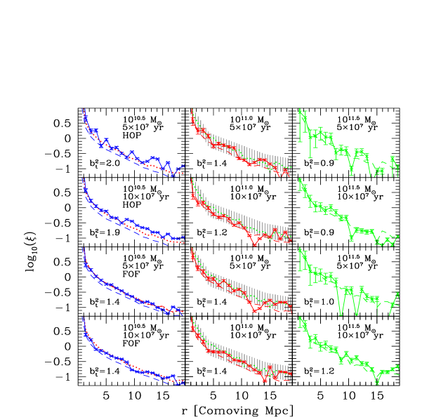
Figure 2: Spatial Correlation Functions. In each panel the dashed line shows the correlation function for all the groups, while the points connected by the solid line show $\xi(r)$ for groups that have accreted appreciable mass in the last $\Delta t$ years. Panels are labeled by their mass range and $\Delta t$ values, and in each panel, the dotted line shows the correlation function of all the groups in the next highest mass bin. The top two rows were generated from a set of groups selected by the HOP algorithm, while the groups in the lower two rows were selected using the FOF approach. The shaded region in the central panels represents the observed correlation function of ${\cal R}_{AB}\leq 25.5$ Lyman break galaxies as computed in we01 by inversion of the angular correlation function. A 10% accretion threshold is applied in the $10^{11.5}{M_{\odot}}$ case to increase the number of measured groups.

In Figure 2 we show the spatial correlation functions of the groups selected by both the HOP and FOF algorithms and compare them with $\xi(r)$ of the accreting groups. This function measures the excess probability of finding a pair of groups at a given separation $r$ relative to a random distribution, and is calculated for a separation bin $r_{l}$ as

$$1+\xi(r_{l})=N(r_{l})/N_{\rm random}(r_{l}),$$ (1)

where $N(r_{l})$ is the number of pairs separated by distances between $r_{l}$ and $r_{l+1}$, and $N_{\rm random}(r_{l})=\frac{1}{2}N^{2}\frac{4\pi}{3}({r_{l+1}^{3}-r_{l}^{3}})/V$, with $N$ the total number of groups and $V$ the volume of the simulation. In the accreting case we co-added the correlation functions calculated from the differences from the last four $\Delta t=5\times 10^{7}$ year intervals and the last two $\Delta t=10\times 10^{7}$ year intervals. Radial bins of 1/80 the simulation size, corresponding to $0.92$ comoving Mpc, were taken throughout. For comparison, in each panel of Fig. 2 we also show the correlation function of all the groups in the next largest mass bin. The amplitudes of the correlation functions obtained using the full set of HOP and FOF groups agree with each other to within statistical uncertainties, as well as with analytical estimates.

The upper row demonstrates a clear enhancement of the clustering of accreting groups at both the $10^{10.5}M_{\odot}$ and $10^{11.0}M_{\odot}$ mass scales, with their correlation functions roughly matching those of objects three times greater in mass (no conclusion can be drawn from the high mass bin as the sample is too small). This “temporal biasing” arises from the fact that both objects accreting substructure as well as those experiencing considerable smooth infall tend to be found in the densest regions of space, which are themselves highly clustered. This conclusion is supported by the fact that the average local overdensity of groups in the $10^{10.5}(10^{11})M_{\odot}$ mass bin is 0.82(0.87) (measured in 4 Mpc (comoving) spheres, corresponding to a mass scale of $1.2\times 10^{13}$ $M_{\odot}$), whereas the same mass bin for the entire population exhibits an overdensity of 0.60(0.73).

In the second row of Fig. 2 we take a longer interval of $\Delta t=10\times 10^{7}$ yr. This has a only slight dampening effect on temporal bias, which can not be definitively distinguished from statistical noise in our measurements. In the $\Delta t=20\times 10^{7}$ yr case, however, only a very weak enhancement of $\xi(r)$ was measured.

In the lower two rows of this figure, we repeat our analyses using the FOF group finder. Although this approach is more susceptible to statistical noise, the same trends are apparent as in the HOP case. If $\Delta t=5\times 10^{7}$ yr, this temporal bias is roughly equal to the geometrical bias of the groups three times more massive, while if $\Delta t=10\times 10^{7}$ yr, $\xi(r)$ is boosted to a slightly lesser degree.

Finally, to quantify our results, we have computed the effective temporal bias in each mass bin, $\Delta t$, and group finder. We define $b^{2}_{t}$ as the ratio of the correlation function of the accreting groups to the overall correlation function, weighted by the number of points in each bin in the overall function; $b^{2}_{t}\equiv\sum^{20}_{i=0}\frac{\xi_{{\rm accreting},i}N_{{\rm all},i}}{\xi_{{\rm all},i}N_{{\rm all},i}}$, where the sum is carried out over all bins within $r\leq 20$ comoving Mpc. These values are labeled in each panel, and in the $\Delta t=20\times 10^{7}$ yr case, $b^{2}_{t}=$ 1.1(1.0) in the $10^{10.5}(10^{11.0}){M_{\odot}}$ HOP bins and 1.1(1.3) in the respective FOF bins.

IV Astrophysical Implications

While temporal bias is a general property of the peaks of a gravitationally amplified Gaussian random field, our results have specific implications for the large sample of $z\sim 3$ galaxies made available by the Lyman-break color-selection technique st98 . Lyman break galaxies (LBGs) are observed to have enormous star-formation rates on the order of $\sim 50{M_{\odot}}$ per year ad00 , implying that these objects are likely to be accreting large amounts of material. Furthermore, although the clustering of LBGs brighter than ${\cal R}_{AB}\leq 25.5$ is roughly that expected from the geometrical bias of $10^{12}{M_{\odot}}$ objects [e.g. 16, 17], the linewidths measured from a spectroscopic sample these galaxies correspond to total masses $\leq 10^{11}M_{\odot}$ pe01 .

To relate our result to LBGs we plot the spatial correlation function of ${\cal R}_{AB}\leq 25.5$ LBGs, as derived in we01 , in the center column of Fig. 2. Although there are significant uncertainties involved in computing this quantity, since comparisons are more naturally conducted in angular coordinates, the shaded regions provide a guide to the range of $\xi(r)$ values consistent with observations. In these panels, we see that if $\Delta t=5\times 10^{7}$ yr is chosen, then temporal bias boosts the correlation function of $10^{11}{M_{\odot}}$ groups into reasonable agreement with observations.

This mass is marginally consistent with the upper mass bound inferred from the rotation curves of a somewhat bright (${\cal R}_{AB}\lesssim 24$) spectroscopic subset of LBGs pe01 . Furthermore, only $\sim 4\%$ of all groups exhibit appreciable accretion in each $\Delta t=5\times 10^{7}$ year time interval and the density of $10^{11}{M_{\odot}}$ groups is $\sim 2\times 10^{-2}$ Mpc³, at $z=3$ in our assumed cosmology. Thus associating such objects with $5\times 10^{7}$ year starbursts results in a density $\sim 5\times 10^{-4}$ Mpc³, comparable with that observed.

While quite suggestive, these comparisons are not meant as a complete model, and may not prove to be the final explanation of the discrepant mass estimates of LBGs. Kinematic models have been explored, for example, in which the observed velocity dispersions of LBGs are much less than the circular velocities of the groups in which they are contained mo99 . What is clear however, is that this bias can not be ignored and must be carefully considered when interpreting the clustering of these objects. While perhaps only part of the story, temporal biasing represents an important factor that must be taken into account when studying the properties of Lyman break galaxies.

- (1) Linde, A. D. 1983, Phys. Lett., 129B, 177
- (2) Eke, V. R., Cole, S., & Frenk C. S. 1996, Monthly Notices of the Royal Astronomical Society, 282, 263
- (3) Kaiser, N. 1984, Astrophysical Journal, 284, L9
- (4) Mo, H. J. & White S. D. M., 1996, Monthly Notices of the Royal Astronomical Society, 282, 348
- (5) Jing, Y. P. 1999, Astrophysical Journal, 515, L45
- (6) Scannapieco, E. & Thacker, R. J. 2003, Astrophysical Journal Letters 590, 69
- (7) Spergel, D. N. et al. 2003, Astrophysical Journal Supplement, 148, 175
- (8) Perlmutter, S. et al. 1999, Astrophysical Journal, 517, 565
- (9) Couchman, H. M. P., Thomas, P. A., & Pearce, F. R. 1995, Astrophysical Journal, 452, 797
- (10) Thacker, R. J & Couchman, H .M. P. 2000, Astrophysical Journal, 545, 728
- (11) Davis, M., Efstathiou, G., Frenk, C. S., & White, S. D. M. 1985, Astrophysical Journal, 292, 371
- (12) Eisenstein, D. J. & Hut, P. 1998, Astrophysical Journal, 498, 137
- (13) Percival, W. J., Scott, D., Peacock, J., A., & Dunlop, J. S. 2003, Monthly Notices of the Royal Astronomical Society, 338, L31
- (14) Steidel, C. C., Adelberger, K. L., Dickinson, M., Giavalisco, M., Pettini, M., Kellogg, M. 1998, Astrophysical Journal, 492, 428
- (15) Adelberger, K. L. & Steidel, C. C. 2000, Astrophysical Journal, 544, 218
- (16) Wechsler, R. H., Somerville, R. S., Bullock, J. S.; Kolatt, T. S.; Primack, J. R.; Blumenthal, G. R.; Dekel, A. 2001, Astrophysical Journal, 554, 85
- (17) Porciani, C. & Giavalisco, M. 2002, Astrophysical Journal, 565, 24
- (18) Pettini, M et al. 2001, Astrophysical Journal, 554, 981
- (19) Mo, H. J., Mao, S., & White, S. D. M. 1999, Monthly Notices of the Royal Astronomical Society, 304, 175