Star Clusters in Virgo and Fornax Dwarf Irregular Galaxies

Abstract

We present the results of a search for clusters in dwarf irregular galaxies in the Virgo and Fornax Cluster using HST WFPC2 snapshot data. The galaxy sample includes 28 galaxies, 11 of which are confirmed members of the Virgo and Fornax clusters. In the 11 confirmed members, we detect 237 cluster candidates and determine their V magnitudes, V-I colors and core radii. After statistical subtraction of background galaxies and foreground stars, most of the cluster candidates have V-I colors of -0.2 and 1.4, V magnitudes lying between 20 and 25th magnitude and core radii between 0 and 6 pc. Using H$\alpha$ observations, we find that 26% of the blue cluster candidates are most likely HII regions. The rest of the cluster candidates are most likely massive ($>$10⁴ M_⊙) young and old clusters. A comparison between the red cluster candidates in our sample and the Milky Way globular clusters shows that they have similar luminosity distributions, but that the red cluster candidates typically have larger core radii. Assuming that the red cluster candidates are in fact globular clusters, we derive specific frequencies (S_N) ranging from $\sim$0-9 for the galaxies. Although the values are uncertain, seven of the galaxies appear to have specific frequencies greater than 2. These values are more typical of ellipticals and nucleated dwarf ellipticals than they are of spirals or Local Group dwarf irregulars.

1 Introduction

The study of extragalactic globular cluster systems in galaxies of a variety of Hubble types has led to the development of a number of scenarios that place globular clusters within the context of galaxy formation and evolution. Carney & Harris (2001) and van den Bergh (2000a) reviewed the myriad pieces of evidence derived from globular cluster systems and the scenarios designed to explain them. The properties of globular clusters in giant elliptical galaxies, in particular, have led to suggestions that globular cluster systems form 1) in situ, perhaps in the hierarchical collapse of the halo (Côté et al., 2000) and possibly in multiple phases (Forbes et al., 1997); 2) in galaxy mergers, both through the formation of new clusters in the colliding gas (e.g. Schweizer et al., 1996) and through the combination of the pre-existing globular cluster systems (e.g. Forbes et al., 2000); 3) by accretion of the clusters of smaller galaxies (Cote et al., 1998), as exemplified by the $\sim$4 GCs being contributed to the Milky Way (Da Costa & Armandroff, 1995) by the Sagittarius dwarf galaxy (Ibata et al., 1994). More recently the second two of these ideas have been incorporated into the current cosmological scenario using simulations (e.g. Kravtsov & Gnedin, 2003) and semi-analytic methods (e.g. Beasley et al., 2002).

The generally low globular cluster specific frequencies ($S_{N}$, the number of clusters normalized by the galaxy magnitude; Harris & van den Bergh, 1981) observed in nearby dwarf and spiral galaxies pose a difficulty for the third of the above possibilities, a point which was raised by van den Bergh (1982) in argument against spiral-spiral mergers explaining the high $S_{N}$ of cD galaxies. However, it may be misleading to compare the specific frequences of spiral and dwarf galaxies residing in nearby low-density galaxy groups with those of giant elliptical galaxies found in more distant rich clusters of galaxies, since the role of the environment in the assembly of globular cluster systems is not understood. A census of the globular cluster systems of a wide variety of galaxies drawn from the same environment is needed to properly assess the roles that each of the formation mechanisms may play.

Miller et al. (1998) embarked on such a census through the study of the globular clusters of dwarf elliptical (dE) galaxies in the Virgo, Fornax, and Leo clusters. The results of that survey revealed a distinction between the globular cluster populations of nucleated dE (dE,N) and nonnucleated dE galaxies; in particular, dE,N galaxies were found to have a factor of 3 higher $S_{N}$ than nonnucelated dEs. The high $S_{N}$ of dE,N align them more closely with giant elliptical galaxies than with dwarf irregular (dIrr) and spiral galaxies, which from measurements in local galaxies have $S_{N}\sim 0.5$ (Harris, 1991); the nonnucleated dE’s, on the other hand, do have $S_{N}$ that resemble those of dIrrs and spiral galaxies, once fading of the young stellar populations is taken into account. The difference in $S_{N}$ between dE and dE,N galaxies thus suggests globular cluster formation processes in dE,N and giant ellipticals that are different from those of spirals and dIrrs. Moreover, it argues that not all dE galaxies represent the stripped or harassed remnants of dIrr galaxies, processes described by e.g. Lin & Faber (1983) and Moore et al. (1998).

These conclusions depend, however, to large degree on the validity of comparing globular cluster populations in rich-cluster dE galaxies with those of local dIrr and spiral galaxies. In this paper, we discuss the results of a Hubble Space Telescope (HST) snapshot survey of dIrr galaxies in the Virgo and Fornax galaxy clusters, the same environments from which many of the dE galaxies of Miller et al. (1998) were drawn. We describe the observational sample and data reduction in §2. In §3, we describe our technique for detecting candidate globular clusters. We present the properties of our sample of candidate globular clusters, derive specific frequencies, and examine individual galaxies in §4. Some of the more interesting results are discussed in §5, followed by our conclusions in §6.

2 Observations and the Galaxy Sample

The galaxy sample, shown in Table 1, was observed as part of a snapshot program GO-7377 (PI: Miller) using the WFPC2 camera of HST. All HST observations consisted of two 240 second exposures in the F555W filter and one 300 second exposure in the F814W filter. The galaxies, which have typical sizes of $\sim$30 arcsec, were in all cases centered and completely contained (except VCC 1448) on the WF3 chip. The F555W observations, with their much more accurate cosmic ray removal, are used for most of the analysis in the paper. The F814W observations are only used to derive the V-I colors.

The HST sample originally included 29 galaxies selected from the Virgo Cluster Catalog (VCC; Binggeli et al., 1985), Fornax Cluster Catalog (FCC; Ferguson, 1989), and Dorado Group Catalog (DGC; Ferguson & Sandage, 1990) in a manner similar to that used to select the dE galaxies for Miller et al. (1998), Lotz et al. (2001), and Stiavelli et al. (2001). Targets classified as Im or dE/Im in the catalogs and that do not have HST guide stars within 3 arcminutes (so as to limit the chance of having a highly saturated star in the field) were selected. Since lower luminosity galaxies are more likely to have fewer clusters, more galaxies were selected in lower-luminosity bins. Since a minority of galaxies had measured velocities, radial velocity was not used as a selection criteria. In addition, the dI/dE transition object NGC 4286 (Sandage & Hoffman, 1991) was included as a special target because it fit a project goal of investigating the connections between dE and dI galaxies. Of these 30 galaxies 29 were observed successfully during HST Cycle 7. In this paper we concentrate on the 28 galaxies in the Virgo and Fornax cluster in this sample.

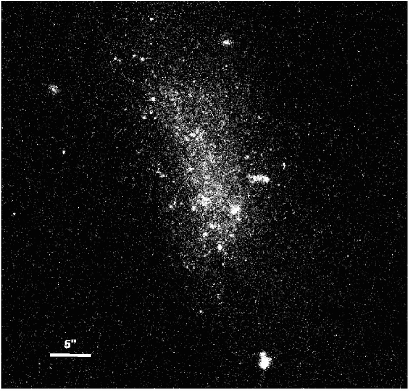
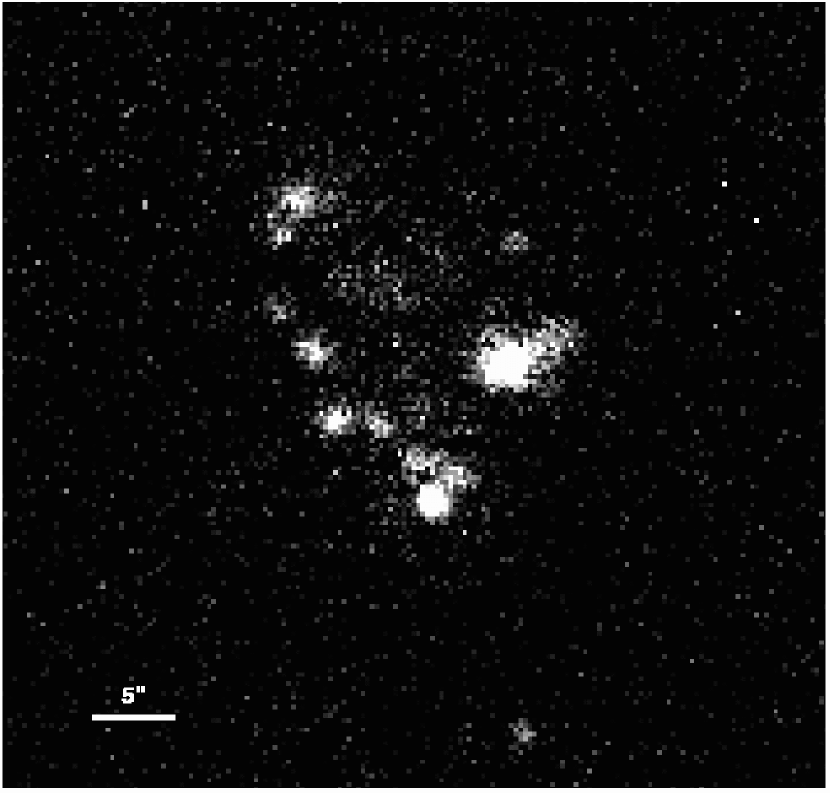
Figure 1: on the left, (1a) shows the HST image of VCC 328, while on the right (1b) shows the H$\alpha$ image of the same galaxy. The images are aligned and at the same scale.

The initial reduction procedure for the HST data was similar to that given in Miller et al. (1997). The two F555W images were combined and cleaned using IDL routines supplied by Richard White of STScI. All other processing was done using scripts written in IRAF. The cleaned F555W images were then used as templates to identify and remove cosmic rays in the F814W images. An HST image of one of the sample galaxies, VCC 328, can be seen in Figure 1a.

H$\alpha$ images were taken through a set of four narrow band (FWHM=20Å) filters on the Apache Point Observatory 3.5m telescope in April, 2003. Each galaxy was observed through an ’ON’ filter tuned to the velocity of the galaxy and an ’OFF’ filter, separated by at least 1000 km/sec from the galaxy velocity. The filters had central wavelengths of 6563, 6585, 6607 and 6629 Å. Feige 34 was used as a spectrophotmetric standard (Massey et al., 1988). Based on the scatter in the photometry of Feige 34, we estimate that absolute fluxes are only accurate to 50% due to the presence of some clouds during the first night of observations. Observations on subsequent nights allowed for the bootstrapping of the flux calibration using the galaxy VCC 1374. Bias subtraction and flat fielding were performed using CCDPROC. For one filter (centered at 6585Å), the flat fielding left 10% variations in the sky level across the field requiring the use of an illumination correction image. This illumination correction image was derived from seven program images with the sources masked using SEXtractor. After the illumination correction the sky was constant to 2%. Following flat-fielding, the sky was subtracted from each image and cosmic rays were removed using the IDL routine la_cosmic (van Dokkum, 2001). The ON and OFF images were then aligned and scaled using the brightest stars in each field and then were subtracted. The resulting H$\alpha$ images (one example is shown in Figure 1b) have detection limits corresponding to a flux of $\sim 3\times 10^{35}$ ergs/sec at a distance of 17 Mpc. To determine accurate WCS coordinates for the images, we used the IRAF MSCRED task MSCZERO (Valdes, 1997). Based on the scatter of stars relative to their expected positions within the field, these coordinates are good to within 1$\arcsec$.

3 Identifying Star Cluster Candidates

This section will detail the process by which we identify and derive properties of candidate clusters. Before explaining the process in detail, we provide a brief overview:

Using DAOPHOT II (Stetson, 1987), we derived a point-spread function (PSF) using HST data of the Large Magellanic Cloud (LMC) cluster NGC 1868. We convolved this PSF with King profiles of varying size to create model cluster profiles. Then for each of the galaxies in our sample, sources were identified and fit to the model cluster profiles to determine their magnitudes and sizes. To obtain a list of candidate star clusters in each galaxy, we assumed that all point-like sources on the WF3 chip between our completeness limit and an M_V of -11.5 are potential clusters. We then used the flanking WF2 and WF4 chips on the WFPC2 camera to correct for the presence of background galaxies and foreground stars in our list of cluster candidates.

An alternate method for finding cluster candidates in nearby, late-type, external galaxies with HST data is given by Dolphin & Kennicutt (2002). The methods are similar in that both detect magnitudes and sizes for cluster candidates in galaxies at moderate distance, but differ in the method used to determine those quantities, and the way in which the cluster samples are defined.

For simplicity, throughout the paper we assume a distance to Virgo and Fornax of 17 Mpc (DM of 31.15) consistent with the distances given in Ferrarese et al. (1996) and Silbermann et al. (1999). Differences in the distance modulus of a few tenths of a magnitude should not strongly affect our results.

3.1 Determining the PSF

To determine a PSF for the WF2, WF3 and WF4 chips in the F555W filter we used WFPC2 observations of a field of the LMC cluster NGC 1868 that were taken on Nov. 12, 1998 – close in time to the majority of our observations (see Table 1). The PSFs were characterized in DAOPHOT II using roughly 100 stars distributed across each chip. The derived PSFs (one for each chip) are a position dependent combination of a Moffat function with $\beta$=1.5 and sub-pixel corrections. The PSF was fit using a 5 pixel (0.5 arcsec) radius and extends over a 7 pixel radius. We conducted a qualitative test comparing our derived PSFs to Tiny Tim PSFs (Krist, 1995) by subtracting both from point-source fields (using SUBSTAR in DAOPHOT II) and found that our derived PSFs left behind much less residual flux. We will discuss results on the stability of the PSF in the next section.

Because we are interested in determining the radii of the star cluster candidates, we created model cluster profiles by convolving the derived PSF with King profiles. Seventeen different King profiles were used, all with a tidal radius of 40 pc, a value typical of Galactic globular clusters (Harris, 1996), and a core-radius of 0 (the original PSF), 0.25, 0.5, 0.75, 1, 2, 3, 4, 5, 6, 7, 8, 10, 12, 15 and 20 pc (where all physical sizes assume a distance of 17 Mpc). The model cluster profiles are always referred to by their physical sizes; note that 1 WFPC2/WF pixel = 0.1 arcsec = 8.2 pc at 17 Mpc. The convolution of the PSF with the King profiles was done in IDL at 5 times the pixel resolution in order to avoid the effects of undersampling. The model cluster profiles were then converted back into DAOPHOT’s PSF format, with a lookup table for the variation of the PSF as a function of position in the frame and its sub-pixel position.

3.2 Photometry and Radii Determination

A pipeline consisting of DAOPHOT II and IDL programs was used to identify candidate clusters. Sources were found using the DAOPHOT II FIND routine using a threshold of 5$\sigma$ and a FWHM of 1.4 pixels. Lower thresholds were found to give too many spurious sources. Changing the FWHM was found not to strongly affect the number/quality of detected sources - partially resolved (broader) sources were not thrown out by the routine. However, asymmetric sources are rejected by the FIND routine, perhaps resulting in the elimination of some larger HII regions from our sample.

Aperture photometry was then done using the PHOT routine with a 5 pixel / 0.5 arcsec radius, which is the radius at which the WFPC2 standard photometric system is defined (Holtzman et al., 1995). For the profile photometry, we fit each source in the F555W images to all 17 of the model cluster profiles in turn (see §3.1). For most sources, the $\chi$ (the quality-of-fit parameter output by DAOPHOT II) of the profile fit varies smoothly with the core radius of the model cluster profile. This is shown for a number of sources in VCC 1448 in Figure 2. Note that many of the minimum $\chi$ values have values very close to 1, confirming that the PSF and model cluster profiles accurately match the data. The fit with the minimum $\chi$ value was used to derive photometry and to determine the core radii of the cluster candidates. Aperture corrections were measured for each of the model cluster profiles and ranged between +0.026 for the more compact model cluster profiles and +0.034 for the model cluster profile with R_core=20pc. Since the majority of our cluster candidates have R${}_{core}<5$pc, we applied an aperture correction of +0.026 to all data. Figure 3 shows the scatter in profile-fit and aperture photometry. The scatter shows an asymmetric distribution with the aperture photometry in general being brighter, probably due to confusion from background and nearby sources. In our final sample (crosses), this scatter is significantly reduced due by our application of a 90% completeness cut (see §3.4) and the exclusion of two high surface brightness regions in VCC 1374.

For both aperture and profile-fit photometry the F555W and F814W fluxes were converted into Johnson V and Kron-Cousins I magnitudes using the procedure given in Holtzman et al. (1995). In addition, the charge transfer efficiency was corrected for using the method in Stetson (1998) and the geometric distortion was corrected for by multiplying the images by the pixel area map. The V magnitudes of all sources were derived from the profile-fit photometry (V_profile); however, we don’t derive F814W profile-fit photometry and so aperture magnitudes (for both V & I) are used for colors. The median error on the V-I color is 0.15 magnitudes for our full sample of cluster candidates. In the color range between V-I of 0.5 and 1.5, critical for separating young and old clusters, the median V-I error is 0.12 magnitudes. These errors are derived from the errors in the aperture magnitude as reported by DAOPHOT II.

Magnitudes for the galaxies as a whole were also derived from the WFPC2 F555W data. The magnitudes were calculated in two ways: (1) by computing the total flux within a circular aperture with a radius two times the pertrosian radius (Petrosian, 1976), and (2) by summing up all the light in the WF3 chip after masking out clearly extended background galaxies and very bright foreground stars. We take the mean of these two methods as the galaxy magnitude, V_T, shown in Table 2. Also shown is the difference in the two magnitudes, $\Delta$V_T. This number, which is larger than the formal error in the magnitude calculation, gives a sense of the uncertainty in our magnitudes. For brighter galaxies this difference is typically less than 0.1 magnitudes, while it is over 1 magnitude for the faintest galaxies in our sample. No color or CTE corrections were made to the magnitudes, these effects contribute to V_T below the 0.1 magnitude level. As noted earlier, VCC 1448 is larger than the WF3 chip field of view, and FCC 76 and VCC 888 also may contain some emission off the chip; for these galaxies, the magnitudes given are lower limits.

As noted above, a measure of the core radius of each candidate cluster is obtained using the best fitting model cluster profile. At our assumed distance of 17 Mpc, one WF pixel corresponds to 8.2 pc. We expect to be able to determine core radii smaller than this, because the broadening due to the King profiles extends out past the central pixel; for example, the fraction of light falling outside of the central pixel changes from 63% for the PSF to 79% for the model cluster profile with a core radius of 2 pc. Nevertheless, it is important to consider the effects of our limited spatial resolution and of the variability in the $HST$ PSF on our measurements of the core radii of cluster candidates. We address the issue of the constancy of the PSF here, and address the effects of resolution and random error in the next section.

We conducted a test to check whether or not our routine accurately detected point-sources in seven WFPC2 fields taken during the period Aug. 2, 1997 to Apr. 3, 1999, spanning the dates of our observations. The fields were drawn from HST program PIDs 6364, 6804, 7307, 7335, and 7434. All fields were either Galactic globular clusters or located in the Large Magellanic Cloud and thus should be dominated by point sources. We ran them through the same pipeline as we used for our program sources. Including all seven fields, $\sim$80% of the isolated sources were best fit by model cluster profiles with core radii less than or equal to 1 pc (0.012 arcsec). As a comparison, only $\sim$40% of isolated sources in our program sources were best fit by model cluster profiles with core radii $\leq$ 1 pc. This test shows that our method reliably assigns point sources small values for the core radius. It also allows us to examine the variation of the PSF over time, which would result in a systematic error in our determinations of the cluster radii. For the seven fields, the peak in the best-fitting core radius distribution varied between 0 and 1 pc. This suggests that the PSF is unstable at a level corresponding to $\sim$1 pc (0.012 arcsec) in our method. As we will see in the next section, this is roughly the same level as our random error on a single measurement of the core radius.

3.3 Artificial Star/Cluster Tests

We conducted artificial star and cluster tests using the DAOPHOT II ADDSTAR routine. These tests were done by adding grids of objects generated from the original PSF (R_core=0 pc) and model cluster profiles with R_core of 1, 3, 7 and 12 pc. The grids were added to the WF3 chip galaxy images with a random position offset and typically contained 600 objects each separated by 30 pixels. Input magnitudes for the stars were determined randomly and ranged from 18th to 27th magnitude. The fields with the added stars/clusters were then run through the same pipeline outlined in the previous section to identify and determine properties of the objects. Because identification and determination of the radius was done using the F555W observations, the tests were only done for those images. For each galaxy, a minimum of 50,000 artificial objects were inserted for each of the five model cluster profiles used. The artificial star and cluster tests were run using the Condor distributed computing software.

Curves of fifty and ninety percent completeness as functions of R_core and F555W magnitude are shown in Figure 4a. The completeness is best for point sources and gets worse with increasing core radius due to the broader profiles and lower surface brightnesses of these objects. This result is generally applicable to all surveys of extragalactic globular clusters – the completeness limit for point sources can differ by more than a magnitude from the completeness limit of more extended objects. This makes correcting for this completeness function complicated if there are large numbers of extended sources. We note that the F555W magnitudes differ from the Johnson V magnitudes by a color correction term which is typically small (few $\times 10^{-2}$ magnitudes), and therefore can be ignored for the completeness limits. The derived error on the magnitudes is typically $<$0.01 on the bright end and $\sim$0.2 near the 50% completeness limit. Our actual errors, especially on the bright end, will be somewhat worse than this due to the effects of pixelization.

The artificial cluster tests can also be used to determine the random error in our determination of the core radii of the cluster candidates. Figure 4b shows the standard deviation of the difference between the input core radius and the detected core radius ($\sigma$(R_core)). For point sources, this number is typically less than 1 pc, consistent with the results from our point source fields test. Most of the galaxies have similar errors at each core radius, but the brightest galaxies have larger errors caused by the increased background against which the profiles were fitted. The error in core radius also is a function of magnitude - the median value of $\sigma$(R_core) is shown for each input core radius in Figure 5. The vertical lines indicate the median 90% completeness for each input core radius.

Given the systematic error of up to 1 pc from the point source fields test, and the random errors shown in Figure 4b and Figure 5, we believe our measurements of core radius have an error of $\sim$2 pc for objects brighter than the 90% completeness limit. In addition, the decreased random error for small objects means that objects with a best-fitting core radius of $\geq$2 pc can reliably be considered resolved.

3.4 Defining the Sample

In this section, we describe how we defined a sample of candidate clusters based on their individual properties and then how we statistically corrected that sample in order to determine the number of clusters in each galaxy.

We defined the sample of candidate clusters conservatively. Using the completeness data above, we interpolated the 90% completeness function for each galaxy to all core radii and used only clusters brighter than this limit. The limit corresponded to a V_profile between 24.15 and 24.55 (M_V of -7.0 to -6.6), and was chosen to ensure the accuracy of the measured properties of the cluster candidates. Clusters brighter than V_profile=19.65 (M_V=-11.5) were also rejected. This limit on bright objects was chosen to include even the brightest globular clusters. It should also include all but the most massive young clusters (e.g. all the young and old clusters in the LMC would be included). The final number of cluster candidates in each galaxy is shown in Table 2.

It is important to consider the possible sources of contamination in our sample.

1. Background galaxies - especially compact ellipticals and bulge components of spiral galaxies.

2. Foreground stars - faint stars in our own Galaxy.

3. Compact, symmetrical HII regions in the target galaxies.

4. Single, very bright stars in the target galaxies.

5. Spurious detections in high surface brightness regions with many overlapping sources.

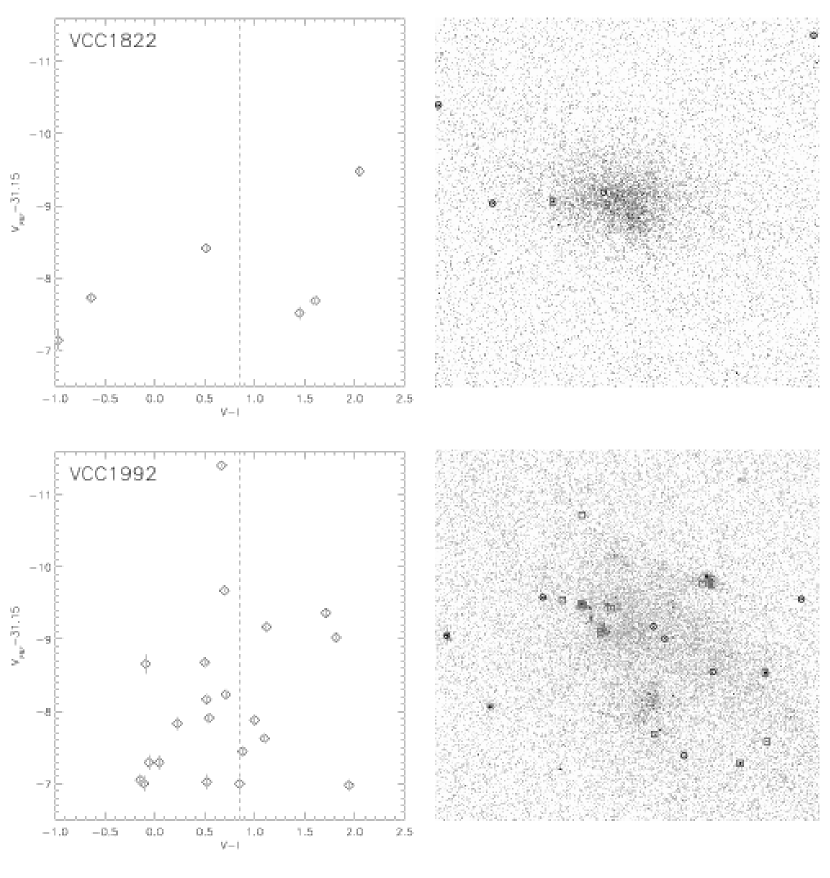
Figure 14: Left – Color magnitude diagram of all cluster candidates. The dashed line at V-I=0.85 represents the dividing line between red and blue CCs. Right – F555W band images of the WF3 chip for each galaxy. Red cluster candidates are shown as circles while blue cluster candidates are denoted with squares.

Visually examining the data, only one of our galaxies (VCC 1374) contained problematically high surface brightness regions. The sources detected inside two high surface brightness regions in that galaxy were removed from the sample. These two regions can be clearly seen in Figure 14 outlined by white boxes. The contamination of the sample by extremely bright stars was minimized by our inclusion of only those objects brighter than M${}_{\rm V}\sim-7$. Contamination of our sample by compact HII regions will be examined later using the H$\alpha$ data in a subsample of the galaxies.

We obtained background and foreground (BG/FG) source counts from the flanking (WF2 and WF4) fields. In this section we describe how we found the expected BG/FG level for each galaxy. The expected BG/FG levels are then used in two ways: (1) to remove the BG/FG sources from the sample of candidate clusters as a whole, described in §4, and (2) to determine the number of red candidate clusters in each galaxy for use in computing individual specific frequencies as described in §4.1.

We based the expected BG/FG level on the mean level of sources in the flanking fields in the entire sample. However, because each galaxy has different completeness limits, the BG/FG level varies from galaxy to galaxy. To determine the BG/FG level in a specific galaxy, all the sources in the flanking fields were put through the 90% completeness cut and bright-end V${}_{\rm profile}>$19.65 cut as described earlier in this section. Then the BG/FG level and error were determined by taking the mean and standard deviation of the number of remaining sources in each flanking field. The values for each galaxy are shown in Table 2. Note that the number of cluster candidates in Table 2 is not corrected for the BG/FG level in any way. We also note that because the Virgo and Fornax fields had nearly identical average BG/FG counts and standard deviations, all fields were used in the BG/FG level determination.

Figure 6 shows the number of candidate clusters vs. the number of BG/FG sources on each chip. About half of all the galaxies, and 9 of the 11 galaxies with confirmed cluster membership, appear to have significant number of candidate clusters. The remaining galaxies have a number of candidate clusters consistent with the BG/FG contamination level.

We note that in the tables, figures, and analysis that follow we excluded the eight candidate clusters with R_core values of 20pc. These objects were either the bulges of obvious background galaxies, or were in highly confused regions and most likely have inaccurate sizes, magnitudes and colors.

3.5 H$\alpha$ Observations

For the seven galaxies that are confirmed members of the Virgo cluster we have deep H$\alpha$ observations. The reduction of these data was described in §2. The H$\alpha$ data were used to find the galaxy-wide H$\alpha$ flux assuming a distance of 17 Mpc (Table 3). From the H$\alpha$ fluxes, we derived star formation rates using the relationship given by Kennicutt et al. (1994):

$$SFR[\frac{M_{\odot}}{yr}]=\frac{L_{H\alpha}}{1.25\times 10^{41}[ergs/sec]}10^{0.4A_{H\alpha}}$$ (1)

where $L_{\rm H\alpha}$ is the H$\alpha$ luminosity and $A_{\rm H\alpha}$ is the absorption by dust at H$\alpha$ (0.78 A_V). The values for the star formation rates given in Table 3 were calculated assuming no extinction by dust internal to the galaxies and are thus lower limits. Assuming absorption similar to that of hot stars in the LMC, $A_{\rm H\alpha}\sim 0.3$ (Zaritsky, 1999), neglecting extinction would make the SFRs in Table 3 roughly 30% too small. Note that the H$\alpha$ fluxes and SFRs in Table 3 have errors dominated by the absolute calibration of the photometry (i.e. 50%). The H$\alpha$ fluxes are in rough agreement with those given in Heller et al. (1999) for VCC 328, 1374 and 1992. The largest difference is for VCC 1374, where our flux is roughly a factor of two (2$\sigma$) smaller than in Heller et al. (1999). We also detect H$\alpha$ in VCC 1822 where they had a just an upper limit of $\sim 10^{38}$ ergs/sec. The values found for star formation rates fall in the same range as the dwarf irregulars in the Local Group (Mateo, 1998).

As mentioned in §3.4 compact HII regions are one possible source of contamination in our sample. To determine the possible contamination of clusters by HII regions, we first measured the H$\alpha$ flux in a 1$\arcsec$ annulus around the location of each cluster. Then, using a Balmer decrement of 2.8 (Osterbrock, 1989) and the WFPC2/F555W filter transmission curve ($\sim$7.5% at H$\beta$ and $\sim$1.3% at H$\alpha$) we calculated the contribution of the H$\alpha$ and H$\beta$ line flux to the V-band magnitude, V_Hα. The relation between this derived magnitude and the actual contribution to the F555W flux is somewhat uncertain due to three effects: (1) the absolute calibration of the H$\alpha$ is reliable only to about 50%, (2) any dust will reduce the H$\beta$ flux relative to the H$\alpha$ flux and (3) the poorer resolution of the ground based H$\alpha$ data means that any H$\alpha$ flux located within 1$\arcsec$ of the cluster candidate will be included in our value for V_Hα. Taking into account our errors, we considered a cluster candidate a possible HII region contaminant if it had a V_Hα brighter than, or within 0.5 magnitudes of, its V_profile. Our detection limit of $\sim 3\times 10^{35}$ ergs/sec results in V_Hα $\sim$ 26, and is therefore sensitive enough to detect contamination in even our faintest sources. Only 32 out of 185 cluster candidates were found to be contaminated by H$\alpha$ emission, with 27 of those lying in the two galaxies brightest in H$\alpha$, VCC 1992 and VCC 1374. Figure 7 shows the properties of the H$\alpha$-contaminated candidate clusters. Of the blue cluster candidates (V-I $<$ 0.85), $\sim$26% were found to be likely HII regions, while only 5 (6%) of the red candidate clusters were contaminated by H$\alpha$, all located in VCC 1374. This difference between blue and red cluster candidates is not surprising, since HII regions are expected to appear blue through the F555W and F814W filters. This suggests that our sample of red clusters, which we consider to be candidate globular clusters, are essentially uncontaminated by HII regions.

4 Properties of the Cluster Sample

Of our galaxy sample, only 11 galaxies, 7 in Virgo and 4 in Fornax, have known velocities that are less than 3000  km s^-1 (see Table 1). These are the only galaxies for which cluster membership is confirmed and therefore to which the distance is known. We note that most of the other galaxies in our sample (including three VCC galaxies with high velocities) have insignficant or barely significant numbers of candidate clusters, as might be expected for more distant galaxies with fainter globular cluster systems, or for fainter galaxies within the Virgo and Fornax groups. In this section, we consider the bulk properties of the cluster candidates using only the 11 likely cluster members, FCC 76, 120, 247 and 282 and VCC 83, 888, 1374, 1448, 1822 and 1992. These 11 galaxies contain 237 cluster candidates and an expected BG/FG contamination (see Table 2) of 51 sources.

Figure 8 shows the properties of the candidate clusters before (thin) and after subtraction of the BG/FG (thick). This subtraction was done by selecting the number of expected background sources at random from the BG/FG population and then removing the closest matching cluster candidate (from the sample as a whole) in V_profile, V-I and R_core. Error bars on the histograms of the subtracted sources were determined by taking the standard deviation of 200 Monte Carlo simulations in which the candidate cluster list and the BG/FG list were drawn at random from the initial sample. The most notable difference between the BG/FG sources and the candidate clusters is in color - the BG/FG are mostly red objects, and account for almost all of the candidate clusters with colors of V-I $>$ 1.6. The BG/FG also contains many compact (R${}_{\rm core}<1$ pc) objects, as would be expected from foreground stars. The distribution of cluster candidates peaks at V-I $\sim$ 1 and R${}_{\rm core}\sim$ 0. The leftmost bin in V_profile ($>$ 24 mag) is strongly affected by our completeness-based cuts and therefore the apparent turnover at faint magnitudes is not significant. However, a turnover at that magnitude would be expected for the typical globular cluster system with M${}_{\rm V,peak}\simeq$-7.4.

We can divide the sample based on color to attempt to separate old from young clusters. The single stellar population (SSP) models of Girardi et al. (2000) show that, for any metallicity, clusters with V-I of $>$ 0.85 are likely to be older than 10⁹ years, while clusters bluer than this are likely to be younger. Using this cut, we regard the redder/older clusters as globular cluster candidates. Even if we are detecting clusters with ages of a few billion years, with our magnitude cutoff (M${}_{\rm V}\lesssim-7$) these clusters will have globular cluster masses. The bluer objects are most likely young open or massive clusters, with a small fraction being HII regions (see above). Table 3 gives the numbers of blue and red cluster candidates in each galaxy, while Figure 9 shows histograms comparing the magnitudes and sizes of all 114 blue (thick) and 72 red (thin) cluster candidates left after BG/FG subtraction. The blue objects tend to be dimmer and more compact than the red objects. This result can be explained by either the presence of single bright stars or compact open clusters among the blue cluster candidates.

Figure 10 shows the radial distribution of the blue vs. red cluster candidates after BG/FG subtraction. The red cluster candidates typically lie farther from the center of the galaxy than the blue cluster candidates. K-S tests show that the distributions are significantly different, with P values ranging between 10^-5 and 10^-3 depending on the background subtraction. This distribution is what would be expected if the red cluster candidates are an extended population of globular clusters while the blue cluster candidates are younger clusters formed in the body of the galaxy.

The color and magnitude information also allows us to roughly approximate the masses of our candidate clusters. Figure 11 shows a color-magnitude diagram of background-subtracted cluster candidates with lines representing the color-magnitude evolution of single stellar populations of three masses (Girardi et al., 2000) ranging in ages between 60 Myr and 18 Gyr. The blue clusters almost entirely lie inbetween masses of 10⁴ and 10⁵ M_⊙, while the redder clusters all have masses significantly greater than 10⁵ M_⊙, and thus do represent objects with masses similar to those of globular clusters.

The Milky Way globular cluster system (MWGCS) (Harris, 1996, revised 2003) provides a useful point of reference with which to compare our globular cluster candidates. In order to facilitate this comparison, we took the Harris (1996) catalog data and passed it through our completeness-based cuts (see §3.4) assuming a distance modulus of 31.15. Of the 141 clusters with M_V and R_core measurements in the catalog, 83 survived the cuts. Of the 96 that also had V-I color information, 76 survived the cuts. We then compared the surviving Milky Way clusters to our BG/FG subtracted sample of candidate clusters. Figure 12 shows histograms comparing the V magnitudes, V-I colors and R_core of the MWGCS to the 72 cluster candidates with V-I $>$ 0.85. These plots exhibit some notable similarities and differences between our red cluster candidates and the MWGCS.

First, the luminosity function of the red cluster candidates is similar to that of the MWGCS, with a K-S P=0.68. This indicates that the luminosity function of the red candidate clusters is consistent with the ’Universal’ globular cluster luminosity function found in other galaxies (Ashman & Zepf, 1998). This similarity also supports the idea that our red candidate clusters are, in fact, globular clusters.

Second, we consider the color distribution. The MWGCS V-I distribution is shown both before and after subtraction of the foreground reddening, where E(V-I)$=1.35$ E(B-V) (Cardelli et al., 1989). In both cases, there is a clear color cut off at V-I $\sim$ 0.8, similar to the color cut we used to select our candidate clusters. All the galaxies in our sample have foreground reddenings E(B-V) $<$ 0.04 (Schlegel et al., 1998), with an average of E(B-V) = 0.022. However, the internal reddening due to dust is likely to be larger for clusters seen inside / behind the body of the galaxy. Corrected only for the mean foreground reddening, the median color of our sample is V-I $=1.00$, corresponding to an [Fe/H] of -1.2 using the relation from Kundu & Whitmore (1998). This median color is redder than the 0.91 of the dereddened MWGCS, but is less than the average V-I of 1.04 for elliptical galaxies (Kundu & Whitmore, 2001). The median color is also redder than the globular cluster systems in Virgo, Fornax and Leo cluster dwarf elliptical galaxies (Lotz, 2003), which are found to have a correlation between host galaxy luminosity and redder colors / higher metallicity. The unknown internal reddening prevents us from determining if their is a similar correlation in our galaxy sample. Because of the unknown reddening, our median color is a redward limit and the metallicity estimate is an upper limit. This suggests that the clusters in the dwarf galaxies in our sample are in general metal-poor.

Finally, the bottom panel of Figure 12 shows that the distribution of core radii of the red cluster candidates appears to be broader than that of the MWGCS. However, errors in the determination of the core-radius could make the distribution appear broader than it is. To compensate for this, we took the detected Milky Way clusters and added to each a random error, the magnitude of which was determined by its core radius. This error was interpolated from the median of the errors shown in Figure 4b. A K-S test was performed using the resulting distribution of Milky Way core radii and that of the Virgo/Fornax red cluster candidates. The random errors applied to the Milky Way data resulted in a range of P values with a median value of 0.002 and a standard deviation of 0.009. This test confirms that the red cluster candidates are significantly broader than the Milky Way globular clusters. Note that the varying completeness limit inhibits our ability to detect broader clusters relative to more compact ones, adding to the significance of the difference between the cluster candidates and the MWGCS.

To summarize, comparison of cluster candidates with V-I $>$ 0.85 to Milky Way globular clusters suggests that their luminosity functions are similar, while the red cluster candidates have larger sizes. The average color is uncertain due to unknown reddening, but is consistent with the red cluster candidates being relatively metal poor.

4.1 Specific Frequencies

As discussed above, the number of red (V-I $>$ 0.85) cluster candidates, when corrected for the expected BG/FG level, provide an estimate of the number of globular clusters in each galaxy in our sample. A common way of expressing the number of clusters in a galaxy relative to its luminosity is the quantity S_N, the specific frequency (Harris & van den Bergh, 1981). The specific frequency is defined as:

$${\rm S_{N}=N_{GC}10^{0.4({M_{V}+15})}}$$ (2)

where N_GC is the number of globular clusters in a galaxy that has absolute magnitude M_V.

In order to determine an accurate value for the specific frequency we need to: (1) remove the BG/FG contamination from our number of red candidate clusters, (2) correct for the unobserved portion of the luminosity function, and (3) correct for the incompleteness in our sample. We remove the expected BG/FG level from our red cluster candidate count in a fairly simple way. Of all the BG/FG sources, 75% of them have V-I $>$ 0.85. Therefore we subtracted the expected number of red BG/FG sources (75% of the number given in Table 2) from the number of red candidate clusters (Table 3) to obtain N_GC. Using this value for N_GC we derived a conservative estimate of the specific frequency, shown as S_N,min in Table 3. We consider this estimate conservative because it is uncorrected for both steps (2) and (3) above.

Traditionally, S_N values are corrected for any unobserved portion of the globular cluster luminosity function. Given a Milky Way globular cluster luminosity function, with M_V,peak=-7.33 and $\sigma$=1.23 (Ashman & Zepf, 1998), we determined the fraction of sources fainter than the 90% completeness limit for point sources in each galaxy, and then scaled up N_GC by this factor. The resulting luminosity function corrections have values of $\sim$1.4. These corrections and the specific frequencies calculated with them (“S_N w/ Corr”) are shown in Table 3 and plotted in Figure 13.

We are unable to correct for the incompleteness in our data because the incompleteness is dependent on the unknown size distribution of the clusters. However, given that most of our sources are fairly compact, and that we define our sample using only clusters brighter than the 90% completeness level, the correction for incompleteness should be small.

In both S_N calculations, M_V was derived from the magnitude in Table 2 assuming a distance modulus of 31.15; the error in the bars include the effects of Poisson noise, the errors in the BG/FG counts and galaxy magnitudes ($\Delta$V_T in Table 2), and uncertainty introduced by the errors in the V-I colors.

Our calculated specific frequencies may be in error due to the following effects: (1) Internal reddening in the galaxies can cause some young clusters to have colors that would land them in our red sample. This would result in an overestimate of the specific frequency. Given the low star formation rates of most of our galaxies, it is unlikely that there are large numbers of young embedded clusters in our sample. Such clusters might also be expected to be associated with H$\alpha$ emission. Of the seven galaxies in our H$\alpha$ sample, only one (VCC 1374) had any red clusters associated with H$\alpha$ emission. The effect of the random errors in V-I color on the specific frequency are included in the error estimates given in Table 3 and Figure 13. (2) The lack of a completeness correction. In both estimates of the specific frequency given above, we are unable to correct for the possible presence of faint, extended objects. This could result in an underestimate of the specific frequency. (3) In order to compare our S_N values with those of early-type galaxies it is traditional to “age-fade” the magnitude of the galaxies to the magnitude it would have if it were an old stellar population (Carney & Harris, 2001, p. 310). Using a scenario in which a galaxy forms stars at a constant rate for 5 Gyr and then fades for 5 Gyr, Miller et al. (1998) find a fading of $\sim$1.5 magnitudes in V, resulting in factor of $\sim$4 increase in specific frequencies. However, without better knowledge of the stellar populations of the galaxies, and the destruction timescales for the globular clusters, it is not possible to determine what the exact increase in specific frequency would be. (4) Intermediate-age ($>1$ Gyr) massive clusters may be included in this sample. To get a sense of the number of intermediate age clusters we might be detecting, we used the LMC as a case study. The LMC provides a nearby laboratory in which cluster ages are well known. Using the old and intermediate-age LMC clusters given in (Geisler et al., 1997) and our detection limits, we would detect $\sim$10 clusters as red candidate clusters. Only half of these are bona fide globular clusters, with the other half being clusters with ages of a few gigayears. So it appears very likely that the presence of intermediate-age clusters contributes to the specific frequency values we measure. However, we note that intermediate-age clusters may also be included in most other extragalactic specific frequency measurements, which typically don’t include a method for estimating the ages and metallicities of the clusters. Spectroscopic and IR observations done by Puzia et al. (2002) and Larsen et al. (2003) show that intermediate-age clusters do exist in some early type galaxies. We discuss the specific frequency values further in §5.

4.2 Individual Galaxies

In this section, we consider the distribution of candidate clusters in individual galaxies from our sample. In general, we find that most galaxies have cluster candidates situated both inside and outside their apparent optical boundaries. The candidates located on the galaxies tend to be blue, while those around the periphery are more often red. This can easily be seen in Figure 10 which shows a large difference in radial distribution between the red and blue cluster candidates. This distribution is consistent with these galaxies having recent star formation concentrated near their centers and a more widely distributed older globular cluster population.

Previous classifications of a number of the galaxies is somewhat uncertain. Of the sample of 11 galaxies (Table 3), 8 are clearly dwarf irregulars, while two are most likely dwarf ellipticals/spheroidals (FCC 247 and VCC 1448) and one (FCC 282) is a high surface brightness object with some suggestions of spiral structure, but would most likely still be classified as an irregular galaxy. Figure 14 shows CMDs for the cluster candidates in each galaxy and images with the location of red and blue candidates denoted with circles and squares, respectively. Larger images of the galaxies are available from the authors by request.

FCC 76 – this fairly high surface brightness irregular galaxy has five blue and two red cluster candidates on its face. However, around the outskirts of the galaxy, five of the seven cluster candidates are red. There are also a fairly large number of clusters found at large radii (5 red, 3 blue).

FCC 282 – as noted above, this galaxy has an unusual morphology and was classified as an Im/dEpec by Schroeder & Visvanathan (1996). Towards the outer portion of the galaxy, tightly wound spiral structure is visible. However there is no bulge component and the high surface brightness central area is mottled without any obvious peak. If FCC 282 is at the distance of the Fornax cluster, as suggested by its velocity, it would have an M_V of about -17, making it similar in luminosity to the LMC. Based on its appearance, this galaxy is almost certainly not an early type galaxy; we classify it as an irregular.

Most of the cluster candidates are located around the edge of the inner regions of the galaxy (Figure 14) and are predominantly blue. Around the outskirts of the galaxy there are 5 red and 2 blue cluster candidates.

VCC 83 – this galaxy appears to be sandwiched between a pair of galaxies. Given the other two galaxies’ small size ($<$ 15$\arcsec$), high surface brightness, and spiral appearance, it seems that they are background galaxies in chance aligment. We have attempted to measure the magnitude of VCC 83 without including those galaxies.

VCC 328 – this galaxy has a very prominent system of blue clusters. The cluster candidates appear to be located preferentially along the edge of the apparent optical boundary of the galaxy (particularly towards the lower right side in Figure 14), a property shared by the H$\alpha$ distribution (which can be seen in Fig. 1). Of the 14 clusters located inside the apparent optical boundary of the galaxy, only one is red, while two appear to be HII region contaminants.

VCC 1374 – this galaxy contains active star formation and has an apparent diffuse H$\alpha$ component. The 64 candidate clusters are the most detected in any galaxy in our sample. This is despite the exclusion of two of the most crowded regions of the galaxy (seen outlined by white boxes in Figure 14) in which cluster candidates could not be reliably identified. There is a mixture of blue and red candidates on the galaxy face suggesting either the presence of both young and older populations or large amounts of reddening. Of the red candidates, 20% of them are found to be possible HII regions. Given the differing resolutions of the ground-based and HST images, this could either be due to chance proximity of older clusters with HII regions, or evidence for highly reddened young clusters. If the red cluster candidates are in fact globular clusters, then the globular cluster system appears flattened, as is found in the LMC (van den Bergh, 2000b, p. 106). Of nine candidate clusters found around the outskirts of the galaxy, all but one is red, perhaps tracing a halo component to the globular cluster system.

VCC 1448 – this galaxy, a.k.a. IC 3475, is the most well-studied galaxy in our sample. The galaxy is large ($\sim$1.7’), has a low surface brightness, is very HI and HII poor, and has smooth isophotes (Vigroux et al., 1986; Knezek et al., 1999), all properties which would generally classify it as a dE galaxy. However the presence of a central bar and a large number of ’knots’ on the surface of the galaxy might suggest the galaxy is a dIrr. All the ’knots’ that appear in our field of view appear to be candidate clusters.

Our observations cover the bar of the galaxy, but clearly do not cover the entire halo. Therefore, our integrated magnitude for the galaxy predominantly represents the magnitude of the bar; it is more than a magnitude fainter than the RC3.9 value of V_T=13.11 (de Vaucouleurs et al., 1995). This means that the specific frequency listed in Table 3 is a measure of the local specific frequency, because it excludes much of the halo light and any halo clusters that may exist. Some bright cluster candidates outside our field of view are clearly visible in Fig. 1e of Knezek et al. (1999).

The 26 candidate clusters in VCC 1448 all fall between V-I of 0.77 and 1.30 (with the exception of one likely FG star at V-I=2.35) as can be seen in the color-magnitude diagram for VCC 1448 shown in Figure 14. This is consistent with the suggestion of Vigroux et al. (1986) that the ’knots’ were intermediate-age clusters, but is also consistent with the clusters being a metal-poor globular cluster system. Knezek et al. (1999) find VCC 1448 to be 0.4 magnitudes bluer than a typical dE and suggest that it is a metal-poor galaxy which has recently finished its last episode of star formation. Spectroscopic observations or accurate three color photometry (as in Puzia et al., 2002) of these clusters would enable the determination of ages and shed some light on the star formation history of this unusual galaxy.

VCC 1992 – is a diffuse irregular galaxy with a number of prominent star formation regions with strong H$\alpha$ emission. Eight (more than half) of the blue cluster candidates are likely HII region contaminants. Three of the seven red cluster candidates lie near the center of the diffuse emission, while three others around the outskirts of the galaxy. None are associated with the star forming regions, suggesting that they are, in fact, old or intermediate-age clusters.

5 Discussion

Specific Frequencies – Based on our results, it seems that dwarf irregular galaxies have a wide range of specific frequencies, including values greater than five. In the Local Group, the specific frequencies for many of the irregulars are 0 (e.g. IC 1613, Sextans B) while the Magellanic Clouds have S${}_{\rm N}\sim$0.5 (Harris, 1991) and WLM and NGC 6822 both have one detected globular cluster, giving them S_N values of $\sim$2 (Mateo, 1998). So it appears from the Local Group that dwarf irregulars typically have S_N values that range between 0 and 2. This is similar to the values obtained for spiral galaxies (Carney & Harris, 2001).

Although there are many uncertainties in our specific frequency values (see §4.1), it appears that the specific frequencies found here for dwarf irregular galaxies VCC 83, 1374, 1992 and FCC 76 and 120 (we omit likely dE galaxy VCC 1448 from this list) are higher than their Local Group counterparts. This result suggests that environment may play an important role in determining the characteristics of a globular cluster system. Specifically, the high specific frequencies we observe might be related to the high density environments that these Virgo and Fornax dwarf irregulars live in. This is a plausible effect given the apparent connection between galaxy interaction and cluster formation (Ashman & Zepf, 1998, p. 104).

The high specific frequencies of our sample also affect the conclusions of Miller et al. (1998) on the possible relationship of dE and dIrr galaxies. Miller et al. (1998) found that the nucleated dE galaxies have an average S_N of 7.5$\pm$1.8, while the average for non-nucleated dE galaxies is 2.8$\pm$0.7. They use this to suggest that the dIrr galaxies (measured locally) did not have sufficiently high specific frequencies to evolve into nucleated dE galaxies. However, with age-fading, they suggested that dIrr galaxies could evolve into non-nucleated dE galaxies. Our results modify this conclusion - given the high S_N values we observe, it is possible that both types of dE galaxies could evolve from dIrr galaxies.

Populous clusters – The best-studied irregular galaxy, the LMC, is known to host a number of luminous, compact, blue clusters, often called populous clusters that are not seen in our own Galaxy. From the Bica et al. (1996) catalogue, there are $\sim$ 35 objects with M${}_{V}<$ -8.5 and colors bluer than B-V=0.5, which should be roughly equivalent to our V-I=0.85 cutoff. In our sample, 15 blue candidate clusters are brighter than M_V=-8.5 (see Figure 11), suggesting that a similar, but smaller, population exists among the dwarf irregular galaxies in the Virgo & Fornax Clusters. Our sample contains no blue objects as bright as R136.

Size of red candidate clusters – Figure 12 and our K-S tests (see § 4) indicate that the distribution of core radii of our red cluster candidates is larger than the Milky Way globular clusters. There are also indications that globulars in the LMC, SMC and Fornax are larger than in the Milky Way (Ashman & Zepf, 1998; van den Bergh, 1991). Using data from (Mackey & Gilmore, 2003) for 12 globular clusters (with age $>$ 10 Gyr) in the LMC, we find a mean and median core radius of 2.5 and 2.0 pc respectively. For the Milky Way globulars in a comparable range of absolute magnitudes (M${}_{V}<$ -6.5), the mean and median core radius is 1.5 and 0.9 pc (Harris, 1996). For elliptical galaxies, globular clusters have been found to have a mean half light radius of 2.4 pc (Kundu & Whitmore, 2001), similar to, and somewhat smaller than the value of $\sim$3 pc found for Milky Way globulars (van den Bergh, 1996). So it seems that irregular (and perhaps dwarf ellipticals as well) have larger globular clusters than the Milky Way and giant elliptical galaxies. van den Bergh (1991) suggests that the reason for the large sizes of clusters in the Magellanic Clouds may be due to their formation in a lower density environment. However, destruction processes could also create differences in the average size of a population (Fall & Rees, 1977). It is therefore unclear whether the differences in size distribution are the result of differences in formation environment or evolution of the cluster system.

6 Conclusions

We have studied the cluster systems of dwarf irregular galaxies using HST/WFPC2 observations of 28 galaxies in the Virgo and Fornax clusters, 11 of which are confirmed members. In these 11 confirmed members we have found 237 cluster candidates and determined their magnitudes, core radii, and V-I colors. Based on source counts of neighboring, empty, WFPC2 fields, we expect a contamination of 51 background and foreground sources, which were statistically subtracted from the data. The cluster candidates were divided by color in order to separate red (with age $\gtrsim$ 1 Gyr) and blue (age $\lesssim$ 1 Gyr) cluster candidates. We consider the red cluster candidates to be globular cluster candidates. The main results presented here are:

1. The red cluster candidates have the same magnitudes as expected for globular clusters. More specifically, the luminosity function of Galactic globular clusters (Harris, 1996) is well matched by the luminosity function of our red cluster candidates down to our 90% completeness limit at M${}_{\rm V}\sim$ -7.

2. The median color (V-I = 1.0) of the red cluster candidates is bluer than the median colors of globular cluster systems in elliptical galaxies (Kundu & Whitmore, 2001), even without a correction for internal reddening. This is consistent with the globular cluster systems in these dwarf irregular galaxies being metal-poor.

3. The distribution of core radii for the red candidate clusters is significantly larger than for Galactic globular clusters. Larger radii are also seen in the globular clusters of the LMC and other local group dwarves (van den Bergh, 1991) suggesting that this might be a general property of globular clusters in dwarf galaxies.

4. The blue cluster candidates are in general more compact and fainter than the red cluster candidates. Based on single-stellar population models, they have masses ranging between 10⁴ and 10⁵ M_⊙. H$\alpha$ data on 7 Virgo cluster galaxies suggests that 26% of the blue cluster candidates are in fact HII regions.

5. The specific frequencies for the galaxies exhibit a large scatter, but are surprisingly large, with 7 of the 11 galaxies having specific frequency values greater than two. These values are surprising when compared to Local Group dwarf irregulars and other nearby late-type galaxies, which have specific frequencies less than two. We note, however, that our specific frequency values are uncertain due to the possible presence of reddened young clusters, massive intermediate-age clusters and incompleteness.

We plan to follow up this work with spectroscopic observations or infrared imaging of some of these cluster systems. These observations of the cluster candidates will test the accuracy of our photometric results by enabling accurate age and metallicity determination.

This work was supported by the National Optical Astronomy Observatory, which is operated by the Association of Universities for Research in Astronomy, Inc., under cooperative agreement with the National Science Foundation. It also has been supported by the Gemini Observatory, which is operated by the Association of Universities for Research in Astronomy, Inc., on behalf of the international Gemini partnership of Argentina, Australia, Brazil, Canada, Chile, the United Kingdom, and the United States of America. The authors would like to thank: Paul Hodge, for his guidance and help observing, Peter Stetson for help with DAOPHOT II, Eduardo Bica, for providing us with his tables, Nick Suntzeff for his helpful comments, Ricardo Covarrubias, and Armin Rest.

Figure 2: The radius determination of six clusters with different R_core in VCC 1448. The y-axis shows the $\chi$ values (as output by DAOPHOT II) determined from fitting the model cluster profile to the object. The x-axis gives the core radius of the model cluster profile.

Figure 3: A comparison of the photometry determined from the fitting of model cluster profiles (V_profile) to aperture photometry (V_aperture). The dots represent all cluster candidates, whereas the crosses denote the final sample of cluster candidates in the confirmed Virgo and Fornax galaxies.

Figure 4: Left (4a) The 50% and 90% completeness limits for all 26 galaxies as determined from artificial cluster tests. Right (4b) The average error in core radius as a function of core radius for each galaxy.

Figure 5: Average errors in the core radius as a function of magnitude. $\sigma$(R_core) is the standard deviation of the absolute value of the measured core radius minus the expected core radius. The vertical lines show the 90% completeness limits at each core radius.

Figure 6: The number of cluster candidates on the WF3 chip versus the BG/FG levels on the other two chips for each galaxy. Diamonds mark all the galaxies in our sample, while the large X’s mark those whose membership in Virgo and Fornax is confirmed. The solid horizontal line shows the average BG/FG level, and the dotted line is 1$\sigma$ above the average level.

Figure 7: Cluster candidates in the 7 Virgo galaxies are shown with their measured H$\alpha$ fluxes. X’s represent clusters candidates that we consider to be contaminating HII regions. On the left the V_profile magnitudes are shown, and on the right, V-I colors.

Figure 8: Histograms showing the properties of the cluster candidates before and after BG/FG subtraction. Error bars were determined using Monte Carlo simulations. Only cluster candidates from the sample of 11 galaxies that are probable members of Virgo and Fornax are shown.

Figure 9: A comparison of the magnitudes and core-radii of the BG/FG subtracted red and blue cluster candidates in the sample of 11 galaxies.

Figure 10: The radial distribution of cluster candidates in the 11 sample galaxies after BG/FG subtraction. One pixel corresponds to 0.1$\arcsec$, which at a distance of 17 Mpc corresponds to 8.2 pc. The blue and red samples are divided at V-I=0.85

Figure 11: A color-magnitude diagram of the cluster candidates from the 11 sample galaxies. Overplotted are [Fe/H]=-1.3 single stellar population models of 10⁴, 10⁵, 10⁶ M_⊙ clusters from Girardi et al. (2000) with ages ranging from 60 Myr to 18 Gyr. Bars on the bottom and left side display the median 1$\sigma$ V-I errors between V-I of (0.0, 0.5), (0.5, 1.0) and (1.0, 1.5) and between V_profile of (21,22), (22, 23), and (23, 24)

Figure 12: A comparison of the magnitudes, colors and sizes of the red cluster candidates vs. the Milky Way Globular Clusters that would have been detected by our methods. The cluster candidates shown in bold in each plot are only those with V-I $>$ 0.85.

Figure 13: The specific frequency for each galaxy as measured by the number of background subtracted, red (V-I $>$ 0.85) cluster candidates. The specific frequencies plotted here are corrected for unobserved portions of the luminosity function as described in §4.1.

Table 1: Overview of Observations

Galaxy	RA	Dec	V	HST Obs.	H$\alpha$ Obs.
	J2000	J2000	km s-1	Date
FCC 5	03:17:51.8	-36:45:59		22/10/98
FCC 41	03:25:35.9	-32:57:35		16/12/98
FCC 76	03:29:43.2	-33:33:25	1808	12/03/99
FCC 120	03:33:34.2	-36:36:21	887	14/12/98
FCC 128	03:34:06.9	-36:27:52		8/01/99
FCC 173	03:36:43.2	-34:09:33		31/07/97
FCC 224	03:39:32.8	-31:47:32		31/12/98
FCC 247	03:40:42.4	-35:39:40	1097	21/02/99
FCC 282	03:42:45.5	-33:55:13	1225	8/11/98
FCC 337	03:51:01.2	-36:41:00		16/12/98
VCC 72	12:13:02.2	+14:55:58	6351	18/12/98
VCC 83	12:13:33.5	+14:28:51	2441	18/12/98	yes
VCC 280	12:18:14.6	+11:28:52		16/12/98
VCC 328	12:19:11.1	+12:53:05	2179	4/01/98	yes
VCC 364	12:19:44.0	+12:16:54		16/12/98
VCC 666	12:23:46.1	+16:47:25		2/01/99
VCC 888	12:26:18.3	+08:20:57	1096	13/12/98	yes
VCC 899	12:26:27.4	+06:42:32	4198	11/12/98
VCC 1165	12:29:10.4	+09:16:01		10/12/98
VCC 1227	12:29:46.8	+11:10:02		14/12/98
VCC 1374	12:31:37.7	+14:51:38	2559	19/12/98	yes
VCC 1413	12:32:07.7	+12:26:04		17/12/98
VCC 1448	12:32:40.7	+12:46:16	2583	13/02/99	yes
VCC 1822	12:40:10.4	+06:50:48	1012	7/12/98	yes
VCC 1889	12:41:46.0	+11:15:01	4725	16/12/98
VCC 1992	12:44:09.7	+12:06:47	1010	21/03/99	yes

Note. — (a) Drinkwater et al. (2001) (b) Schröder et al. (2001) (c) da Costa et al. (1998) (d) de Vaucouleurs et al. (1991) (e) Binggeli et al. (1993) (f) Schneider et al. (1990) (g) Binggeli et al. (1985)

Table 2: Derived Data for all galaxies

Galaxy	VT	$\Delta$(VT)	90% Comp.	# CC	BG/FG
			Rcore=0
FCC 5	17.5	0.09	24.38	5	4.92 $\pm$ 2.59
FCC 41	18.2	1.20	24.50	3	5.27 $\pm$ 2.52
FCC 76	14.6	0.04	24.38	24	4.69 $\pm$ 2.53
FCC 120	15.9	0.23	24.50	12	5.04 $\pm$ 2.54
FCC 128	16.3	0.02	24.50	7	5.23 $\pm$ 2.63
FCC 173	18.7	3.79	24.45	4	5.23 $\pm$ 2.70
FCC 224	16.4	0.17	24.49	17	5.30 $\pm$ 2.62
FCC 247	17.6	0.10	24.45	6	5.19 $\pm$ 2.67
FCC 282	14.2	0.01	24.36	25	4.46 $\pm$ 2.52
FCC 337	17.0	0.41	24.53	4	5.42 $\pm$ 2.67
VCC 72	16.2	0.07	24.30	7	4.54 $\pm$ 2.50
VCC 83	15.5	0.03	24.31	18	4.42 $\pm$ 2.55
VCC 280	18.4	1.58	24.29	6	4.31 $\pm$ 2.36
VCC 328	16.0	0.12	24.37	18	4.54 $\pm$ 2.53
VCC 364	16.9	0.05	24.31	10	4.27 $\pm$ 2.39
VCC 666	16.6	0.06	24.36	7	4.65 $\pm$ 2.51
VCC 888	15.3	0.06	24.22	16	4.19 $\pm$ 2.38
VCC 899	16.8	0.17	24.21	0	4.15 $\pm$ 2.34
VCC 1165	16.9	0.28	24.28	5	4.38 $\pm$ 2.56
VCC 1227	18.9	0.16	24.31	5	4.58 $\pm$ 2.45
VCC 1374	14.6	0.01	24.20	64	3.96 $\pm$ 2.34
VCC 1413	17.4	0.02	24.37	6	4.73 $\pm$ 2.43
VCC 1448	15.0	0.10	24.36	25	4.58 $\pm$ 2.48
VCC 1822	16.1	0.01	24.19	7	3.92 $\pm$ 2.30
VCC 1889	16.1	0.08	24.29	6	4.35 $\pm$ 2.54
VCC 1992	15.9	0.05	24.33	22	4.27 $\pm$ 2.52

Table 3: Data for the 11 galaxy subsample

Galaxy	Nblue	Nred	SN	Lum. Func.	SN	H$\alpha$	SFR
			min	Correction	w/ Corr	1038 ergs/s	M⊙/yr
FCC76	11	13	2.3 $\pm$ 0.9	1.36	3.1 $\pm$ 1.0
FCC120	5	7	2.4 $\pm$ 2.0	1.28	3.0 $\pm$ 2.2
FCC247	1	5	3.7 $\pm$ 7.1	1.31	4.9 $\pm$ 7.5
FCC282	15	10	1.1 $\pm$ 0.6	1.36	1.5 $\pm$ 0.6
VCC83	10	8	2.5 $\pm$ 1.7	1.40	3.5 $\pm$ 1.8	11.0	0.009
VCC328	14	4	0.5 $\pm$ 1.9	1.36	0.7 $\pm$ 1.9	7.1	0.006
VCC888	13	3	-0.1 $\pm$ 0.9	1.47	-0.2 $\pm$ 0.9	6.3	0.005
VCC1374	39	25	5.3 $\pm$ 1.3	1.49	7.8 $\pm$ 1.5	54.3	0.044
VCC1448	4	21	6.1 $\pm$ 1.7	1.36	8.3 $\pm$ 1.9	0.0	0.0
VCC1822	3	4	1.0 $\pm$ 1.6	1.50	1.4 $\pm$ 1.7	0.2	0.0002
VCC1992	15	7	2.9 $\pm$ 2.1	1.39	4.0 $\pm$ 2.3	16.0	0.013

References

- Ashman & Zepf (1998) Ashman, K. M., & Zepf, S. E. 1998, Globular cluster systems (Cambridge University Press)
- Beasley et al. (2002) Beasley, M. A., Baugh, C. M., Forbes, D. A., Sharples, R. M., & Frenk, C. S. 2002, MNRAS, 333, 383
- Bica et al. (1996) Bica, E., Claria, J. J., Dottori, H., Santos, J. F. C., & Piatti, A. E. 1996, ApJS, 102, 57
- Binggeli et al. (1993) Binggeli, B., Popescu, C. C., & Tammann, G. A. 1993, A&AS, 98, 275
- Binggeli et al. (1985) Binggeli, B., Sandage, A., & Tammann, G. A. 1985, AJ, 90, 1681
- Côté et al. (2000) Côté, P., Marzke, R. O., West, M. J., & Minniti, D. 2000, ApJ, 533, 869
- Cardelli et al. (1989) Cardelli, J. A., Clayton, G. C., & Mathis, J. S. 1989, ApJ, 345, 245
- Carney & Harris (2001) Carney, B., & Harris, W., ed. 2001, Star clusters (Springer-Verlag, Berlin)
- Cote et al. (1998) Cote, P., Marzke, R. O., & West, M. J. 1998, ApJ, 501, 554
- Da Costa & Armandroff (1995) Da Costa, G. S., & Armandroff, T. E. 1995, AJ, 109, 2533
- da Costa et al. (1998) da Costa, L. N., et al. 1998, AJ, 116, 1
- de Vaucouleurs et al. (1991) de Vaucouleurs, G., de Vaucouleurs, A., Corwin, H. G., Buta, R. J., Paturel, G., & Fouque, P. 1991, Third Reference Catalogue of Bright Galaxies (Springer-Verlag, Berlin)
- de Vaucouleurs et al. (1995) de Vaucouleurs, G., de Vaucouleurs, A., Corwin, H. G., Buta, R. J., Paturel, G., & Fouque, P. 1995, VizieR Online Data Catalog, 7155, 0
- Dolphin & Kennicutt (2002) Dolphin, A. E., & Kennicutt, R. C. 2002, AJ, 123, 207
- Drinkwater et al. (2001) Drinkwater, M. J., Gregg, M. D., Holman, B. A., & Brown, M. J. I. 2001, MNRAS, 326, 1076
- Fall & Rees (1977) Fall, S. M., & Rees, M. J. 1977, MNRAS, 181, 37P
- Ferguson (1989) Ferguson, H. C. 1989, AJ, 98, 367
- Ferguson & Sandage (1990) Ferguson, H. C., & Sandage, A. 1990, AJ, 100, 1
- Ferrarese et al. (1996) Ferrarese, L., et al. 1996, ApJ, 464, 568
- Forbes et al. (1997) Forbes, D. A., Brodie, J. P., & Grillmair, C. J. 1997, AJ, 113, 1652
- Forbes et al. (2000) Forbes, D. A., Masters, K. L., Minniti, D., & Barmby, P. 2000, A&A, 358, 471
- Geisler et al. (1997) Geisler, D., Bica, E., Dottori, H., Claria, J. J., Piatti, A. E., & Santos, J. F. C. 1997, AJ, 114, 1920
- Girardi et al. (2000) Girardi, L., Bressan, A., Bertelli, G., & Chiosi, C. 2000, VizieR Online Data Catalog, 414, 10371
- Harris (1991) Harris, W. E. 1991, ARA&A, 29, 543
- Harris (1996) Harris, W. E. 1996, AJ, 112, 1487
- Harris & van den Bergh (1981) Harris, W. E., & van den Bergh, S. 1981, AJ, 86, 1627
- Heller et al. (1999) Heller, A., Almoznino, E., & Brosch, N. 1999, MNRAS, 304, 8
- Holtzman et al. (1995) Holtzman, J. A., Burrows, C. J., Casertano, S., Hester, J. J., Trauger, J. T., Watson, A. M., & Worthey, G. 1995, PASP, 107, 1065
- Ibata et al. (1994) Ibata, R. A., Gilmore, G., & Irwin, M. J. 1994, Nature, 370, 194
- Kennicutt et al. (1994) Kennicutt, R. C., Tamblyn, P., & Congdon, C. E. 1994, ApJ, 435, 22
- Knezek et al. (1999) Knezek, P. M., Sembach, K. R., & Gallagher, J. S. 1999, ApJ, 514, 119
- Kravtsov & Gnedin (2003) Kravtsov, A. V., & Gnedin, O. Y. 2003, astroph/0305199
- Krist (1995) Krist, J. 1995, in ASP Conf. Ser. 77: Astronomical Data Analysis Software and Systems IV, 349
- Kundu & Whitmore (1998) Kundu, A., & Whitmore, B. C. 1998, AJ, 116, 2841
- Kundu & Whitmore (2001) Kundu, A., & Whitmore, B. C. 2001, AJ, 121, 2950
- Larsen et al. (2003) Larsen, S. S., Brodie, J. P., Beasley, M. A., Forbes, D. A., Kissler-Patig, M., Kuntschner, H., & Puzia, T. H. 2003, ApJ, 585, 767
- Lin & Faber (1983) Lin, D. N. C., & Faber, S. M. 1983, ApJ, 266, L21
- Lotz (2003) Lotz, J. M. 2003, Ph.D. thesis, Johns Hopkins University, Baltimore, Maryland
- Lotz et al. (2001) Lotz, J. M., Telford, R., Ferguson, H. C., Miller, B. W., Stiavelli, M., & Mack, J. 2001, ApJ, 552, 572
- Mackey & Gilmore (2003) Mackey, A. D., & Gilmore, G. F. 2003, MNRAS, 338, 85
- Massey et al. (1988) Massey, P., Strobel, K., Barnes, J. V., & Anderson, E. 1988, ApJ, 328, 315
- Mateo (1998) Mateo, M. L. 1998, ARA&A, 36, 435
- Miller et al. (1998) Miller, B. W., Lotz, J. M., Ferguson, H. C., Stiavelli, M., & Whitmore, B. C. 1998, ApJ, 508, L133
- Miller et al. (1997) Miller, B. W., Whitmore, B. C., Schweizer, F., & Fall, S. M. 1997, AJ, 114, 2381
- Moore et al. (1998) Moore, B., Lake, G., & Katz, N. 1998, ApJ, 495, 139
- Osterbrock (1989) Osterbrock, D. E. 1989, Astrophysics of gaseous nebulae and active galactic nuclei (University Science Books)
- Petrosian (1976) Petrosian, V. 1976, ApJ, 209, L1
- Puzia et al. (2002) Puzia, T. H., Zepf, S. E., Kissler-Patig, M., Hilker, M., Minniti, D., & Goudfrooij, P. 2002, A&A, 391, 453
- Sandage & Hoffman (1991) Sandage, A., & Hoffman, G. L. 1991, ApJ, 379, L45
- Schlegel et al. (1998) Schlegel, D. J., Finkbeiner, D. P., & Davis, M. 1998, ApJ, 500, 525
- Schneider et al. (1990) Schneider, S. E., Thuan, T. X., Magri, C., & Wadiak, J. E. 1990, ApJS, 72, 245
- Schröder et al. (2001) Schröder, A., Drinkwater, M. J., & Richter, O.-G. 2001, A&A, 376, 98
- Schroeder & Visvanathan (1996) Schroeder, A., & Visvanathan, N. 1996, A&AS, 118, 441
- Schweizer et al. (1996) Schweizer, F., Miller, B. W., Whitmore, B. C., & Fall, S. M. 1996, AJ, 112, 1839
- Silbermann et al. (1999) Silbermann, N. A., et al. 1999, ApJ, 515, 1
- Stetson (1987) Stetson, P. B. 1987, PASP, 99, 191
- Stetson (1998) Stetson, P. B. 1998, PASP, 110, 1448
- Stiavelli et al. (2001) Stiavelli, M., Miller, B. W., Ferguson, H. C., Mack, J., Whitmore, B. C., & Lotz, J. M. 2001, AJ, 121, 1385
- Valdes (1997) Valdes, F. 1997, in ASP Conf. Ser. 125: Astronomical Data Analysis Software and Systems VI, 455
- van den Bergh (1982) van den Bergh, S. 1982, PASP, 94, 459
- van den Bergh (1991) van den Bergh, S. 1991, ApJ, 369, 1
- van den Bergh (1996) van den Bergh, S. 1996, AJ, 112, 2634
- van den Bergh (2000a) van den Bergh, S. 2000a, PASP, 112, 932
- van den Bergh (2000b) van den Bergh, S., ed. 2000b, The galaxies of the Local Group (Cambridge University Press)
- van Dokkum (2001) van Dokkum, P. G. 2001, PASP, 113, 1420
- Vigroux et al. (1986) Vigroux, L., Lachieze-Rey, M., Thuan, T. X., & Vader, J. P. 1986, AJ, 91, 70
- Zaritsky (1999) Zaritsky, D. 1999, AJ, 118, 2824