Identification of gravity waves in hydrodynamical simulations

The excitation of internal gravity waves by an entropy bubble oscillating in an isothermal atmosphere is investigated using direct two-dimensional numerical simulations. The oscillation field is measured by a projection of the simulated velocity field onto the anelastic solutions of the linear eigenvalue problem for the perturbations. This facilitates a quantitative study of both the spectrum and the amplitudes of excited $g$-modes.

1 Introduction

The problem of the excitation of internal gravity waves (hereafter IGWs) in stably stratified media is often studied in connection with the possible detection of solar $g$-modes (see e.g. the latest attempt of $g$-mode detection in the GOLF data by Gabriel et al. 2002). As an example, two- and three-dimensional numerical simulations of penetrative convection have shown that it is possible to excite such waves below the convection zone from the penetration of strong downward plumes into the stable radiative zone located below (Hurlburt et al. 1986; Hurlburt et al. 1994; Brandenburg et al. 1996; Brummell et al. 2002; Dintrans et al. 2003).

Furthermore, IGWs play a major role in stellar evolution as they can transport angular momentum and/or chemical elements over long distances in the stellar interior. This transport mechanism has been proposed to explain the quasi-solid rotation profile of the solar core as revealed by helioseismology (Kumar et al. 1999) as well as the lithium depletion observed in low mass stars (Talon & Charbonnel 1998). However, the correct amount of IGWs excited by, say, penetrative convection remains still unknown as numerical studies were essentially led from a qualitative point of view, so that the mode amplitudes were not deduced.

The main goal of this paper is to show that it is possible to determine quantitatively the amplitudes of gravity waves propagating in a stable zone of a numerical simulation using the anelastic subspace. This subspace is built from the solutions of the associated anelastic linear eigenvalue problem for the perturbations. The projection of the simulated velocity field onto this basis yields the IGW amplitudes. We will present here the application of this method to the simple problem of $g$-mode oscillations in an isothermal atmosphere. The dynamics of such an atmosphere is well known (Brandenburg 1988) so that this problem is ideal to illustrate and test the validity of our method, before applying it to the more difficult problem of IGWs excited by penetrative convection, where the atmosphere is in general non-isothermal.

After presenting the hydrodynamical model describing our isothermal atmosphere (Sect. 2), we apply two classical and widely used methods to detect the $g$-modes excited by an oscillating entropy bubble and show their limitations (Sect. 3). Next, we introduce our new method based on the anelastic subspace and give the analytic forms we found for both the eigenfrequencies and eigenvectors of the anelastic set of linear equations for the perturbations (Sect. 4). We then apply this formalism to the same simulation used to test the two classical methods discussed in Sect. 3 and show that we now have access to both the spectrum and amplitudes of the IGWs (Sect. 5). In particular, we illustrate the usefulness of our method by studying the influence of the box geometry on the mode amplitudes. Finally, we conclude in Sect. 6 by introducing the next step of this work, which will consist of the application of the anelastic subspace method to the detection of IGWs that are stochastically excited by penetrating convective plumes.

2 The hydrodynamical model

2.1 The basic equations

We consider the two-dimensional propagation of internal gravity waves in an isothermal atmosphere consisting of a layer of depth $d$ of a perfect gas at temperature $T_{0}$ embedded between two horizontal impenetrable boundaries. The fluid is non-rotating and stratified with constant gravity and its properties like its kinematic viscosity, $\nu$, and specific heats, $c_{p}$ and $c_{v}$, are assumed to be constant (with $\gamma=c_{p}/c_{v}=5/3$ for a monatomic gas). Initially, the layer is in hydrostatic equilibrium such that its density is given by

$$\rho_{0}(z)=\rho_{\rm top}\exp(z/H),$$ (1)

where $z$ is depth, i.e. it points downward in the same direction as gravity $\@vec{g}$, $z=0$ corresponds to the top of the box, $H=c_{\rm s}^{2}/\gamma g$ is the pressure scale height, $c_{\rm s}=\sqrt{\gamma R_{\ast}T_{0}}=\hbox{const}$ denotes the speed of sound ($R_{\ast}$ being the gas constant) and $N^{2}=(1-1/\gamma)g/H=\hbox{const}$ is the square of the Brunt-Väisälä frequency.

We choose the depth of the layer $d$ as the length unit, $\sqrt{d/g}$ as the time unit and $\rho_{\rm top}$ and $T_{0}$ as the units of density and temperature, respectively. The evolution of this layer is governed by the equations of conservation of mass, momentum and energy

$$\left\{\begin{array}[]{l}\displaystyle\frac{D\mathop{\hbox{ln}}\nolimits\rho}{Dt}=-\mathop{\hbox{div}}\nolimits\@vec{u},\\ \\ \displaystyle\frac{D\@vec{u}}{Dt}=-(\gamma-1)\left(NewAe+eNewA\mathop{\hbox{ln}}\nolimits\rho\right)+\@vec{g}+\frac{1}{\rho}NewA\cdot(2\rho\nu\@vec{\sf S}),\\ \\ \displaystyle\frac{De}{Dt}=-(\gamma-1)e\mathop{\hbox{div}}\nolimits\@vec{u}+2\nu\@vec{\sf S}^{2},\end{array}\right.$$ (2)

where $D/Dt=\partial/\partial t+\@vec{u}\cdot\@vec{\nabla}$ is the total derivative, $\rho$ the density, $\@vec{u}$ the velocity, $e$ the internal energy with $P=(\gamma-1)\rho e$, and $\@vec{\sf S}$ is the trace-free rate of strain tensor, given by

$${\sf S}_{ij}={1\over 2}\left(\frac{\partial u_{i}}{\partial x_{j}}+\frac{\partial u_{j}}{\partial x_{i}}-\frac{2}{3}\delta_{ij}\@vec{\nabla}\cdot\@vec{u}\right).$$

2.2 Boundary conditions

When imposing the boundary conditions, we assume the top and bottom surfaces to be stress-free with the fixed temperature (or, equivalently, internal energy), that is

$$\frac{\partial u_{x}}{\partial z}=\frac{\partial u_{z}}{\partial z}=u_{z}=0\quad\hbox{and}\quad e=e_{0}\quad\hbox{on}\quad z=0,1.$$

In the horizontal direction, we shall impose periodic conditions for all fields.

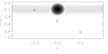
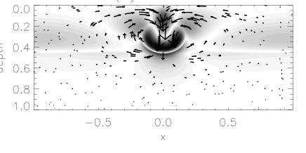
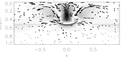
Figure 1: Velocity field superimposed on a grey scale representation of the entropy perturbation for a two-dimensional simulation of an entropy bubble oscillating in an isothermal atmosphere. The asterisks shown in panel (a) are used in Fig. 2a.

2.3 Numerics

The fully nonlinear set of equations (2) is solved using the hydrodynamical code described in Nordlund & Stein (1990) and Brandenburg et al. (1996). The time advance is explicit and uses a third order Hyman scheme (Hyman 1979). All spatial derivatives are calculated using sixth order compact finite differences (Lele 1992). The two-dimensional simulations presented here were done with the same resolution $256\times 300$ (i.e. 256 zones in the horizontal direction and 300 in the vertical) and aspect ratios, $A\equiv L_{z}/L_{x}$, between 2 and 6. Here, $L_{x}$ and $L_{z}$ denote the domain size in the horizontal and vertical directions, respectively. Moreover, the dimensionless sound speed and the gravitational acceleration are also the same for all runs and set equal to $c_{\rm s}=g=1$. As a consequence, the dimensionless pressure scale height is $H=3/5$ (i.e. the box extends over $1.66H$ in the vertical direction so that the density contrast between bottom and top is around $\rho_{\rm bot}/\rho_{\rm top}\simeq 5.3$), while the Brunt-Väisälä frequency is $N=\sqrt{2/3}\simeq 0.82$. Finally, the dimensionless kinematic viscosity $\nu$ has been set equal to $\nu=10^{-3}$ in all simulations, except in the study of the influence of the viscosity on the mode damping rates (Sect. 5.2) where we also considered smaller values down to $\nu=5\times 10^{-4}$.

As initial condition to excite IGWs in the layer, we choose the perturbation to be an entropy bubble (Brandenburg 1988). For a given entropy perturbation, it is indeed easy to find the approximate position of the point around which the bubble will begin to oscillate and thus generate IGWs. In dimensionless units we have

$$N^{2}=-\frac{ds^{\prime}}{dz}\simeq-\frac{\Delta s^{\prime}}{\Delta z},\quad\mbox{so}\quad\Delta z\simeq-\frac{\Delta s^{\prime}}{N^{2}}\simeq-\frac{3}{2}\Delta s^{\prime},$$

where $s^{\prime}\equiv s/c_{p}=(1/\gamma)\mathop{\hbox{ln}}\nolimits P-\mathop{\hbox{ln}}\nolimits\rho$ is the dimensionless entropy. All simulations start with an initial (negative) entropy perturbation $\Delta s^{\prime}=-0.2$ located at $z=0.2$ so that $\Delta z=0.3$. This cold bubble then falls down to the middle of the layer, $z=0.5$, and begins to oscillate around this point, generating IGWs. We note that the entropy perturbation is done at constant pressure $\Delta P=0$, i.e. $\Delta\ln\rho=-\Delta s^{\prime}$.

Figure 1 shows an example of such a two-dimensional hydrodynamical simulation where the velocity field has been superimposed onto a grey scale representation of the entropy. At $t=0$, the negative entropy perturbation looks like a bubble at $x=0$ and $z=0.2$ (Fig. 1a) and no velocity field is present. Under the effect of gravity, the bubble begins to descend (Fig. 1b) and stabilizes at the depth $z=0.5$. The bubble thus oscillates around this equilibrium position and IGWs are generated in the whole domain (Fig. 1c). The question is what is the spectrum and amplitude of the internal waves excited by this oscillating bubble.

3 Measuring IGWs excited by the oscillating bubble from classical methods

Two techniques are commonly used to measure wave fields propagating in direct hydrodynamical simulations:

Method 1 (hereafter M1):

the simplest method consists of firstly, recording the vertical velocity at a fixed point and, secondly, performing a Fourier transform of the time series. This method was used for example by Hurlburt et al. (1986) to detect IGWs in a simulation of penetrative convection.

Method 2 (hereafter M2):

a more precise method consists of, firstly, taking horizontal Fourier transforms of the vertical mass flux $\rho w$ for every time step and, secondly, computing power spectra for the individual time series. Peaks corresponding to acoustic or gravity oscillations thus appear at a given horizontal wavenumber $k_{x}$ in the $(z,\omega)$-plane. This method was used for example by Stein & Nordlund (1990) to determine the acoustic modes that are excited in their numerical simulations of solar granulation.

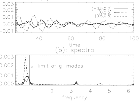
Figure 2: Detection of IGWs using method M1. (a): time evolution of the vertical velocity recorded at three different positions in the domain (denoted by stars in Fig. 1a). (b): corresponding temporal power spectra. Peaks below the buoyancy frequency $N=0.82$ correspond to internal gravity waves whereas the peak around $\omega=\pi$ is the fundamental acoustic mode.

In Fig. 2 we summarize the application of method M1 to detect the IGWs propagating in the simulation of Fig. 1. As expected for wave propagations, vertical velocities oscillate approximately periodically around zero at the three different levels (Fig. 2a). However, when we look at the corresponding temporal power spectra, only very few modes appear: the fundamental radial acoustic mode and one or two gravity modes below the bounding Brunt-Väisälä frequency $N\approx 0.82$ (Fig. 2b). We recall that gravity waves cannot propagate along the vertical direction so that the $g$-modes necessarily correspond to nonradial modes (e.g. Unno et al. 1989). Since method M1 does not take into account the horizontal dependence of the modes, nonradial $g$-modes with almost the same frequency but different horizontal wavenumber $k_{x}$ cannot be distinguished. This degeneracy in the mode degrees explains why only very few $g$-modes are captured with this method. Here and in the following we present the horizontal wavenumbers in terms of their smallest possible finite value, so that $k_{x}=(2\pi/L_{x})\ell$ where $\ell$ denotes the mode degree and is an integer, $\ell=[0,1,2,..]$.

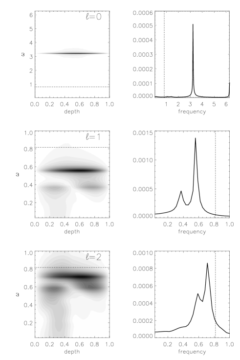
Figure 3: Detection of IGWs using method M2. Left: temporal power spectra in the $(z,\omega)$-plane for three different degrees $\ell=[0,1,2]$. Right: the resulting spectra after an integration in depth. Dotted lines shown in all plots correspond to the bounding frequency $\omega=N\approx 0.82$, above which $g$-modes cannot exist.

In Fig. 3 we summarize the application of the second method M2 to detect IGWs in the same simulation of Fig. 2. We now have access to more informations than with method M1. At first, the $\ell=0$ diagram confirms: (i) that the mode around $\omega=\pi$ is indeed a radial one and that it corresponds to the fundamental acoustic mode as no radial node is visible; (ii) that gravity modes are strictly nonradial modes as no peaks are visible below the dotted line $\omega=N$.

Second, gravity modes with similar frequency but different degrees $\ell$ are now well separated. As an example, the fundamental $g$-mode at $\ell=1$ and the first overtone at $\ell=2$ have almost the same frequency, $\omega\simeq 0.6$. Using the $(z,\omega)$-plane for different $\ell$’s allows us to separate modes and to show that one mode corresponds to a fundamental one while the other one is a first overtone [note the two “bumps” around $\omega\simeq 0.6$ in the $(z,\omega)$-diagram for $\ell=2$].

4 A new method using the anelastic subspace

The classical methods M1 and M2 presented above have some disadvantages which render them inappropriate for a careful detection of IGWs in hydrodynamical simulations:

• the main disadvantage of method M1 is its $k_{x}$-degeneracy, that is, the horizontal dependence of the modes is not taken into account. As a consequence, we have only access to a rough spectrum where only very few peaks appear.

• method M2 takes into account this horizontal dependence so that more modes are detected. But what about modes amplitudes? For example, this method does not permit to quantify the amount of kinetic energy due to IGWs propagating in the box so that only qualitative information, such as the knowledge of the spectrum of excited $g$-modes, is possible.

Finally, we recall that the goal of this work is to find a tool allowing us to measure quantitatively IGWs that are stochastically excited by penetrative convection. In view of this it is clear that methods M1 and M2 are not well adapted to this problem as Fourier transforms done to find the spectrum are calculated over the whole simulation.

Our new method, which eliminates these shortcomings, is inspired by the work of Bogdan, Cattaneo & Malagoli (1993, hereafter BCM) who have developed a tool to measure the acoustic emission generated in their simulations of turbulent convection. They extracted the acoustic field by projecting the convection field onto the acoustic subspace build from the eigenfunctions of the associated linear oscillations problem. Here we are interested in gravity waves rather than sound waves and this allows us to adopt a simpler procedure than theirs. Thus, we project our simulation data onto the anelastic subspace, that is, we filter out the acoustic waves in the linear system of oscillation equations. For a time dependence of normal modes of the form $\exp({\rm i}\omega t)$, and in the ideal limit $\nu=0$, the anelastic set of equations reduces to (Dintrans & Rieutord 2001; Rieutord & Dintrans 2002)

$$\left\{\begin{array}[]{l}\displaystyle\omega^{2}\@vec{\xi}=NewA\Pi+N^{2}\xi_{z}\@vec{e}_{z},\\ \\ \mathop{\hbox{div}}\nolimits(\rho_{0}\@vec{\xi})=0,\\ \\ \xi_{z}=0\quad\hbox{for}\quad z=0,1,\end{array}\right.$$ (3)

where $\@vec{\xi}=(\xi_{x},\xi_{z})$ denotes the Lagrangian displacement (the associated velocity field being $\@vec{v}={\rm i}\omega\@vec{\xi}$), $\Pi=P^{\prime}/\rho_{0}$ the eulerian perturbation in reduced pressure and $\rho_{0}(z)$ the equilibrium density profile.

Because we adopt periodic boundary conditions in the $x$-direction, we can seek solutions of the form

$$\xi_{x}(x,z)=\xi_{x}(z)\cos(k_{x}x)\quad\hbox{and}\quad\xi_{z}(x,z)=\xi_{z}(z)\sin(k_{x}x),$$

such that the anelastic system (3) reads after the elimination of $\Pi$

$$\left\{\begin{array}[]{l}\displaystyle\omega^{2}\left(\xi_{z}-\frac{1}{k_{x}}\frac{d\xi_{x}}{dz}\right)=N^{2}\xi_{z},\\ \\ \displaystyle-k_{x}\xi_{x}+\frac{d\xi_{z}}{dz}+\frac{d\mathop{\hbox{ln}}\nolimits\rho_{0}}{dz}\xi_{z}=0,\\ \\ \xi_{z}=0\quad\hbox{for}\quad z=0,1.\end{array}\right.$$ (4)

This last system can be formally rewritten as a generalized eigenvalue problem of the form

$${\cal M}_{A}\@vec{\psi}_{\ell n}=\omega^{2}_{\ell n}{\cal M}_{B}\@vec{\psi}_{\ell n},$$ (5)

where $\@vec{\psi}_{\ell n}=(\xi_{x},\xi_{z})^{T}$ is the eigenvector associated with eigenvalue $\omega^{2}_{\ell n}$ and ${\cal M}_{A}$, ${\cal M}_{B}$ denote two differential operators.

As shown in Appendix A, the eigenfunctions $\@vec{\psi}_{\ell n}$ which are solutions of the eigenvalue problem (5) are orthogonal, that is we have

$$\langle\@vec{\psi}_{\ell n},\@vec{\psi}_{\ell^{\prime}n^{\prime}}\rangle=\int_{0}^{1}\@vec{\psi}^{\dagger}_{\ell n}\cdot\@vec{\psi}_{\ell^{\prime}n^{\prime}}\rho_{0}{\rm d}z=\delta_{\ell\ell^{\prime}}\delta_{nn^{\prime}},$$ (6)

for normalized eigenfunctions (here the symbol $\dagger$ denotes the Hermitian conjugate). As a consequence, the set $\@vec{\psi}_{\ell n}$ forms an orthogonal basis onto which the simulated velocity field $\@vec{v}$ can be projected, i.e.

$$\@vec{v}(x,z,t)=\displaystyle\sum_{\ell=1}^{+\infty}\sum_{n=0}^{+\infty}\langle\@vec{\psi}_{\ell n},\@vec{v}\rangle\@vec{\psi}_{\ell n}(z)\left|\begin{array}[]{l}\cos(k_{x}x)\\ \\ \sin(k_{x}x)\end{array}\right.+\@vec{v}_{\hbox{\scriptsize rest}},$$ (7)

where the $\ell$-sum begins at $\ell=1$ as no gravity modes propagate radially, i.e. $k_{x}=(2\pi/L_{x})\ell$ should be non-zero (see Sect. 3). In this decomposition, the first term corresponds to the IGW contribution while all other rates, such as the bubble displacement or the acoustic waves, were collected in a term which we identify hereafter as “rest”. Finally, following BCM, we identify the amplitude of each gravity mode by the time-dependent coefficient

$$c_{\ell n}(t)=\langle\@vec{\psi}_{\ell n},\@vec{v}\rangle.$$ (8)

In the case of an isothermal atmosphere, for which $\rho_{0}$ and $N$ are simply given by (1), analytic expressions for both eigenvalues and eigenvectors of the anelastic system (4) can be found (see Appendix B) and we give here only the result:

$$\left\{\begin{array}[]{l}\displaystyle\omega_{\ell n}=N\left[1+\frac{1}{k_{x}^{2}}\left(\frac{1}{4H^{2}}+k^{2}_{z}\right)\right]^{-1/2},\\ \\ \displaystyle\xi^{\ell n}_{x}=\frac{C}{k_{x}}\exp(-z/2H)\left[k_{z}\cos(k_{z}z)+\frac{1}{2H}\sin(k_{z}z)\right],\\ \\ \xi^{\ell n}_{z}=C\exp(-z/2H)\sin(k_{z}z),\end{array}\right.$$ (9)

where we have introduced the vertical wavenumber $k_{z}=(n+1)\pi$. Because of these analytic expressions, the construction of the anelastic basis used in the projection (7) is straightforward. However, in practice, we do not project directly onto the two-dimensional velocity field but rather its horizontal Fourier transform at a given $k_{x}$, so that the procedure is the following:

1. given a $k_{x}$-value, we first deduce the anelastic eigenvalues $\omega_{\ell n}$ and eigenvectors $\psi_{\ell n}=(\xi^{\ell n}_{x},\xi^{\ell n}_{z})^{T}$ from their analytic expressions (9).

2. we build the anelastic subspace at this horizontal wavenumber $k_{x}$ with, say, the first five anelastic modes $n=[0,4]$.

3. we Fourier transform the simulated velocity field $\@vec{v}(x,z,t)$ to obtain the new complex-type field $\hat{\@vec{v}}_{\ell}(z,t)$.

4. we project $\hat{\@vec{v}}_{\ell}(z,t)$ onto the anelastic basis, built at step 2, and deduce the mode amplitudes (8) for each order $n$.

We will now illustrate the efficiency of our IGW detection method by measuring IGWs excited in the same simulation used to present methods M1 and M2 in Sect. 3.

5 Results

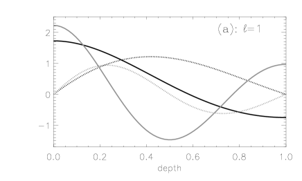
Figure 4: Vertical structure of the fundamental anelastic mode (dark line) and first overtone (grey line) at $\ell=1$ (a) and $\ell=2$ (b). Solid lines mark the horizontal displacement $\xi_{x}$ while dot-dashed lines are for the vertical one $\xi_{z}$. Eigenfunctions have been normalized by imposing $\int_{0}^{1}|\psi_{\ell n}|^{2}\rho_{0}dz=1$.

5.1 The anelastic eigenvectors: comparisons with the simulation profiles

Figure 4 shows four anelastic modes at $\ell=1$ (a) and $\ell=2$ (b) with $n=0$ (dark lines) and $n=1$ (grey lines). We remark that anelastic eigenfunctions hardly change with the $\ell$-values as $\xi_{z}$ does not explicitly depend on $k_{x}$, while only the $\xi_{x}$-amplitude involves $k_{x}$. As a consequence, it is the ratio $\xi_{z}/\xi_{x}\propto k_{x}$ which makes sense so that $\xi_{z}$ becomes more and more important compared to $\xi_{x}$ with increasing $k_{x}$, as observed in Fig. 4 when comparing solid to dot-dashed lines for the same order $n$. In the case of method M2, the use of the vertical mass flux $\rho_{0}v_{z}$ (instead of, say, $\rho_{0}v_{x}$) is justified a posteriori as a good proxy for detecting IGWs propagating in the simulation (see Fig. 3).

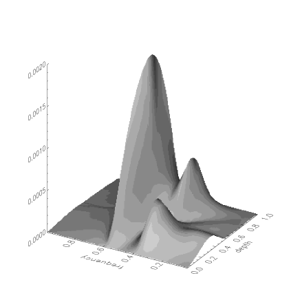
Figure 5: Upper: same as Fig. 3 at $\ell=1$, except that amplitudes have been restored using third direction. Lower: comparisons between the normalized vertical mass flux $\rho_{0}v_{z}$ profiles deduced from the upper power spectra (solid lines) with the ones obtained from the anelastic modes shown in Fig. 4a (dotted lines).

Once the anelastic eigenfunctions are known, one can compare the corresponding vertical mass flux $\rho_{0}v_{z}$ with the ones deduced from the power spectra used in method M2. Indeed, the peaks appearing at a given frequency in Fig. 3 correspond to $g$-modes so that their vertical profiles can be related to the eigenfunctions of the linear modes. This was done by BCM for the case of acoustic modes propagating in their convection simulations.

The upper panel of Fig. 5 shows the depth dependence of the two peaks appearing at $\ell=1$ in Fig. 3, which correspond to the $n=0$ ($\omega_{10}=0.568$) and $n=1$ ($\omega_{11}=0.363$) modes, respectively. We thus recover what BCM called the “shark fin” profiles, that is, the power at any depth is located around the theoretical anelastic frequency. Taking a mean profile around eigenfrequencies $\omega_{10}$ and $\omega_{11}$ allows us to compare the vertical mass flux observed in the simulation with those calculated from the linear anelastic modes. The lower panel of Fig. 5 shows that the agreement between the two profiles is quite remarkable, meaning that the anelastic modes reproduce well the long-period dynamics of the oscillating isothermal atmosphere.

5.2 Time evolution of the mode amplitudes $c_{\ell n}(t)$

Figure 6: Left: real parts of the complex mode amplitude $c_{\ell n}(t)$ for the three modes shown in Fig. 4. Right: corresponding temporal power spectra. Dotted lines mark the location of the anelastic eigenmodes $\omega_{10}=0.568,\ \omega_{11}=0.363$ and $\omega_{21}=0.575$, respectively. Amplitudes on each plot have been multiplied by one thousand.

The left hand panel of Fig. 6 shows the real parts of the complex amplitudes $c_{10},\ c_{11}$ and $c_{21}$, that is, the result of the projection of the simulation shown in Fig. 1 onto the three anelastic modes plotted in Fig. 4. By taking a Fourier transform of these sequences (Fig. 6, right), one obtains three peaks which agree remarkably well with the theoretical anelastic frequency given by (9), i.e. the complex amplitudes $c_{\ell n}$ behave as

$$c_{\ell n}\propto\exp({\rm i}\omega_{\ell n}t).$$ (10)

This relation means that when an eigenmode is excited in the simulation, its corresponding displacement is periodic with a period $T_{\ell n}=2\pi/\omega_{\ell n}$.

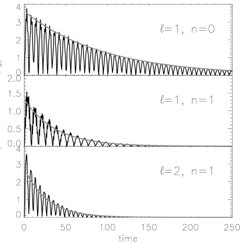
Figure 7: Time-evolution of the amplitude modulus $|c_{\ell n}|$ for the three modes shown in Fig. 4. Grey lines superimposed correspond to an exponential decay of the form $|c_{\ell n}|\propto\exp(-\alpha t)$.

As we have access to the real and imaginary parts of $c_{\ell n}$, we now compute the amplitude modulus $|c_{\ell n}|$; Fig. 7 shows its time evolution for the three modes in Fig. 6. A regression analysis of the curves $\max(|c_{\ell n}|)=f(t)$ allows us to determine the shape of the envelope and we found that $|c_{\ell n}|$ follows a simple exponential decay law of the form $\exp(-\alpha t)$. Because of the periodic behaviour (10), it means that the mode amplitude behaves like

$$c_{\ell n}\propto\exp(-\alpha t)\exp({\rm i}\,\omega_{\ell n}t),$$ (11)

where $\alpha$ is a constant which is related to the damping process, here the viscosity. Using runs with different kinematic viscosities we have verified that $\alpha\propto\nu$, i.e. every mode obeys the same law as that of a linear damped harmonic oscillator. Such a relation between the damping of the mode and the viscosity is hardly surprising as it can easily be deduced from work integrals; see Appendix C.

5.3 Contributions of $g$-modes to the time-averaged kinetic energy

Figure 8: Dependence of the time-averaged kinetic energy on degree $\ell$ and radial order $n$.

We will now show that one of the main advantages of the anelastic subspace resides in the fact that it allows to calculate the contribution of every $g$-mode to the time-averaged kinetic energy. We demonstrate in Appendix D that a Parseval-Bessel relation also exists in the anelastic subspace as

$$\int_{V}\rho_{0}\@vec{v}^{2}(x,z)\,{\rm d}x\,{\rm d}z=\sum^{+\infty}_{\ell,n}|c_{\ell n}|^{2}+{\rm rest},$$ (12)

where, as before, the rest term contains all the contributions which are not due to IGWs.

This relation illustrates the usefulness of the anelastic subspace when one wants to perform a detailed study of the IGW excitation. By using the classical Parseval-Bessel relation applied in Fourier space, it is already possible to find the amount of kinetic energy contained at a given wavenumber $k_{x}$, since

$$\int_{V}\rho_{0}\@vec{v}^{2}(x,z)\,{\rm d}x\,{\rm d}z=\int_{z}\sum^{+\infty}_{\ell}|\hat{\@vec{v}}_{\ell}|^{2}\rho_{0}\,{\rm d}z.$$ (13)

For example, the dependence of the time-averaged kinetic energy on the degree $\ell$, shown in Fig. 8, demonstrates that half of the kinetic energy in the simulation in Fig. 1 is contained in the $\ell=1$ degree (the solid line denoted by “$g$-modes + rest”). Unfortunately, this curve gives no information about the vertical dependence of this distribution so that contributions coming from nonradial acoustic modes as well as gravity modes can be present.

The main advantage of our anelastic subspace method is that it lifts this degeneracy by isolating contributions that come from $g$-modes only. Comparing to its classical form (13), the anelastic Parseval-Bessel relation (12) introduces the radial order $n$ so that one can extract the contribution of the $g$-mode $(\ell,n)$ in the kinetic energy and then deduce which modes contribute most to it, meaning the modes that are the most excited by the oscillating bubble. This is what we did in Fig. 8 where we also plotted, for each $\ell$, the contributions coming from the $n=0$, $n=1$ and $n=2$ $g$-modes. It allows us to show that the $\ell=1$ contribution is in fact almost entirely composed of the $(1,0)$ and $(1,1)$ $g$-modes, as they respectively contain around 33% and 15% of the time-averaged kinetic energy of this simulation. This kind of information is particularly relevant when one deals with the problem of wave excitation.

5.4 Effects of the box geometry on modes amplitudes

In order to assess the restriction imposed by the finite size of the box, we now study the influence of the box geometry onto the wave excitation. We therefore perform three runs with three different aspect ratios (2, 4 and 6) and calculate the $g$-mode contributions to the time-averaged kinetic energy in each case.

Figure 9 shows the spectral power in the $(k_{x},\omega)$ plane for the three different aspect ratios. One recovers clearly the well-known dispersion relation for $g$-modes (e.g. Stein & Leibacher 1974); see also its anelastic counterpart in Eq. (9). One also verifies that increasing the horizontal extent of the box allows the power to be distributed among a larger number of horizontal modes. This phenomenon has also been observed in the problem of $p$-modes excitation by turbulent convection (Stein & Nordlund 2001; Nordlund & Stein 2001). Unfortunately, such diagrams are generally not easy to interpret when the system is not isothermal and the modes stochastically driven; see for example the three-dimensional simulations of Brandenburg et al. (1996) where the resulting $(k_{x},\omega)$ turned out to be very noisy.

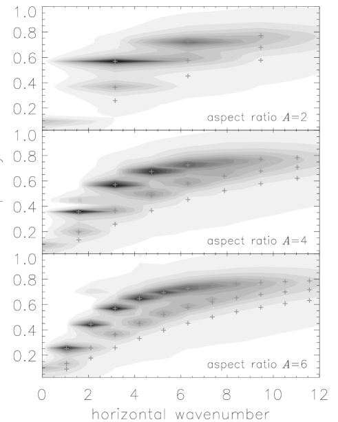
Figure 9: $(k_{x}-\omega)$ diagrams which three different aspect ratios (2, 4 and 6). Crosses correspond to the anelastic frequencies given by (9).

Figure 10: Distribution of the energy contained in $g$-modes for different aspect ratios (2,4 and 6) in a log-log representation.

Contrasting this with the anelastic subspace method, it is straightforward to extract at a given wavenumber $k_{x}$ the energy from modes with different radial order $n$. As expected, the spectral distribution of mode energies integrated over all $n$ collapses onto an universal curve (Fig. 10). It turns out that the mode energy scales as $\sim k_{x}^{-2/3}$ for small enough values of $k_{x}$, i.e. for $k_{x}L_{x}/A\raisebox{-3.01385pt}{$\stackrel{{\scriptstyle<}}{{\sim}}$}10$. However, both the exponent and the cut-off are not unique and depend on the size of the initial entropy bubble, as verified by running several simulations with bubble radii ranging from $R=0.1$ to $R=0.4$. We found that the larger the bubble, the smaller is the cutoff value of $k_{x}$, meaning that big bubbles preferentially generate $g$-modes at large scales. It would be interesting to investigate in more detail the origin of such behaviour, but this is clearly beyond the scope of this paper.

6 Conclusions

We have presented a new and accurate method to measure the internal gravity waves propagating in a numerical simulation. This is of prime importance when one deals with the problem of the generation of IGWs in a stably stratified medium such as the radiative zone of a star. The knowledge of the vigour of the velocity field in such a zone is the main input of any theory of wave transport of angular momentum and/or chemicals in stellar radiative zones (e.g. Schatzman 1993).

However, we have shown that classical methods based only on Fourier transforms in space and/or time of the simulated velocity field do not allow a quantitative determination of the mode amplitudes. The reason is mainly that the contribution of the propagating $g$-modes to the total energy in the simulation is diluted among the other ones due to $p$-modes and turbulent motions.

Our method is based on the projection of the simulated velocity field onto the anelastic subspace built from the solutions of the linear problem for the perturbations. Once the resulting time-dependent coefficients of the velocity field are computed, one can deduce the amplitudes of every $g$-mode and measure their kinetic energy at every timestep of the simulation.

We have applied this formalism to the measurement of IGWs excited by an entropy bubble oscillating in an isothermal atmosphere. We have shown that the mode amplitudes follow the same law than those of a linear damped harmonic oscillator, that is, the periodic amplitudes decrease exponentially with time, with a time scale that is simply proportional to the inverse of the viscosity; see Eq. (11). By using a Parseval-Bessel relation valid in the anelastic subspace, we have deduced the contribution of every $g$-mode to the time-averaged kinetic energy and have shown that large-scale motions are mainly composed of $n=0$ and $n=1$ modes. Such a result is in general impossible to obtain in a more complicated settings using a classical $(k_{x}-\omega)$ diagram.

The fact that the mode amplitudes in the anelastic basis follow the same law than those of a linear damped oscillator is important in the case of a stochastic excitation of IGWs, such as the one encountered when one deals with numerical simulations of penetrative convection. Indeed, in this case the mode amplitude $c_{\ell n}$ evolves either chaotically around zero when the mode is not excited, or in a periodic fashion following Eq. (11) when the mode is excited. By computing time-frequency diagrams of that time-dependent amplitude, one can extract the time intervals during which the mode has been really excited. In a forthcoming paper, we will present the application of the anelastic subspace method we tested here to the problem of IGWs stochastically excited by penetrative convection (Dintrans et al. 2004).

Appendix A Orthogonality of the anelastic eigenfunctions

We start from the complete set of equations written for two eigenmodes $(\omega_{1},\@vec{\xi}_{1})$ and $(\omega_{2},\@vec{\xi}_{2})$ (Dintrans & Rieutord 2001)

$$\left\{\begin{array}[]{l}\omega_{1}^{2}\rho_{0}\@vec{\xi}_{1}=\rho_{0}NewA\Pi_{1}+N^{2}\rho_{0}\xi^{(1)}_{z}\@vec{e}_{z},\\ \\ \omega_{2}^{2}\rho_{0}\@vec{\xi}_{2}=\rho_{0}NewA\Pi_{2}+N^{2}\rho_{0}\xi^{(2)}_{z}\@vec{e}_{z},\\ \\ \mathop{\hbox{div}}\nolimits(\rho_{0}\@vec{\xi}_{1})=\mathop{\hbox{div}}\nolimits(\rho_{0}\@vec{\xi}_{2})=0,\\ \\ \xi^{(1)}_{z}=\xi^{(2)}_{z}=0\quad\hbox{for}\quad z=0,1,\par\end{array}\right.$$ (14)

where $\Pi=P^{\prime}/\rho_{0}$ denotes the eulerian fluctuation of the reduced pressure. Multiplying the $\@vec{\xi}_{1}$-equation by $\@vec{\xi}_{2}$ and the $\@vec{\xi}_{2}$-equation by $\@vec{\xi}_{1}$, and subtracting the resulting two equations leads to

$$(\omega_{1}^{2}-\omega_{2}^{2})\rho_{0}\@vec{\xi}_{1}\cdot\@vec{\xi}_{2}=\mathop{\hbox{div}}\nolimits(\Pi_{1}\rho_{0}\@vec{\xi}_{2})-\mathop{\hbox{div}}\nolimits(\Pi_{2}\rho_{0}\@vec{\xi}_{1}),$$ (15)

where we have used the relation $\rho_{0}\@vec{\xi}_{2}\cdot NewA\Pi_{1}=\mathop{\hbox{div}}\nolimits(\Pi_{1}\rho_{0}\@vec{\xi}_{2})-\Pi_{1}\mathop{\hbox{div}}\nolimits(\rho_{0}\@vec{\xi}_{2})=\mathop{\hbox{div}}\nolimits(\Pi_{1}\rho_{0}\@vec{\xi}_{2})$, as the anelastic approximation implies $\mathop{\hbox{div}}\nolimits(\rho_{0}\@vec{\xi}_{2})=0$.

Finally, we integrate this last equation over the volume and use the Green-Ostrogradsky theorem to obtain

$$(\omega_{1}^{2}-\omega_{2}^{2})\int_{V}\rho_{0}\@vec{\xi}_{1}\cdot\@vec{\xi}_{2}{\rm d}V=\int_{S}\Pi_{1}\rho_{0}\@vec{\xi}_{2}\cdot{\rm d}\@vec{S}-\int_{S}\Pi_{2}\rho_{0}\@vec{\xi}_{1}\cdot{\rm d}\@vec{S}.$$ (16)

The applying of periodic horizontal boundary conditions and the condition $\xi_{z}=0$ at $z=0$ and $z=1$ leads to the vanishing of the two right hand side terms. The uniqueness of the solutions ensures that $\omega_{1}\neq\omega_{2}$ so that we conclude that the eigenvectors are orthogonal to each other, i.e.

$$\int_{V}\rho_{0}\@vec{\xi}_{1}\cdot\@vec{\xi}_{2}{\rm d}V=0.$$ (17)

Appendix B Anelastic oscillations of an isothermal atmosphere

B.1 Derivation of the anelastic eigenfrequencies and eigenfunctions

We start from the anelastic set of equations (4)

$$\left\{\begin{array}[]{l}\displaystyle\frac{N^{2}}{\omega^{2}}\xi_{z}=\xi_{z}-\frac{1}{k_{x}}\frac{d\xi_{x}}{dz},\\ \\ \displaystyle-k_{x}\xi_{x}+\frac{d\xi_{z}}{dz}+\frac{d\mathop{\hbox{ln}}\nolimits\rho_{0}}{dz}\xi_{z}=0,\\ \\ \xi_{z}=0\quad\hbox{for}\quad z=0,1,\end{array}\right.$$ (18)

where, for an isothermal atmosphere, $\rho_{0}(z)$ and $N^{2}$ are given by Eq. (1). By eliminating $\xi_{x}$, we arrive at the following second-order differential equation for $\xi_{z}$

$$\left\{\begin{array}[]{l}\displaystyle\frac{d^{2}\xi_{z}}{dz^{2}}+\frac{1}{H}\frac{d\xi_{z}}{dz}-k_{x}^{2}\left(1-\frac{N^{2}}{\omega^{2}}\right)\xi_{z}=0,\\ \\ \xi_{z}(0)=\xi_{z}(1)=0.\end{array}\right.$$ (19)

All coefficients of this differential equation being constants, we can seek solutions of exponential type $\xi_{z}\propto\exp(rz)$ to obtain the characteristic equation

$$r^{2}+\frac{r}{H}-k_{x}^{2}\left(1-\frac{N^{2}}{\omega^{2}}\right)=0,$$ (20)

whose general solution is of the form

$$r=\frac{1}{2}\left(-\frac{1}{H}\pm{\rm i}\sqrt{\Delta}\right)\quad\hbox{with}\quad\Delta=-\frac{1}{H^{2}}-4k_{x}^{2}\left(1-\frac{N^{2}}{\omega^{2}}\right),$$ (21)

leading to the following solution for $\xi_{z}$

$$\xi_{z}(z)=\exp(-z/2H)\left[A\cos\left(\frac{\sqrt{\Delta}}{2}z\right)+B\sin\left(\frac{\sqrt{\Delta}}{2}z\right)\right].$$ (22)

To find the quantization rule for $\Delta$, we consider the boundary conditions on $\xi_{z}$,

$$\left\{\begin{array}[]{l}\xi_{z}(0)=0\Rightarrow A=0,\\ \\ \displaystyle\xi_{z}(1)=0\Rightarrow\frac{\sqrt{\Delta_{n}}}{2}=(n+1)\pi\quad\hbox{or}\quad\Delta_{n}=4(n+1)^{2}\pi^{2},\end{array}\right.$$ (23)

where $n=[0,1,2\dots]$ is the radial order of the mode. [The presence of the $n+1$ factor in the quantization rule is consistent with the fact that $\Delta$ is strictly non-zero.] We recall that the definition (21) for $\Delta$ allows us to deduce an expression for the anelastic eigenfrequencies,

$$\omega_{\ell n}=N\left[1+\frac{1}{k_{x}^{2}}\left(\frac{1}{4H^{2}}+k_{z}^{2}\right)\right]^{-1/2}\mbox{with $k_{z}=(n+1)\pi$},$$ (24)

and their associated eigenfunctions

$$\left\{\begin{array}[]{l}\displaystyle\xi^{\ell n}_{x}=\frac{C}{k_{x}}\exp(-z/2H)\left[k_{z}\cos(k_{z}z)+\frac{1}{2H}\sin(k_{z}z)\right],\\ \\ \xi^{\ell n}_{z}=C\exp(-z/2H)\sin(k_{z}z).\end{array}\right.$$ (25)

The remarkable fact to be noted here is that the vertical lagrangian displacement $\xi^{\ell n}_{z}$ does not depend on $k_{x}$ (the horizontal wavenumber) but only on the mode order $n$ (see Fig. 4).

B.2 Comparisons with the complete case

Table 1: Exact eigenfrequencies $\omega$ for the first five $g$-modes of degree $\ell=1$, corresponding to an horizontal wavenumber $k_{x}=2\pi/L_{x}=\pi$ (here $L_{x}=2$), in the complete case, in the anelastic approximation, and the corresponding relative errors.

Order $n$	$\omega$	$\omega_{\hbox{\scriptsize anel}}$	rel. error
0	0.572 054	0.567 455	0.804%
1	0.363 084	0.362 606	0.132%
2	0.257 381	0.257 295	0.033%
3	0.197 644	0.197 621	0.012%
4	0.159 920	0.159 912	0.005%

The set of equations for the complete case is obtained by, first, linearizing the system (2) for infinitesimal adiabatic perturbations and, second, by assuming the time and horizontal dependences of the modes to be $\exp({\rm i}\omega t)$ and $\cos(k_{x}x)$ or $\sin(k_{x}x)$, respectively. We thus arrive at

$$\left\{\begin{array}[]{l}\omega^{2}\xi_{x}=k_{x}\Pi,\\ \\ \displaystyle\omega^{2}\xi_{z}=\frac{d\Pi}{dz}+N^{2}\left(\xi_{z}+\frac{\Pi}{g}\right),\\ \\ \displaystyle\Pi=-c^{2}_{s}\left(-k_{x}\xi_{x}+\frac{d\xi_{z}}{dz}\right)-g\xi_{z},\\ \\ \displaystyle\xi_{z}=0\quad\hbox{for}\quad z=0,1.\end{array}\right.$$ (26)

Here $\Pi=P^{\prime}/\rho_{0}$ and $\rho^{\prime}$ are the eulerian perturbations in reduced pressure and density, respectively. This system has been obtained under the classical Cowling approximation which assumes that perturbations in the gravitational potential are negligible (Cowling 1941). We refer the reader to the book of Unno et al. (1989) for a complete derivation of this system in the case of a spherical geometry.

Figure 11: Comparison of the complete (solid lines) and anelastic (dashed lines) normalized eigenfunctions $\xi_{x}$ for $\ell=1$ and $n=[0,1,2]$.

Lamb (1909, 1932) found analytical solutions of the system (26) in the case of an isothermal atmosphere. By eliminating $\xi_{x}$ and $\Pi$ in the system (26), we obtain a second-order differential equation for $\xi_{z}$ only,

$$\left\{\begin{array}[]{l}\displaystyle\frac{d^{2}\xi_{z}}{dz^{2}}+\frac{1}{H}\frac{d\xi_{z}}{dz}+\left[\frac{\omega^{2}}{c^{2}_{s}}-k_{x}^{2}\left(1-\frac{N^{2}}{\omega^{2}}\right)\right]\xi_{z}=0,\\ \\ \xi_{z}(0)=\xi_{z}(1)=0.\end{array}\right.$$ (27)

Comparison with Eq. (19) shows that the anelastic approximation applies provided that:

• the Lamb frequency term $\omega^{2}/c^{2}_{s}$ is negligible, implying that

  $$\frac{\omega}{N}\ll k_{x}\frac{c_{\rm s}}{\omega},$$ (28)

  which is a condition naturally fulfilled by high-order $g$-modes with $\omega\ll N$.

• the ratio $k_{x}c_{\rm s}/N$ is very large

The solutions of the complete system (27) can be deduced from the anelastic ones as only the $\Delta$-term is changing, that is,

$$\Delta_{\hbox{\scriptsize compl}}=-\frac{1}{H^{2}}+4\left[\frac{\omega^{2}}{c^{2}_{s}}-k_{x}^{2}\left(1-\frac{N^{2}}{\omega^{2}}\right)\right],$$ (29)

while the same quantization rule applies due to the identical boundary conditions $\xi_{z}(0)=\xi_{z}(1)=0$, that is,

$$\Delta_{\hbox{\scriptsize compl}}=4(n+1)^{2}\pi^{2}=4k_{z}^{2}.$$ (30)

We thus obtain the following quadratic dispersion relation for the complete eigenfrequencies

$$\omega^{4}-c^{2}_{s}\left(k_{x}^{2}+k_{z}^{2}+\frac{1}{4H^{2}}\right)\omega^{2}+k_{x}^{2}c^{2}_{s}N^{2}=0,$$ (31)

which is the same than that in Stein & Leibacher (1974). In the same way, the eigenvectors of the complete case can be deduced from the anelastic ones and we find

$$\left\{\begin{array}[]{l}\displaystyle\xi^{\ell n}_{x}=\frac{C}{k_{x}}\exp(-z/2H)\left[k_{z}\cos(k_{z}z)+\frac{1}{H}\left(\frac{1}{\gamma}-\frac{1}{2}\right)\sin(k_{z}z)\right],\\ \\ \xi^{\ell n}_{z}=C\exp(-z/2H)\sin(k_{z}z).\end{array}\right.$$

Despite its different $\Delta$-term (29), we note that in the complete case the vertical displacement $\xi_{z}$ is the same as in the anelastic one, which is simply a consequence of applying the same quantization rule (30).

We summarize in Table (1) the eigenfrequencies for the complete case deduced from (31) for the first five $g$-modes of degree $\ell=1$ and compare them with their anelastic counterparts given by the formulæ (24). The agreement is quite remarkable since the relative error done by the anelastic approximation is less than $1\%$ from the fundamental $g$-mode. Concerning the associated eigenvectors, we showed that the vertical displacements $\xi_{z}$ are the same in both cases so that only the horizontal ones differ. However, Figure 11 shows that the agreement on the normalized $\xi_{x}$-eigenfunctions is also very good, except for the mode at $n=0$ for which the condition (28) is not well fulfilled.

In conclusion, the filtering of acoustic waves from the dynamics of the isothermal atmosphere does almost not change the $g$-mode eigenfrequencies $\omega_{\ell n}$ and eigenfunctions $\psi_{\ell n}=(\xi_{x},\xi_{z})^{T}$. The basis built from these anelastic eigenfunctions can therefore be used with good confidence to project out velocity fields from hydrodynamical simulations.

It should be pointed out that the application of the anelastic subspace method will only give good results when the acoustic and gravity spectra are well separated, that is, when the ratio $k_{x}c_{s}/N$ is large. This is the case for the chosen isothermal setup, where the resulting anelastic eigenfrequencies/eigenvectors are very close to those of the complete problem (see Table 1 and Fig. 11). However, this ratio decreases with larger stratification, in which case one may be forced to solve numerically the oscillation equations (26) of the complete problem instead of those of the anelastic subset (18), which does not however introduce any particular difficulty.

Appendix C Damping rate of the modes using work integrals

We show in this appendix that it is possible to find the relation governing the damping rate of a mode and the viscosity using the work integrals formalism. We start from the anelastic equations written for the velocity

$$\left\{\begin{array}[]{l}\lambda\@vec{u}=-NewA\Pi-N^{2}\xi_{z}\@vec{e}_{z}+\nu\Delta\@vec{u},\\ \\ \mathop{\hbox{div}}\nolimits(\rho_{0}\@vec{u})=0,\\ \\ u_{z}=0\quad\hbox{for}\quad z=0,1,\end{array}\right.$$ (32)

where $\lambda=\alpha+i\omega$ has a non-zero real part due to the viscous dissipation. We note that the viscous term is normally more complicated as there may be a vertical variation of the dynamical viscosity $\mu=\rho\nu$ [see the general form of this term in Eq. (2)]. However, we take here a simpler form as our aim is just to formally prove that the damping rate $\alpha$ is linearly related to the viscosity $\nu$.

We multiply the momentum equation by $\rho_{0}\@vec{u}^{*}$ to obtain

$$\lambda\rho_{0}\@vec{u}^{2}=-NewA(\rho\Pi\@vec{u}^{*})-N^{2}\rho_{0}\xi_{z}u^{*}_{z}+\nu\rho_{0}\@vec{u}^{*}\cdot\Delta\@vec{u},$$ (33)

where we have used $\mathop{\hbox{div}}\nolimits(\rho_{0}\@vec{u}^{*})=0$. As in Appendix A, we finally integrate this last equation over the volume and use the Green-Ostrogradsky theorem to obtain

$$\lambda\int_{V}\left(\rho_{0}\@vec{u}^{2}+N^{2}\rho_{0}\xi^{2}_{z}\right){\rm d}V=\nu\int_{V}\rho_{0}\@vec{u}^{*}\cdot\Delta\@vec{u}{\rm d}V,$$ (34)

where we also used $u^{*}_{z}=\lambda\xi^{*}_{z}$. As we only have real integrals on both sides, we can deduce the following relation for the real part $\alpha$

$$\alpha=\nu\frac{\int_{V}\rho_{0}\@vec{u}^{*}\cdot\Delta\@vec{u}{\rm d}V}{\int_{V}\left(\rho_{0}\@vec{u}^{2}+N^{2}\rho_{0}\xi^{2}_{z}\right){\rm d}V}.$$ (35)

The damping rate of a mode is therefore linearly related to the viscosity, as found numerically in (11).

A similar relation also applies in the complete case, provided one includes the contribution of pressure fluctuations to the energy, that is,

$$\alpha=\nu\frac{\int_{V}\rho_{0}\@vec{u}^{*}\cdot\Delta\@vec{u}{\rm d}V}{\int_{V}\left(\rho_{0}\@vec{u}^{2}+N^{2}\rho_{0}\xi^{2}_{z}+\frac{\Pi}{c^{2}_{s}}\right){\rm d}V}\equiv\frac{\hbox{viscous dissipation}}{\hbox{total energy}},$$

where the total energy contains the kinetic ($\rho_{0}u^{2}$), potential ($N^{2}\rho_{0}\xi^{2}_{z}$) and internal ($\rho_{0}\Pi/c^{2}_{s}$) contributions. Such relations are useful from a numerical point of view as they allow to check the accuracy of the computed eigenvalues from their associated eigenvectors.

Appendix D Parseval-Bessel relation in the anelastic subspace

In this appendix, we will show that it is possible to relate the total kinetic energy embedded in the box to the one calculated in the anelastic subspace. To do that, we need a similar relation than the Parseval-Bessel one which states that the total energy is conserved when one works in Fourier space, i.e.

$$\int_{V}f^{2}(x,y,z)\,{\rm d}V=\int_{k}|\hat{f}|^{2}{\rm d}^{3}k,$$ (36)

where $\hat{f}$ denotes the Fourier transform of $f$.

In our case, we only perform a 1-D Fourier transform of the velocity field in the horizontal direction (corresponding to a wavenumber $k_{x}=(2\pi/L_{x})\ell$), so that the Parseval-Bessel relation for the total kinetic energy at a given time is

$$\int_{V}\rho_{0}\@vec{v}^{2}(x,z)\,{\rm d}x\,{\rm d}z=\int_{z}\sum^{+\infty}_{\ell}|\hat{\@vec{v}}_{\ell}|^{2}\rho_{0}\,{\rm d}z,$$ (37)

where $\hat{\@vec{v}}_{\ell}$ denotes the velocity field at a wavenumber $k_{x}$. We now introduce the anelastic subspace by using the relation which links the velocity field in Fourier space to the one in the anelastic space as

$$\hat{\@vec{v}}_{\ell}(z)=\sum^{+\infty}_{n}\langle\@vec{\psi}_{\ell n},\hat{\@vec{v}}_{\ell}\rangle\@vec{\psi}_{\ell n}(z)+{\rm rest}.$$ (38)

The $z$-integral in Eq. (37) can then be calculated in the anelastic subspace as

$$\begin{array}[]{ll}\displaystyle\int_{z}|\hat{\@vec{v}}_{\ell}|^{2}\rho_{0}\,{\rm d}z=\int_{z}\hat{\@vec{v}}^{\dagger}_{\ell}\hat{\@vec{v}}_{\ell}\rho_{0}\,{\rm dz},\\ \\ \displaystyle\hskip 14.22636pt=\sum^{+\infty}_{n}\langle\@vec{\psi}_{\ell n},\hat{\@vec{v}}_{\ell}\rangle\int_{z}\hat{\@vec{v}}^{\dagger}_{\ell}\@vec{\psi}_{\ell n}(z)\rho_{0}\,{\rm d}z+{\rm rest},\\ \\ \displaystyle\hskip 14.22636pt=\sum^{+\infty}_{n}\langle\@vec{\psi}_{\ell n},\hat{\@vec{v}}_{\ell}\rangle\langle\hat{\@vec{v}}_{\ell},\@vec{\psi}_{\ell n}\rangle+{\rm rest},\\ \\ \displaystyle\hskip 14.22636pt=\sum^{+\infty}_{n}|c_{\ell n}|^{2}+{\rm rest}.\end{array}$$ (39)

This last equation means that the total kinetic energy due to $g$-modes at a given $k_{x}$ and time $t$ is simply given by the sum over the radial orders $n$ of the squares of the mode amplitudes. By taking into account the $k$-integral, we finally obtain the Parseval-Bessel relation written in the anelastic subspace as

$$\int_{V}\rho_{0}\@vec{v}^{2}(x,z)\,{\rm d}x\,{\rm d}z=\sum^{+\infty}_{\ell,n}|c_{\ell n}|^{2}+{\rm rest}.$$ (40)

References

- (1) Bogdan, T. J., Cattaneo, F., & Malagoli, A. 1993, ApJ, 407, 316
- (2) Brandenburg, A. 1988, A&A, 203, 154
- (3) Brandenburg, A., Jennings, R. L., Nordlund, Å., Rieutord, M., Stein, R. F., & Tuominen, I. 1996, J. Fluid Mech., 306, 325
- (4) Brummell, N. H., Clune, T. L., & Toomre, J. 2002, ApJ, 570, 825
- (5) Cowling, T. G. 1941, MNRAS, 101, 367
- (6) Dintrans, B., Brandenburg, A., Nordlund, Å., & Stein, R. F. 2003, Ap&SS, 284, 237
- (7) Dintrans, B., Brandenburg, A., Nordlund, Å., & Stein, R. F. 2004, in preparation.
- (8) Dintrans, B. & Rieutord, M. 2001, A&A, 324, 635
- (9) Gabriel, A. H., Baudin, F., Boumier, P., García, R. A., Turck-Chièze, S., Appourchaux, T., Bertello, L., Berthomieu, G., Charra, J., Gough, D. O., Pallé, P. L., Provost, J., Renaud, C., Robillot, J.-M., Roca Cortés, T., Thiery, S., & Ulrich, R. K. 2002, A&A, 390, 1119
- (10) Hurlburt, N. E., Toomre, J., & Massaguer, J. M. 1986, ApJ, 311, 563
- (11) Hurlburt, N. E., Toomre, J., Massaguer, J. M., & Zahn, J. P. 1994, ApJ, 241, 245
- (12) Hyman, J. M. 1979, In: Adv. in Computation Methods for Partial Differential Equations, Vol. III, Eds: R. Vichnevetsky & R. S. Stepleman, Publ. IMACS, p. 313
- (13) Kumar, P., Talon, S., & Zahn, J.-P. 1999, ApJ, 520, 859
- (14) Lamb, H. 1909, Proc. Lond. Math. Soc. (2), 7, 122
- (15) Lamb, H. 1932, Hydrodynamics (Dover Publications)
- (16) Lele, S. K. 1992, J. Comp. Phys., 103, 16
- (17) Nordlund, Å., & Stein, R. F. 1990, Comput. Phys. Commun., 59, 119
- (18) Nordlund, Å., & Stein, R. F. 2001, ApJ, 546, 576
- (19) Press, W. H., Teukolsky, S. A., Vetterling, W. T., & Flannery, B. P. 1994, Numerical Recipes in Fortran. The Art of Scientific Computing. 2nd Edition (Cambridge University Press)
- (20) Rieutord, M. & Dintrans, B. 2002, MNRAS, 337, 1087
- (21) Stein, R. F. & Leibacher, J. 1974, A&AR, 12, 407
- (22) Stein, R. F. & Nordlund, Å. 1990, Progress in Seismology of the Sun and Stars. Lecture Notes in Physics, Springer-Verlag, Berlin, 367, 93
- (23) Stein, R. F. & Nordlund, Å. 2001, ApJ, 546, 585
- (24) Schatzman, E. 1993, A&A, 279, 431
- (25) Talon, S., & Charbonnel, C. 1998, A&A, 335, 959
- (26) Unno, W., Osaki, Y., Ando, H., Saio, H., & Shibahashi, H. 1989, Nonradial oscillations of stars (University of Tokyo Press)