Velocity dispersion profile in dark matter halos

Abstract

Numerous numerical studies indicate that dark matter halos show an almost universal radial density profile. The origin of the profile is still under debate. We investigate this topic and pay particular attention to the velocity dispersion profile. To this end we have performed high-resolution simulations with two independent codes, ART and Gadget. The radial velocity dispersion can be approximated as function of the potential by $\sigma_{r}^{2}=a(\Phi/\Phi_{\rm{out}})^{\kappa}(\Phi_{\rm{out}}-\Phi)$, where $\Phi_{\rm{out}}$ is the outer potential of the halo. For the parameters $a$ and $\kappa$ we find $a=0.29\pm 0.04$ and $\kappa=0.41\pm 0.03$. We find that the power-law asymptote $\sigma^{2}\propto\Phi^{\kappa}$ is valid out to much larger distances from the halo center than any power asymptote for the density profile $\rho\propto r^{-n}$. The asymptotic slope $n(r\to 0)$ of the density profile is related to the exponent $\kappa$ via $n=2\kappa/(1+\kappa)$. Thus the value obtained for $\kappa$ from the available simulation data can be used to obtain an estimate of the density profile below presently resolved scales. We predict a continuously decreasing $n$ towards the halo center with the asymptotic value $n\lesssim 0.58$ at $r=0$.

1 Introduction

The formation of structures by purely gravitationally interacting cold dark matter (CDM) is one of the fundamental paradigms in cosmology. The luminous baryonic matter is embedded in dark matter halos. Numerical studies of structure formation, which allow only for gravitational interactions, predict the distribution of galaxies and clusters of galaxies in excellent agreement with observations. Earlier studies had indicated that not only the distribution of halos but also their density profiles depend on the underlying cosmological model (Quinn et al., 1986; Frenk et al., 1988; Dubinski & Carlberg, 1991; Crone et al., 1994). However, subsequent numerical investigations revealed that the halo density profiles are almost universal and depend neither on the mass of the halo (Navarro et al., 1996, 1997), the initial fluctuation spectrum, nor the underlying cosmological model. This similarity of dark matter halos is complemented by the discovery of a universal angular momentum profile (Bullock et al., 2001).

With the dramatically increased resolution of simulations the properties of the profiles can now be studied over several orders of magnitude in radius. This allows a more detailed study of the central slope of the density profile. Navarro et al. (1996, 1997) first gave an analytic approximation for the density profiles. They obtained $\rho\propto r^{-n}$, where the slope depends on the radius according to $n(r)=(1+3r/r_{s})/(1+r/r_{s})$, $r_{s}$ denotes the scale radius of a given halo. This NFW-profile implies an asymptotic slope of $n=1$ for the central density profile. Other numerical studies produced a significantly steeper inner slope, $n\approx 1.5$, (Moore et al., 1998, 1999; Ghigna et al., 1998, 2000; Fukushige & Makino, 2001; Klypin et al., 2001). More recently Power et al. (2003) found no asymptotic slope at all but a continuously decreasing slope with values down to $\approx 1.2$ approaching the innermost radius resolved. In order to determine the inner slope of dark matter halos in numerical studies more reliably, more efforts are needed to increase the resolution of simulations.

In galaxies the motion of the stars is governed by the dark matter halo. Measuring rotation curves in the very center of a galaxy allows in principle the determination of the central profile of the underlying density distribution. Low surface brightness galaxies are almost unbiased by any gas and are thus promising candidates for the determination of the innermost density profile. A ‘cuspy’, $n\gtrsim 1$, dark matter core is ruled out by many studies (McGaugh & de Blok, 1998; de Blok et al., 2001) including models of the inner rotation curve of the Milky Way (Binney & Evans, 2001). Salucci & Burkert (2000) have inferred a constant central density from the kinematics of a large sample of spiral galaxies. However, some recent investigations of dwarf galaxies suggest that an innermost slope of $n\approx 1$ is consistent with rotation curve data (van den Bosch & Swaters, 2001). Lensing studies of clusters of galaxies indicate that there is a shallow core, with some preference of an isothermal profile in the very center (Seitz et al., 1998; Gavazzi et al., 2003). Thus, present observations favor an inner slope of $n\approx 1$ at most and in many cases a considerably shallower one.

Some mechanisms have been proposed which are able to erase a central cusp of dark matter halos. El-Zant et al. (2001), e.g., suggest that a core may be eliminated by dynamical friction of an initially clumpy gas distribution. Alternatively the occurrence of bar instabilities in the center have been discussed (Weinberg & Katz, 2002; Sellwood, 2003). Dekel et al. (2003) have argued that a central cusp can be avoided by puffing up infalling halos, which could occur due to baryonic feedback processes.

The uncertainty of the central slopes reflects that up to now dark matter halo profiles have only been obtained on a empirical basis. Efforts are made to calculate the profiles analytically and semi-numerical models arew used to calculate the profile using the growth rate of halos. Since the mass accretion depends on the environment those models may indicate that the profile should also vary with the supposed cosmology (Syer & White, 1998; Nusser & Sheth, 1999; Łokas & Hoffman, 2000). An alternative explanation was given by Taylor & Navarro (2001); Navarro (2001). They argued that recurrent merging results in a phase-space density profile which decreases according to a power-law. As a result they found that the central slope should be as low as $n=0.75$. One may summarize the results about dark matter density profiles by stating the open questions. Why do halos show a profile close to the NFW-profile, why are the profiles almost universal, and what is the central slope?

In this paper we investigate the velocity dispersion profile of dark matter halos that were simulated with high resolution and using two independent codes. In Sec. 3 we present a suitable formula that approximates the dispersion profile as a function of the potential. The probability distribution of the particle velocities within shells of different radii is investigated in Sec. 4. This allows us to interpret the individual factors which are present in the suggested formula. The analysis of the possible asymptotic behavior of the profiles in Sec. 5 demonstrates that the relation between velocity dispersion and potential is strongly restricted by physical requirements. Moreover, limits for the inner slope of the density profile can be set. For consistency we show in Sec. 6 that the numerical density profiles can be recoverd by integrating the basic equations.

Figure 1: The radial profiles with respect to different quantities for two halos (galaxy sized and cluster sized). Upper panel: The density $\rho/\rho_{0}$ (open squares, scaling given by left-hand y-axis), the potential $\sqrt{\Phi}$ (crosses, scaling by right-hand y-axis), the radial velocity dispersion $\sigma_{r}$ (solid squares, scaling by right-hand y-axis) and the anisotropy $\beta$ (triangles, scaling by right-hand y-axis) are plotted. Potential and dispersion are given in units of $[10^{3}\>\mathrm{km/s}]$ what allows us to compare immediately these quantities to the velocity p.d.f. Fig. 2. The density is approximated by generalized NFW-profile Eq. (1) (solid line) with parameters $r_{s}=0.42\>\mathrm{Mpc}$, $\delta_{c}=1.01\times 10^{4}$, $n=1.54$ and $r_{s}=0.034\>\mathrm{Mpc}$, $\delta_{c}=7.1\times 10^{4}$, $n=1.11$ for the cluster-sized halo Cl6 and the galaxy-sized halo Gal, respectively. The anisotropy is approximated by $\beta=0.27*\Phi/\Phi_{\rm{out}}$. The values of $\Phi_{\rm{out}}$ are taken from Tab. 1. Lower panel: Predictions by the left hand side of the Jeans equation (2) including the anisotropy term (crosses) and excluding it (open squares) match the circular velocity (solid squares).

2 Radial profiles from high-resolution simulations

We have performed several dark matter high-resolution simulations. We have assumed a spatially flat cold dark matter model with a cosmological constant favored by most current observations. For the first set of simulations we have used the Adaptive Refinement Tree (ART) $N$-body code (Kravtsov et al., 1997) and the following cosmological parameters: $\Lambda$CDM with $\Omega_{\rm M}=0.3$, $\Omega_{\Lambda}=0.7$, $\sigma_{8}=0.9$, and $h=0.7$. Within a low mass resolution simulation ($128^{3}$ particles in a $114\>\mathrm{Mpc}$ cubed simulation box, $m_{\rm{part}}=2.9\times 10^{10}\>M_{\odot}$), we have identified clusters of galaxies. From this set we have selected 8 candidates with different masses and merging histories and added 5 smaller clusters/groups for numerical load balance. We then re-simulated the clusters with higher mass resolution. With particle masses of $4.6\times 10^{8}\>M_{\odot}$ a typical cluster and its environment contains more than one million particles. The highest force resolution with 9 refinement levels was $0.9\>\mathrm{kpc}$. Subhalos with masses above $4.6\times 10^{10}\>M_{\odot}$ are well resolved. A typical cluster contains more than 150 such subhalos. The simulations were done using an MPI version of the ART code where each of eight nodes followed the evolution of one or two clusters. Another simulation within a box of $36\>\mathrm{Mpc}$ box length contains a galaxy-sized halo. The region containing this halo was simulated with an effective resolution of $1024^{3}$ particles, i.e. with a mass resolution of $1.7\times 10^{6}\>M_{\odot}$. The highest force resolution with 10 refinement levels was $0.1\>\mathrm{kpc}$.

In addition, we investigate the properties of a cluster-sized halo obtained by a high-resolution simulation with uniform mass for all particles. This halo is resolved by more than one million particles since a huge entire number of particles and a comparatively small simulation box was used, namely $300^{3}$ particles and a box size of $30\>\mathrm{Mpc}$. The initial conditions were set up according to the cosmological model: $h=0.65$, $\Omega_{\rm M}=0.3$, and $\Omega_{\Lambda}=0.7$. The simulation has been performed using the public Gadget-code (Springel et al., 2001). For comparison we consider another simulation, performed with the Gadget-code, with the same initial conditions as the cluster-sized halo Cl6 simulated with ART. See Tab. 1 for a compilation of the halo properties.

We have determined the radial density profiles for all considered objects at redshift $z=0$. In Fig. 1 the density profiles of a cluster-sized and a galaxy-sized halos are shown. Both profiles can be fitted reasonably well by a generalized NFW-profile with a free parameter $n$ for the inner slope

$$\rho/\rho_{0} = \delta_{c}(r/r_{s})^{-n}(1+r/r_{s})^{-(3-n)}.$$ (1)

The parameters $n$, $\delta_{c}$, and $r_{s}$ are determined for each halo by a least-square fit to the mean densities in radial bins up to the virial radii. For the halo Cl6 we obtain an inner slope of $n\approx 1.54$, which corresponds to the Moore-profile and which is in agreement with the results given by Fukushige & Makino (2001). They analyzed 12 halos with various masses and found an inner slope of about $n\approx 1.5$ for all of them. In contrast, for most clusters of our sample we found smaller inner slopes, see Tab. 1.

A relaxed spherical halo of collisionless particles is completely described by the radial profiles of the density $\rho(r)$, the radial velocity dispersion $\sigma_{r}^{2}=\overline{(v_{r}-\overline{v_{r}})^{2}}$, where $\overline{v_{r}}$ is the mean radial velocity in a spherical shell with mean radius $r$, and the anisotropy of the dispersion $\beta=1-\sigma_{t}^{2}/\sigma_{r}^{2}$, where $\sigma_{t}$ denotes the tangential velocity dispersion. The potential can be obtained by mass integration $\Phi=G\,\int^{r}_{0}\,drM(r)/r^{2}$ (Poisson equation), where $G$ denotes the gravitational constant. The radial profiles are related by the Jeans equation (Binney & Tremaine, 1987)

$$\frac{d(\rho\sigma^{2}_{r})}{dr}+\frac{2\rho}{r}\,\beta\sigma_{r}^{2} = -\rho\,\frac{d\Phi}{dr},$$ (2)

which describes a steady-state halo whose particles move on collisionless trajectories in a spherical potential self-consistently generated by the particle distribution. The results of numerical simulations confirm that dark matter halos fulfill the Jeans equation at least up to the virial radius (Thomas et al., 1998). This leads to the conclusions that (i) the halos are relaxed, (ii) the particles in the halos are moving on orbits determined by a mean potential, and (iii) the small-scale particle-particle interaction is negligible, i.e. close encounters are rare.

We have tested whether our halos fulfill the Jeans equation. The circular velocities $v_{c}$ are defined by $v_{c}^{2}=GM(r)/r=r\Phi^{\prime}$. Using the Jeans equation they can also be given by $-r(\rho\sigma_{r}^{2})^{\prime}/\rho-2\beta\sigma_{r}^{2}$, where the prime denotes $d/dr$. In Fig. 1, lower panels, we compare the circular velocities obtained by both ways. Furthermore, we compute the circular velocities neglecting any anisotropy contribution $(\beta=0)$. The differences between the circular velocities at given radius are small and, hence, the halos can approximately be described by the Jeans equation assuming an isotropic velocity dispersion.

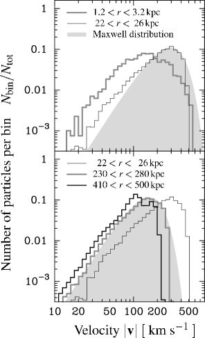
Figure 2: The distribution of the absolute value of the particle velocities $|\mathbf{v}|$ within spherical shells for the galaxy-sized halo Gal. The distributions shown in the upper panel are taken in the shell around the radius $r_{\sigma,{\rm max}}$ with maximum dispersion and in a second shell with smaller radius. The distributions shown in the lower panel are taken in shells starting from $r_{\sigma,{\rm max}}$ to larger radii. For comparison, a Maxwell distribution is shown centered at the maximum of the velocity distribution within one of the shells.

3 Velocity dispersion as a function of the potential

A spherically symmetric halo with isotropic velocity dispersion can be described using three radial functions, e.g. density, potential and velocity dispersion. These profiles are related by the Jeans and the Poisson equation. Thus, if one profile or any supplementary relation between $\sigma,\rho$ or $\Phi$ is given, the two others are determined. An invitingly simple way to get the profiles is to assume that the velocity dispersion is constant within the virial radius. However, the numerical results indicate that the velocity dispersion has a pronounced maximum at a radius $r=r_{\sigma,\rm{max}}$. For example, the galaxy-sized halo Gal shows the maximum velocity dispersion of $155\>\mathrm{km/s}$ at the position $r\approx 30\>\mathrm{kpc}$. In contrast the dispersion is only $90\>\mathrm{km/s}$ at the virial radius and to $80\>\mathrm{km/s}$ at the innermost ($r\approx 1\>\mathrm{kpc}$) radius.

On the basis of the numerical results we make an heuristic ansatz for the relation between the velocity dispersion and the potential at a given radius. Physical arguments which lead to this ansatz are discussed in Sec. 4. We approximate the dispersion as a function of the potential. This can be done because the potential increases monotonically with radius and, consequently, a one-to-one mapping between radius and potential must exist. The data can be approximated, see Fig. 3, by the relation

$$\sigma_{r}^{2} = a\left(\frac{\Phi}{\Phi_{\rm{out}}}\right)^{\kappa}\left(\Phi_{\rm{out}}-\Phi\right),$$ (3)

where $a$, $\kappa$ are free parameters and $\Phi_{\rm{out}}$ is the maximum potential reached for large radii. We denote this relation between radial velocity dispersion and potential in the following as VDPR. Since an arbitrary constant value can always be added to the potential we have set $\Phi(0)=0$. This normalization of the potential is used throughout this paper. We perform least-square fits to the data of the different halos up to radii of about two times the virial radius. Some of the halos have a companion or substructures which results in a narrow peak in the dispersion profile, e.g. halo Cl10. We exclude those peaks from the approximation if they are beyond the virial radius. The mean values obtained for the dimensionless parameters are $a=0.29\pm 0.04$ and $\kappa=0.41\pm 0.03$, where the errors are standard deviations.

The primary halo-specific parameter is the outer potential $\Phi_{\rm{out}}$. Also the parameters $a$ and $\kappa$ vary, but their scatter is small. It may be caused by substructures still present in the halo, imperfect relaxation, or even nearby structures which disturb the spherical symmetry. The smallness of the scatter may indicate that perfectly relaxed halos have only one free parameter, namely the outer potential. Consequently the VDPR may be considered to be equivalent to an equation-of-state since it gives the velocity dispersion as a function of the local potential, independent of the radius. On the other hand it incorporates global properties, namely the difference of the local potential to the central and to the outer potential. This reflects that the local particle-particle interaction is small and particles do not significantly exchange energy. Therefore, the local velocity dispersion must depend on the global properties. However, if for all perfectly relaxed halos both parameters $a$ and $\kappa$ are the same, the VDPR may serve as an additional equation which allows to close the system of Jeans and Poisson equation.

4 Velocity distribution in spherical shells

The VDPR consists apparently of two parts. The first factor $(\Phi/\Phi_{\rm{out}})^{\kappa}$ is dominant in the center of the halo whereas the second factor $\left(\Phi_{\rm{out}}-\Phi\right)$ is dominant in the outer region. Also the shape of the velocity probability density function (p.d.f.) in a shell with a small radius differs significantly from the shape in a shell with a large radius.

In Fig. 2 we provide the velocity p.d.f. determined within several spherical shells of the galaxy-sized halo Gal. Let us first consider the velocity p.d.f. $h(|\mathbf{v}|,r)$ in the upper panel in a shell around $22<r<26\>\mathrm{kpc}$ close to the radius $r_{\rm{\sigma,max}}$, where the velocity dispersion reaches its maximum. In comparison to a Maxwellian distribution the velocity p.d.f. $h(|\mathbf{v}|,r_{\rm{\sigma\,max}})$ is flatter at the small-velocity-tail and shows a steep break towards high velocities. The second p.d.f. for the shell shown in the upper panel has a radius much smaller than $r_{\rm{\sigma,max}}$. The velocity p.d.f. is much broader compared with a Maxwellian distribution. The probability peaks at $\approx 100\>\mathrm{km/s}$. Albeit there are also particles with velocities $\gtrsim 300\>\mathrm{km/s}$ – but below the escape velocity – the probability to find a particle with such a large velocity is very small near the center of the halo. This effect could be due to two reasons: first, the angular momentum of a high velocity particle must be very small to get close to the center and second, such a particle spends only very little time along its orbit near the center. Thus the probability to find particles with a high velocity decreases towards the center of the halo, whereas the orbit of slow particles is entirely in the vicinity of the center. Thus the potential well acts to concentrate slow particles in the central regions. Since there is no characteristic radius for this concentration process one may expect that the velocity dispersion scales at small radii in a self-similar manner with the potential, i.e. $\sigma_{r}^{2}\propto\Phi^{\kappa}$. This is represented by the first factor of the VDPR.

Let us now consider the shape of the velocity p.d.f. within shells around and above the virial radius, see Fig. 2, lower panel. With increasing radii of the shells the entire distribution shifts to smaller velocities. The shape of the velocity p.d.f. itself almost does not change. The probability distribution for small velocities, i.e. below the maximum of the distribution $v_{\rm{max}}$, converges to the Maxwellian distribution. For larger velocities the steep break is still present. An obvious reason for the shift is that the kinetic energy decreases when a particle moves out of the potential well. This implies that the characteristics of the velocity p.d.f., e.g. the position of the maximum velocity $v_{\rm{max}}(r)$ and the velocity dispersion $\sigma(r)$, depend directly on the potential $\Phi(r)$. Particles having velocities different from zero for $r\to\infty$, would leave the halo, i.e. they are not bound. Consequently the dispersion should vanish for large radii for an isolated halo with no additional matter around. Thus, interpreting the shift of the velocity p.d.f. as a result of the effective potential well and assuming that the shape of the p.d.f. is constant for all radii suggests a dependence between dispersion and potential according to $\sigma^{2}(r)\propto(\Phi_{\rm{out}}-\Phi(r))$ at large radii. This is represented by the second factor in the VDPR.

Figure 3: The dependence of the radial velocity dispersion $\sigma_{r}^{2}/\Phi_{\rm{out}}$ on the potential $\Phi/\Phi_{\rm{out}}$. The data obtained from the simulations are approximated by the VDPR (3).

label	Code	$r_{\rm{virial}}$	$M_{\rm{virial}}$	$N_{\rm{virial}}$	$c$	$n$	$\Phi_{\rm{out}}$	$\kappa$	$a$
		$[{\>\mathrm{Mpc}}]$	$[{\>M_{\odot}}]$				$[\rm{km^{2}/s^{2}}]$
Gal	ART	0.25	$9.2\times 10^{11}$	1066000	7.4	1.11	$1.8\times 10^{5}$	0.45	0.33
ClA	Gad	0.90	$7.0\times 10^{13}$	1031000	8.8	1.17	$2.8\times 10^{6}$	0.44	0.28
Cl6	ART	1.52	$1.46\times 10^{14}$	646000	3.6	1.54	$5.2\times 10^{6}$	0.41	0.23
Cl6b	Gad	1.30	$1.34\times 10^{14}$	590000	3.6	1.47	$5.2\times 10^{6}$	0.41	0.24
Cl7	ART	1.27	$1.23\times 10^{14}$	541000	5.2	1.14	$3.8\times 10^{6}$	0.37	0.29
Cl5	ART	1.19	$1.02\times 10^{14}$	452000	5.0	1.12	$3.3\times 10^{6}$	0.41	0.33
Cl10	ART	0.97	$5.59\times 10^{13}$	247000	5.7	1.27	$2.7\times 10^{6}$	0.38	0.28
Cl9	ART	0.90	$4.38\times 10^{13}$	193000	8.9	0.99	$2.4\times 10^{6}$	0.47	0.34
Cl12	ART	0.77	$2.79\times 10^{13}$	123000	3.5	1.46	$1.6\times 10^{6}$	0.40	0.29
Mean								0.41	0.29

Table 1: Parameters of the halos obtained by high resolution $N$-body simulations. The virial radius is determined according to $M_{\rm{vir}}\>/\>(3/4)\pi r_{\rm{vir}}^{3}=178\,\Omega_{0}^{0.45}\rho_{\rm{crit}}$, where $\rho_{\rm{crit}}$ denotes the critical density for a flat universe, see Eke et al. (1998) The density profile of the halos is approximated using a least-square fit to the (logarithmic) density values by a generalized NFW-profile Eq. (1). The concentration is given by $c=r_{\rm{vir}}/r_{s}$. The relation between the radial velocity dispersion $\sigma_{r}^{2}$ and the gravitational potential is approximated by the VDPR (3) using a least-square fits with the free parameters $a$, $\kappa$ and $\Phi_{\rm{out}}$.

5 Asymptotic profiles

We now consider the asymptotic behavior of the radial profiles at small, $r\ll r_{s}$, and at large radii, $r\gg r_{s}$.

First we discuss the outer region, where the dispersion can be approximated by $\sigma_{r}^{2}|_{r\gg r_{s}}=a\,(\Phi_{\rm{out}}-\Phi(r))$. Using the Jeans equation allows we can relate the factor $a$ to the slope of density profile. We assume isotropic dispersion, substitute the radial dispersion in the Jeans equation by the potential, integrate the Jeans equation and finally obtain the relation

$$\left.\rho(\Phi)\,\right|_{r\gg r_{s}} = c\>(\Phi_{\rm{out}}-\Phi)^{\gamma},\qquad\gamma=(1-a)/a.$$ (4)

Since, both, $(\Phi_{\rm{out}}-\Phi)$ and the density $\rho$, are monotonically decreasing functions for dark matter halos, the exponent must be positive. Therefore, the factor $a$ has to be in the range $0<a<1$. We can constrain $a$ further by inserting Eq. (4) into the Poisson equation. This results in the Lane-Emden equation (Binney & Tremaine, 1987)

$$\frac{1}{r^{2}}\frac{\rm{d}}{\rm{d}r}\left\{r^{2}\frac{\rm{d}}{\rm{d}r}(\Phi_{\rm{out}}-\Phi)\right\}+4\pi Gc(\Phi_{\rm{out}}-\Phi)^{\gamma} = 0.$$ (5)

One solution of the Lane-Emden equation is a power-law for the relative potential

$$(\Phi_{\rm{out}}-\Phi) \propto r^{-m},\qquad m=2/(\gamma-1)$$

and with Eq. (4) also for the density

$$\left.\rho\right|_{r\gg r_{s}}\>\propto\>(\Phi_{\rm{out}}-\Phi)^{\gamma} \propto r^{-n},\qquad n=2\gamma/(\gamma-1)=(2-2a)/(1-2a).$$

In order to obtain a solution for a finite mass halo the slope of density profile must be sufficiently steep, namely $n>3$. Therefore, the factor $a$ must be in the range

$$1/4<a<1/2.$$ (6)

Note the asymptotic slope of the NFW-profile, $n(r\to\infty)=3$, results from $a=1/4$. The simulations show that the anisotropy of the velocity dispersion increases with radius and amounts to $\beta\approx 0.3$ at the virial radius. This anisotropy affects the allowed parameter range for $a$: Integrating the Jeans equation under the condition of a constant anisotropy parameter $\beta$ leads to

$$\left.\rho(\Phi,r)\,\right|_{r\gg r_{s}} = c^{\ast}\>(\Phi_{\infty}-\Phi)^{\gamma}\>r^{-2\beta}.$$ (7)

Inserting this relation again into the Poisson equation allows us to find power-law solutions for the potential and the density

$$(\Phi_{\infty}-\Phi) \propto r^{-m},\qquad m=2(1-\beta)/(\gamma-1)$$

$$\left.\rho\right|_{r\gg r_{s}} \propto r^{-n},\qquad n=2(\gamma-\beta)/(\gamma-1)=2(1-a-a\beta)/(1-2a).$$

Therefore, the factor $a$ has to be in the range $1/(4-2\beta)<a<1/2$. Given the positive anisotropy by the simulations, this narrows the possible parameter range for $a$. Thus, supposing that the outer asymptotic slope of the density profile is restricted by the demand of a finite halo mass even for $r\to\infty$, the parameter $a$ has to be in the given narrow range. The halos analyzed here fulfill this condition even if they have to be truncated at a radius where the ambient, infalling matter becomes dominant.

Let us now consider the central part of the halos. The slope of the inner profile is uncertain from simulations because of the lack of force resolution and also because of the poor particle statistics. Therefore, it is still an open question whether an inner asymptote for the radial density profile exists and whether it is possible to determine its power index by numerical simulations. We make the weaker assumption that the radial velocity dispersion at sufficiently small radii is given by a power-law with respect to the potential

$$\left.\sigma_{r}^{2}(\Phi)\,\right|_{r\ll r_{s}} = a\,\Phi^{\kappa}\,\Phi_{\rm{out}}^{1-\kappa}.$$ (8)

In the same manner as described above, we insert the relation (8) into the Jeans equation, perform the integration and obtain

$$\left.\rho(\Phi)\,\right|_{r\ll r_{s}} = \rho_{0}\;\left(\frac{\Phi}{\Phi_{\rm{out}}}\right)^{-\kappa}\exp(-\frac{(\Phi/\Phi_{\rm{out}})^{1-\kappa}}{a(1-\kappa)}),$$ (9)

where $\rho_{0}$ is a free scaling constant. For $\kappa>1$ the assumption of a power-law with respect to $r$ for $\Phi$ would result in an exponential-like singularity of the density and infinite mass at final radii. In order to avoid this, the exponent $\kappa$ has to be within the range

$$0<\kappa<1.$$ (10)

Restricting $\kappa$ in this way the exponential term goes to unity at $\Phi\to 0$ at sufficient small radii, i.e. $(\Phi/\Phi_{\rm{out}})^{1-\kappa}\ll a(1-\kappa)$ and the inner asymptotic profile for the density is given by

$$\left.\rho(\Phi)\,\right|_{r\ll r_{s}} = \rho_{0}\;\left(\Phi/\Phi_{\rm{out}}\right)^{-\kappa}.$$ (11)

Note, for any $\Phi$ sufficiently small with respect to $\Phi_{\rm out}$ the asymptote Eq. (8) has the form of a power-law. In contrast, the density approaches the asymptotic behavior not until $(\Phi/\Phi_{\rm{out}})^{1-\kappa}\ll a(1-\kappa)$. In particular, if $\kappa$ is allowed to get close to unity, this latter condition becomes a very strong restriction and is valid only for very little potential values. Thus, the power-law like asymptote for $\sigma_{r}^{2}$ can be adopted much further out from the halo center. Having this in mind below we will be able to draw conclusions with respect to the density profile near the halo center. The power-law ansatz $\Phi\propto r^{m}$ provides a solution for the radial profiles. More precisely, by inserting the ansatz into the Poisson equation we can determine the free constants. For the profiles we obtain

$$\left.\Phi(r)\,\right|_{r\ll r_{s}} = \Phi_{\rm{out}}\;\left(r/r_{0}\right)^{2/(1+\kappa)}$$ (12)

$$\left.\rho(r)\,\right|_{r\ll r_{s}} = \rho_{0}\;\left(r/r_{0}\right)^{-2\kappa/(1+\kappa)},$$ (13)

with

$$r_{0}^{2} = \frac{1}{2\pi G}\;\frac{3+\kappa}{(1+\kappa)^{2}}\frac{\Phi_{\rm{out}}}{\rho_{0}}.$$ (14)

The free, halo-specific parameters for the inner asymptotes are $\Phi_{\rm{out}}$ and $r_{0}$ (or $\rho_{0}$). In the next section we compute the density profiles by integrating the basic equations. The integration will be performed starting from the small radius $r_{0}$ up to large radii, where the value $\Phi_{out}$ will be reached. The inner asymptotes given above allows us to calculate the necessary inner boundary conditions at $r_{0}$.

Figure 4: Integration of the Jeans equation (2). The halos Gal, ClA and Cl6 (triangles, circles and squares, respectively) are integrated using the VDPR (3) with the mean values for $a$ and $\kappa$ given in Tab. 1. The profiles are integrated for isotropic velocity dispersion, $\beta=0$, (dashed line) and for an anisotropy according to $\beta=0.27\Phi/\Phi_{\rm{out}}$, see Fig. 1. Initial conditions are calculated from Eqs. (12) and (13). The halo-specific values $\Phi_{\rm{out}}$ are taken from Tab. 1. For the scale radius $r_{0}$ we obtained from the dispersion profile $\sigma_{r}^{2}(r)$ the values $0.025\>\mathrm{Mpc}$, $0.12\>\mathrm{Mpc}$ and $0.13\>\mathrm{Mpc}$ for the halos Gal, ClA and Cl6, respectively.

6 Integrating the Jeans equation

Using the VDPR we can compute the profiles for a given halo, defined by two parameters, e.g. $\Phi_{\rm{out}}$ and $r_{0}$. The inner asymptotes are used to set the initial conditions. The profiles are obtained by integrating the set of ordinary differential equations

$$\frac{dM}{dr} = 4\pi\rho(r)r^{2}$$

$$\frac{d\Phi}{dr} = G\>\frac{M}{r^{2}}$$

$$\frac{d\sigma_{r}^{2}}{dr} = a\>\frac{d\Phi}{dr}\>\left(\frac{\Phi}{\Phi_{\rm{out}}}\right)^{\kappa}\left\{\kappa\frac{\Phi_{\rm{out}}}{\Phi}-\kappa-1\right\}$$

$$\frac{d\rho}{dr} = -\frac{\rho}{\sigma_{r}^{2}}\left\{\frac{d\sigma_{r}^{2}}{dr}+\frac{d\Phi}{dr}+\frac{2\beta\sigma_{r}^{2}}{r}\right\}$$

using a Runge-Kutta method. We compare the profiles obtained in this way with those from the numerical simulations. The parameter $\Phi_{\rm{out}}$ was already calculated by approximating the VDPR, see Tab. 1. We choose $r_{0}$ as second free parameter, since it causes only a stretch along the radial axis. This parameter can easily be adjusted by approximating the maximum position in the dispersion profile $\sigma_{r}^{2}(r)$. First, we assume that the velocity dispersion is isotropic, $\beta=0$. The resulting density profiles approximate roughly the results from the simulations. Clear deviations occur in the fringes of the halo. This are the regions where considerable anisotropy in the velocity dispersion is present. The anisotropy can be reasonably approximated by $\beta=\beta_{0}\Phi/\Phi_{\rm{out}}$ with $\beta_{0}\approx 0.27$. After integration, this clearly leads to a better concordance of the density profiles, see Fig. 4. For the fit of $\beta$ a dependence on the potential $\Phi$ was assumed in order to avoid the implementation of additional parameters. It can be easily seen that $\beta$ roughly follows the shape of $\Phi$, see Fig. 1. In addition, the results are almost insensitive with respect to variations of the dependence $\beta$ on $r$ as long as $\beta$ is a monotonic function.

For the halo Cl6, the integration of the differential equations leads still only to a poor approximation of the numerical results. This halo shows clear signs for undergoing still a merging process. The dispersion profile shows a peak at $\approx 1/8\,r_{\rm{vir}}$, which is caused by a remnant of a merger between the cluster and a group about $1\;\rm{Gyr}$ ago. Thus this halo is still in the process of relaxation and therefore, can be only roughly approximated by spherical, relaxed system.

The profiles of the halos ClA and Gal are recovered by the integration using the mean over all halos for the parameters $a$ and $\kappa$. However, all profiles obtained from the simulations are slightly steeper in the center than the integrated curves. Dekel et al. (2002) found that the inner profiles of disturbed halos are steepened. Therefore, a more cuspy central profile, compared to a perfectly relaxed system, may be caused by some recent merger activity.

The integrated profiles show a sharp break for radii much larger than the virial radius. They do not show the asymptotic density profile expected from the discussion in Sec. 5. This is due to the fact that the outer potential $\Phi_{\rm{out}}$ is reached at a finite radius, at which the dispersion and the density vanishes. However, since the radius where the dispersion vanishes is much larger than the virial radius of the considered halos, this outer slope cannot be determined by simulations designed to investigate structure formation.

7 Discussion and conclusion

The numerous numerical studies of the structure of dark matter halos indicate that perfectly virialized systems show presumably a universal density profile. The latter can be approximated reasonably well by the NFW-profile or a generalized version of it. Similarly we have introduced the relation between velocity dispersion and potential Eq. (3) (VDPR): it characterizes the profile by very few parameters. In contrast to the approximations of the density profiles the VDPR is implicit in the sense that it as a function of the potential instead of the radius. However, by introducing the VDPR we can put restrictions even on the inner asymptotic slope of, both, the velocity dispersion profile and the density profile. The data can be approximated very well by the newly introduced VDPR. Almost all halos clearly show a power-law for $\sigma_{r}^{2}(\Phi)\propto\Phi^{\kappa}$ near the center, the best resolved halos do so over one order of magnitude. We suppose that the obtained exponent $\kappa$ reflects also the inner asymptotic slope of $\sigma_{r}^{2}(\Phi)$. As a result, the innermost density profile power index $n$ is related to $\kappa$ by $n=2\kappa/(1+\kappa)$. Using the mean value $\kappa=0.41$, determined from all presented simulations we get $n=0.58$. The obtained standard deviation $\Delta\kappa=0.03$ permits only a negligible variation of the exponent $n$. Thus, our prediction for $n$ is below the theoretical prediction by Taylor & Navarro (2001). They argued that the inner asymptotic slope is given by $n=0.75$. Our result also indicates that the innermost slope of the density profiles is less steep than that obtained from the density profiles directly. This is not a discrepancy since the prediction $n=0.58$ is valid for scales smaller than those which are currently resolved by numerical simulations. Eq. (9) indicates that the density profile may steepened by an exponential term in a range where the velocity dispersion profile already follows a power-law. The density profile only becomes a power-law if $(\Phi/\Phi_{\rm{out}})^{1-\kappa}\ll a(1-\kappa)$ is fulfilled. For instance, the impact of the exponential term becomes smaller than 10% if the potential is below $0.001\times\Phi_{\rm out}$, using the obtained values for $\kappa$ and $a$.

In a theoretical analysis of all possible asymptotes Mücket & Hoeft (2003) found that $\kappa$ should be in the range $0<\kappa<1/3$. Therefore, the inner asymptotic slope of the density profile should be as low as $n<0.5$. Our numerical results are close to this theoretical predictions. Possible reasons for the 20% higher value of $\kappa$ could be too strong assumptions in the theoretical analysis or steepening of the central density profile during relaxation. In fact, it is still uncertain to which degree dark matter halos are actually relaxed. During the cosmological evolution halos merge frequently and show almost always substructures. Therefore, the present substructure may have impact on the resulting profiles. Nevertheless it is assumed that virialization has occured to a high degree and the halo configuration obeys the Jeans equation. The sample of halos we considered contains very relaxed halos, e.g. the halo Gal, as well as halos with clear deviations from relaxation, e.g. the halo Cl6. Dekel et al. (2002) found that ongoing merging enforces a central cusp, consequently we may have overestimated the mean value of $\kappa$ to some extent.

Our numerical results do not indicate any significant variation of the exponent $\kappa$ towards the center, see Fig. 3. Only in the case of the highest resolved halo Gal a trend of profile flattening can be noticed. Generally, a core with constant velocity dispersion might exist one a sub-resolution scale. The existence of such a core would weaken the restrictions for $\kappa$. However, the apparent inner constancy of $\kappa$ in the numerical simulations rather points to the existence of a power-law asymptote.

A further benefit of analyzing the VDPR is that this relation enables the determination of the leading processes responsible for the quite universal halo density profiles. The VDPR consists of two parts, the power-law $\Phi^{\kappa}$ and the relative potential $\Phi_{\rm{out}}-\Phi$. The latter can be understood as the gain in energy of the particles falling into the potential well. Utilizing the virial theorem $2T(r)=U(r)$, where $T(r)=(1/2)\sum\nolimits_{r<r_{i}<r+\Delta r}m_{i}v_{i}^{2}$ and $U(r)=\sum\nolimits_{r<r_{i}<r+\Delta r}m_{i}(\Phi_{\rm{out}}-\Phi)$ and assuming isotropy for the velocity dispersion, $3\sigma_{r}^{2}=v_{i}^{2}$ we obtain $\sigma_{r}^{2}=(1/3)(\Phi_{\rm{out}}-\Phi)$. The factor 1/3 is very close to the value $a=0.29$. Dark matter halos, therefore, can be considered to be locally virialized in their outer region. This leads to the observed, steep outer profiles. In the inner region of the halo the additional factor $\Phi^{\kappa}$ occurs, which may be attributed to the motion of relatively slow particles concentrated within the central potential well. Consequently, slow particles are more likely to be found in the center. This argument is scale-independent and should therefore result either in a power-law for $\sigma_{r}^{2}(\Phi)$ or in a dispersion core in the center of the halo. The characteristic and universal density profiles are a result of these two mechanisms, which do neither depend on the history of the halo formation nor on the cosmological environment. For a perfectly relaxed system an universal density profile should be expected.

In summary, we have shown that the radial velocity dispersion can be approximated well by the VDPR as a function of the potential. We have provided physical arguments for the analytical form of the VDPR. The numerical data already obey the inner power-law over one order in magnitude. Considering the inner asymptotics, we have shown that the density profile becomes a power-law if the potential is below $\approx 0.001\times\Phi_{\rm out}$. We conclude that the density profile can reach its asymptotic slope $n\lesssim 0.58$ only at scales smaller than those presently resolved.

8 Acknowledgment

We gratefully thank Anatoly Klypin, Gustavo Yepes and Matthias Steinmetz for providing results of numerical simulations. Most of the simulations have been performed at the Leibniz Rechenzentrum München and at the Konrad-Zuse-Zentrum für Informationstechnik Berlin.

References

- Binney & Tremaine (1987) Binney, J. & Tremaine, S. 1987, Galactic dynamics (Princeton, NJ, Princeton University Press, 1987, 747 p.)
- Binney & Evans (2001) Binney, J. J. & Evans, N. W. 2001, MNRAS, 327, L27
- Bullock et al. (2001) Bullock, J. S., Dekel, A., Kolatt, T. S., Kravtsov, A. V., Klypin, A. A., Porciani, C., & Primack, J. R. 2001, ApJ, 555, 240
- Crone et al. (1994) Crone, M. M., Evrard, A. E., & Richstone, D. O. 1994, ApJ, 434, 402
- de Blok et al. (2001) de Blok, W. J. G., McGaugh, S. S., & Rubin, V. C. 2001, AJ, 122, 2396
- Dekel et al. (2002) Dekel, A., Devor, J., & Arad, I. 2002, in ASP Conference Series: A New Era In Cosmology, Eds. T.Shanks & N. Metcalf
- Dekel et al. (2003) Dekel, A., Devor, J., & Hetzroni, G. 2003, MNRAS, 341, 326
- Dubinski & Carlberg (1991) Dubinski, J. & Carlberg, R. G. 1991, ApJ, 378, 496
- Eke et al. (1998) Eke, V. R., Navarro, J. F., & Frenk, C. S. 1998, ApJ, 503, 569
- El-Zant et al. (2001) El-Zant, A., Shlosman, I., & Hoffman, Y. 2001, ApJ, 560, 636
- Frenk et al. (1988) Frenk, C. S., White, S. D. M., Davis, M., & Efstathiou, G. 1988, ApJ, 327, 507
- Fukushige & Makino (2001) Fukushige, T. & Makino, J. 2001, ApJ, 557, 533
- Gavazzi et al. (2003) Gavazzi, R., Fort, B., Mellier, Y., Pelló, R., & Dantel-Fort, M. 2003, A&A, 403, 11
- Ghigna et al. (1998) Ghigna, S., Moore, B., Governato, F., Lake, G., Quinn, T., & Stadel, J. 1998, MNRAS, 300, 146
- Ghigna et al. (2000) —. 2000, ApJ, 544, 616
- Klypin et al. (2001) Klypin, A., Kravtsov, A. V., Bullock, J. S., & Primack, J. R. 2001, ApJ, 554, 903
- Kravtsov et al. (1997) Kravtsov, A. V., Klypin, A. A., & Khokhlov, A. M. 1997, ApJS, 111, 73
- Łokas & Hoffman (2000) Łokas, E. L. & Hoffman, Y. 2000, ApJ, 542, L139
- McGaugh & de Blok (1998) McGaugh, S. S. & de Blok, W. J. G. 1998, ApJ, 499, 66
- Moore et al. (1998) Moore, B., Governato, F., Quinn, T., Stadel, J., & Lake, G. 1998, ApJ, 499, L5
- Moore et al. (1999) Moore, B., Quinn, T., Governato, F., Stadel, J., & Lake, G. 1999, MNRAS, 310, 1147
- Mücket & Hoeft (2003) Mücket, J. P. & Hoeft, M. 2003, A&A accepted
- Navarro (2001) Navarro, J. F. 2001, in Invited review presented at IAU Symposium 208, Astrophysical SuperComputing using Particles, J. Makino & P.Hut, eds, 10680–+
- Navarro et al. (1996) Navarro, J. F., Frenk, C. S., & White, S. D. M. 1996, ApJ, 462, 563+
- Navarro et al. (1997) —. 1997, ApJ, 490, 493+
- Nusser & Sheth (1999) Nusser, A. & Sheth, R. K. 1999, MNRAS, 303, 685
- Power et al. (2003) Power, C., Navarro, J. F., Jenkins, A., Frenk, C. S., White, S. D. M., Springel, V., Stadel, J., & Quinn, T. 2003, MNRAS, 338, 14
- Quinn et al. (1986) Quinn, P. J., Salmon, J. K., & Zurek, W. H. 1986, Nature, 322, 329
- Salucci & Burkert (2000) Salucci, P. & Burkert, A. 2000, ApJ, 537, L9
- Seitz et al. (1998) Seitz, S., Saglia, R. P., Bender, R., Hopp, U., Belloni, P., & Ziegler, B. 1998, MNRAS, 298, 945
- Sellwood (2003) Sellwood, J. A. 2003, ApJ, 587, 638
- Springel et al. (2001) Springel, V., Yoshida, N., & White, S. D. M. 2001, New Astronomy, 6, 79
- Syer & White (1998) Syer, D. & White, S. D. M. 1998, MNRAS, 293, 337
- Taylor & Navarro (2001) Taylor, J. E. & Navarro, J. F. 2001, ApJ, 563, 483
- Thomas et al. (1998) Thomas, P. A., Colberg, J. M., Couchman, H. M. P., Efstathiou, G. P., Frenk, C. S., Jenkins, A. R., Nelson, A. H., Hutchings, R. M., Peacock, J. A., Pearce, F. R., & White, S. D. M. 1998, MNRAS, 296, 1061
- van den Bosch & Swaters (2001) van den Bosch, F. C. & Swaters, R. A. 2001, MNRAS, 325, 1017
- Weinberg & Katz (2002) Weinberg, M. D. & Katz, N. 2002, ApJ, 580, 627