First stars V - Abundance patterns from C to Zn and supernova yields in the early Galaxy

In the framework of the ESO Large Programme “First Stars”, very high-quality spectra of some 70 very metal-poor dwarfs and giants were obtained with the ESO VLT and UVES spectrograph. These stars are likely to have descended from the first generation(s) of stars formed after the Big Bang, and their detailed composition provides constraints on issues such as the nature of the first supernovae, the efficiency of mixing processes in the early Galaxy, the formation and evolution of the halo of the Galaxy, and the possible sources of reionization of the Universe. This paper presents the abundance analysis of an homogeneous sample of 35 giants selected from the HK survey of Beers et al. (1992; 1999), emphasizing stars of extremely low metallicity: 30 of our 35 stars are in the range $-2.7<{\rm[Fe/H]}<-4.1$, and 22 stars have ${\rm[Fe/H]}<-3.0$. Our new VLT/UVES spectra, at a resolving power of $R\sim 45,000$ and with signal-to-noise ratios of 100-200 per pixel over the wavelength range 330 – 1000 nm, are greatly superior to those of the classic studies of McWilliam et al. (1995) and Ryan, Norris, & Beers (1996).

The immediate objective of the work is to determine precise, comprehensive, and homogeneous element abundances for this large sample of the most metal-poor giants presently known. In the analysis we combine the spectral line modeling code “Turbospectrum” with OSMARCS model atmospheres, which treat continuum scattering correctly and thus allow proper interpretation of the blue regions of the spectra, where scattering becomes important relative to continuous absorption ($\lambda<400$ nm). We obtain detailed information on the trends of elemental abundance ratios and the star-to-star scatter around those trends, enabling us to separate the relative contributions of cosmic scatter and observational/analysis errors.

Abundances of 17 elements from C to Zn have been measured in all stars, including K and Zn, which have not previously been detected in stars with [Fe/H] $<-$3.0. Among the key results, we discuss the oxygen abundance (from the forbidden [OI] line), the different and sometimes complex trends of the abundance ratios with metallicity, the very tight relationship between the abundances of certain elements (e.g., Fe and Cr), and the high [Zn/Fe] ratio in the most metal-poor stars. Within the error bars, the trends of the abundance ratios with metallicity are consistent with those found in earlier literature, but in many cases the scatter around the average trends is much smaller than found in earlier studies, which were limited to lower-quality spectra. We find that the cosmic scatter in several element ratios may be as low as 0.05 dex.

The evolution of the abundance trends and scatter with declining metallicity provides strong constraints on the yields of the first supernovae and their mixing into the early ISM. The abundance ratios found in our sample do not match the predicted yields from pair-instability hypernovae, but are consistent with element production by supernovae with progenitor masses up to 100 M_☉. Moreover, the composition of the ejecta that have enriched the matter now contained in our very metal-poor stars appears surprisingly uniform over the range $-4.0\leq{\rm[Fe/H]}<-3.0$. This would indicate either that we are observing the products of very similar primordial bursts of high-mass stars, or that the mixing of matter from different bursts of early star formation was extremely rapid. In any case, it is unlikely that we observed the ejecta from individual (single) supernovae (as has often been concluded in previous work), as we do not see scatter due to different progenitor masses. The abundance ratios at the lowest metallicities ($-4.0\leq{\rm[Fe/H]}\leq-3.0$) are compatible with those found by McWilliam et al. (1995) and later studies. However, when elemental ratios are plotted with respect to Mg, we find no clear slopes below [Mg/H] = –3, but rather, a plateau-like behaviour defining a set of initial yields.

1 Introduction

The early chemical evolution of the Galaxy is recorded in the elemental abundances in the atmospheres of its low-mass, extremely metal-poor (XMP) stars. In the present Galaxy such stars are quite rare, especially the most metal-deficient examples. In particular, no star completely without heavy metals (a Pop III star) has been observed to date, although the recent discovery of a star with [Fe/H] = –5.3 (HE 0107-5240; Christlieb et al. 2002) proves that extreme examples of Pop II stars can still be found.

One simple explanation for the present lack of true zero-metallicity stars would be the early production of substantial amounts of metals by very massive, primitive zero-metal objects (Pop III stars). The lack of metals in such objects suggests that they should have formed with an Initial Mass Function (IMF) very different from that observed at present, either biased towards higher masses (e.g. Omukai & Nishi ON99 (1999); Bromm, Coppi, & Larson BCL99 (1999)), or with a bimodal shape (Nakamura & Umemura NU00 (2000)). The existence of zero-metal, very massive stars is postulated because such objects are able to avoid the huge radiation pressure-driven mass loss predicted for very massive stars with significant metal content (e.g., Larson L99 (1999); Abel, Bryan, & Norman ABN00 (2000); Baraffe, Heger & Woosley HW02 (2002)). Such stars are expected to play a role not only in the first episodes of heavy-element nucleosynthesis, but also in the early reionization of the Universe (Kogut et al. KSB03 (2003)). It remains possible, however, that the first stars included substantial numbers of more classical O-type stars (up to $30-60M_{\odot}$).

According to existing models, the heavy-element yields produced by these two varieties of progenitor stars, and their ability to expel these elements into the ISM, differ from one another in a number of ways. For example, a strong “odd/even” effect and low [Zn/Fe] ratios are expected in the ejecta of very massive objects exploding as pair-instability supernovae (PISN), contrary to what is expected to emerge from lower mass, classical supernovae. Hence, precise elemental abundance ratios in extremely metal-poor stars should provide a powerful means to discriminate between these two kinds of “first stars.”

A main aim of the present programme is to obtain precise determinations of the elemental abundances in extremely metal-poor stars, since these abundances reflect the yields of the first supernovae – perhaps even of a single one according to Audouze & Silk (AS95 (1995)) and Ryan et al. (RNB96 (1996)); see also Shigeyama & Tsujimoto (ST98 (1998)), Nakamura et al. (NUN99 (1999)), Chieffi & Limongi (CL02 (2002)), and Umeda & Nomoto (UN02 (2002)). However, whether or not they are associated with single supernovae, precise abundances provide very useful constraints on model yields of the first supernovae, which are not yet well understood.

The most reliable information is clearly to be obtained from a homogeneous and systematic determination of elemental abundances in large samples of such stars, so that reliable trends of the abundance ratios with metallicity may be determined. Such trends may then be interpreted in terms of variable (or constant) yields as a function of time, of the progenitor masses, and/or of the metallicity of the ISM in the early Galaxy. Moreover, high-quality data and a careful, consistent analysis reduce the contribution of systematic and random errors to the star-to-star scatter of the derived abundance ratios, enabling a much better estimate of their intrinsic (cosmic) scatter and thereby constraining the efficiency of the mixing processes in the primitive halo.

Even after decades of dedicated searches, the number of XMP stars that are sufficiently bright to be studied at sufficiently high spectral resolution, even with large telescopes, remains small. The present paper reports observations of the first half of a sample of roughly 70 XMP candidates, including both turn-off and giant stars and selected from the HK survey of Beers and colleagues (Beers et al. BPS92 (1992); Beers 1999).

Several papers have already been published on particularly interesting individual stars from this programme: Hill et al. (HPC02 (2002)), Depagne et al. (DHS02 (2002)), François et al. (FDH03 (2003)), and Sivarani et al. (SBM03 (2003)). In contrast, we discuss here the derived element abundances, from carbon to zinc, for our entire homogeneous sample of 35 very metal-poor giants. Among these, 22 have metallicities ${{\rm[Fe/H]}<-3.0}$ and thus qualify as XMP stars.

We have carried out an analysis in a systematic and homogeneous way, based on the highest-quality data obtained to date. Compared to previous work (e.g. McWilliam et al. MPS95 (1995); Ryan et al. 1996), our spectra cover a substantially larger wavelength range at much higher spectral resolution and S/N ratios, allowing for a significant leap forward in the accuracy of the derived elemental abundances (Sect. 2). These abundances were derived with particular care from the spectra, supplemented by new photometric data in several colours and using state-of-the-art model atmospheres (Sect. 3). Moreover, we study important elements, such as O, K, and Zn which were not analyzed in previous works. The derived elemental abundances and abundance ratios are presented in Sect. 4, the results are discussed in section 5, and conclusions are drawn in section 6.

Table 1: Log of the UVES observations. The S/N ratio per pixel is given for three representative wavelengths. (Due to the large number of pixels in each resolution element, the S/N ratios of the table need to be multiplied by a factor of 1.3 in order to compare them to the values available in the literature)

Star Name			Slit	Total Exposure Time
		Date of	Width	Blue	Yellow	Red	S/N	S/N	S/N
	V	Observation	”	396nm	573nm	850nm	400nm	510nm	630nm
1 HD 2796	8.51	Oct 2000	1.0	1800	1300	400	250	390	550
2 HD 122563	6.20	Jul 2000	1.0				250	430	670
3 HD 186478	9.18	Oct 2000	1.0	800	400	400
4 BD +17:3248	9.37	Oct 2000	1.0	2700	2700	1200	160	290	310
–		Jun 2001
–		Sep 2001
5 BD –18:5550	9.35	Oct 2000	1.0	1800	1200	600	220	410	630
–		Sep 2001
6 CD –38:245	12.01	Jul 2000	1.0	7200	3600	3600	150	150	200
–		Aug 2000
7 BS 16467–062	14.09	Jun 2001	1.0	3600	3600		90	140	170
–		Jul 2001		7200	3600	3600
8 BS 16477–003	14.22	Jun 2001	1.0	14400	7200	7200	90	130	170
9 BS 17569–049	13.36	Jun 2001	1.0	9600	6600	3000	120	170	260
10 CS 22169–035	12.88	Oct 2000	1.0	7200	3600	3600	150	210	280
11 CS 22172–002	12.73	Oct 2000	1.0	7494	3600	3900	130	200	330
12 CS 22186–025	14.24	Oct 2001	1.0	10800	7200	3600	95	140	190
13 CS 22189–009	14.04	Oct 2000	1.0	7200	3600	3600	90	150	120
14 CS 22873–055	12.65	May 2001	1.0	7200	3600	3600	140	150	200
–		Sep 2001
15 CS 22873–166	11.82	Oct 2000	1.0	5400	2700	2700	160	240	300
16 CS 22878–101	13.73	Jul 2000	1.0	14400	7200	7200	85	100	120
17 CS 22885–096	13.33	Jul 2000	1.0	15835	9184	6600	160	250	410
–		Aug 2000
18 CS 22891–209	12.17	Oct 2000	1.0	5400	2700	2700	160	200	350
19 CS 22892–052	13.18	Sep 2001	1.0	7200	3600	3600	140	130	190
20 CS 22896–154	13.64	Oct 2000	1.0	12600	7200	5400	110	230	200
21 CS 22897–008	13.33	Oct 2000	1.0	10800	5400	5400	100	170	180
22 CS 22948–066	13.47	Sep 2001	1.0	7200	3600	3600	100	130	130
23 CS 22949–037	14.36	Aug 2000	1.0	30000	19200	10800	110	180	170
–		Sep 2001
24 CS 22952–015	13.28	Oct 2000	1.0	10200	4800	5400	150	220	250
25 CS 22953–003	13.72	Sep 2001	1.0	13500	9900	3600	140	160	210
26 CS 22956–050	14.27	Sep 2001	1.0	9000	5400	3600	75	95	130
27 CS 22966–057	14.32	Sep 2001	1.0	9000	5400	3600	80	105	120
28 CS 22968–014	13.72	Oct 2000	1.0	14100	8700	5400	150	220	240
29 CS 29491–053	12.92	Oct 2001	1.0	5800	2900	2900	140	205	230
30 CS 29495–041	13.34	Jun 2001	1.0	7200	3600	3600	115	130	170
–		Sep 2001
31 CS 29502–042	12.71	Oct 2000	1.0	13500	9900	3600	290	310	330
–		Sep 2001
32 CS-29516–024	13.59	Jun 2001	1.0	3600	3600		140	205	230
33 CS 29518–051	13.02	Oct 2000	1.0	7200	3600	3600	100	150	190
34 CS 30325–094	12.33	Jul 2000	1.0	7200	6300	3600	110	220	280
–		Aug 2000
35 CS 31082–001	11.70	Aug 2000	1.0	2400	1200	1200	-*	-*	-*
–		Aug 2000	0.45	6000	3000	3000
–		Oct 2000	0.45	25200	10800	14400
* for CS 31082–001 the details of the observations are given in Hill et al.(2002)

2 Observations and reductions

The observations were performed during several runs from April 2000 to November 2001 with the VLT-UT2 and the high-resolution spectrograph UVES (Dekker et al. DD00 (2000)). Details are presented in Table 1. Accurate coordinates for the brighter stars can be found in the SIMBAD database (http: //simbad.u-strasbg.fr/); those for other stars are given in Table LABEL:tab-coor. In this paper the names of the stars have been shortened to, for example, CS XXXXX–XXX instead of BPS CS XXXXX–XXX, where BPS is the SIMBAD abbreviation for the catalogue of Beers, Preston, & Shectman. Several stars of our sample have duplicate names; the second name is indicated in Table LABEL:tab-coor in italics .

Table 2: Precise coordinates of the BPS programme stars. Four of our stars have duplicate names. The second name is given in italics. The coordinates of the HD and BD stars of our sample can be found in SIMBAD.

	Star Name	$\alpha(2000)$	$\delta(2000)$
7	BS 16467–062	13:42:00.63	$+$17:48:40.8
	BS 16934–060	–	–
8	BS 16477–003	14:32:56.91	$+$06:46:06.9
	CS 30317–084	–	–
9	BS 17569–049	22:04:58.36	$+$04:01:32.1
10	CS 22169–035	04:12:13.88	$-$12:05:05.0
11	CS 22172–002	03:14:20.84	$-$10:35:11.2
12	CS 22186–025	04:24:32.80	$-$37:09:02.5
13	CS 22189–009	02:41:42.37	$-$13:28:10.5
14	CS 22873–055	19:53:49.78	$-$59:40:00.1
15	CS 22873–166	20:19:22.02	$-$61:30:14.9
16	CS 22878–101	16:45:31.44	$+$08:14:45.4
17	CS 22885–096	20:20:51.17	$-$39:53:30.1
18	CS 22891–209	19:42:02.16	$-$61:03:44.6
19	CS 22892–052	22:17:01.65	$-$16:39:27.1
20	CS 22896–154	19:42:26.88	$-$56:58:34.0
21	CS 22897–008	21:03:11.85	$-$65:05:08.8
22	CS 22948–066	21:44:51.17	$-$37:27:54.9
	CS 30343–064	–	–
23	CS 22949–037	23:26:29.80	$-$02:39:57.9
24	CS 22952–015	23:37:28.69	$-$05:47:56.6
25	CS 22953–003	01:02:15.85	$-$61:43:45.8
26	CS 22956–050	21:58:05.83	$-$65:13:27.1
27	CS 22966–057	23:48:57.76	$-$29:39:22.8
28	CS 22968–014	03:06:29.50	$-$54:30:32.5
29	CS 29491–053	22:36:56.30	$-$28:31:06.4
30	CS 29495–041	21:36:33.27	$-$28:18:48.5
31	CS 29502–042	22:21:48.82	$+$02:28:44.8
	CS 29516–041	–	–
32	CS 29516–024	22:26:15.35	$+$02:51:46.2
33	CS 29518–051	01:24:10.01	$-$28:15:21.0
34	CS 30325–094	14:54:39.27	$+$04:21:38.0
35	CS 31082–001	01:29:31.13	$-$16:00:45.4

A dichroic beam-splitter was used for all of the observations, permitting the use of both arms of the spectrograph simultaneously; the blue arm was centered at 396nm and the red arm at either 573 or 850nm. The resulting spectral coverage is almost complete from 330 nm to 1000 nm. The entrance slit, 1” on the sky, yielded a resolving power of $R\approx 47,000$ at 400 nm and 43,000 at 630 nm. The S/N ratios per pixel at different wavelengths are summarized in Table 1. Since there are $\approx$ 5 pixels per resolution element, these values should be multiplied by a factor 2.2 in order to obtain the S/N ratios per resolution element (and by 1.3 when comparing them to S/N values in the literature, as most other spectrographs have only 3 pixels per resolution element).

Norris et al. (NRB01 (2001)) defined a “figure of merit,” F, which is useful for comparing the quality of high-resolution spectroscopic observations, assuming the integrated signal from observed spectral features is made with the same number of pixels. They suggest that, in order to achieve significant progress in issues of importance for Galactic chemical evolution, spectra should ideally be obtained with F larger than 500. The observations presented herein have figures of merit, F, in the blue (400 nm) between 850 and 3250, and in the red (630 nm) between 650 and 2350 (F is much higher for the two bright stars HD 122563 and BD-18:5550, which have been analysed several times in the literature and were observed with particular care to check for possible systematic errors).

The $r$-process enhanced, very metal-poor star CS 31082–001 was observed with slightly different settings and slit widths to obtain higher spectral resolution and complete coverage in the blue. The details of the observations for this star are given in Hill et al. (HPC02 (2002)).

The spectra were reduced using the UVES context (Ballester et al. BMB00 (2000)) within MIDAS, which performs bias and inter-order background subtraction (object and flat-field), optimal extraction of the object (rejecting cosmic ray hits), division by a flat-field frame extracted with the same optimally weighted profile as the object, wavelength calibration and rebinning to a constant value, and merging of all overlapping orders. The spectra were then co-added and finally normalized to unity in the continuum. For the reddest spectra (centered at 850 nm), instead of correcting the image by the extracted flat-field, the object frame was divided by the flat-field frame pixel-by-pixel (in 2D, before extraction), which yields a better correction of the interference fringes that appear in these frames. An example of the spectra is given in Fig. 1.

Figure 1: An example of the reduced spectra in the region of the Ca II H and K lines, the Mg I triplet, and in the region of the forbidden oxygen line. The abscissa is the wavelength in nm. Telluric lines are indicated.

2.1 Equivalent widths

In most cases the equivalent widths (EWs) of individual lines were measured by Gaussian fitting and then employed to determine the abundances of the different elements. The equivalent widths of the lines for each star are available as an electronic file. In the cases of elements which suffer from hyperfine structure and/or molecular bands and blends, the abundances have been directly determined by spectral synthesis.

In Fig. 2 we compare our measured EWs for stars in common with several recent spectroscopic studies, e.g., McWilliam et al. (MPS95 (1995)), Carretta et al. (CGC02 (2002)), and Johnson (JJ02 (2002)). The quality of Johnson’s spectra is similar to ours, and the agreement between the two sets of measurements is excellent (standard deviation 3.6 mÅ for HD 122563, and only 2.2 mÅ when restricting the comparison to lines with EW $<30$ mÅ). The agreement with the data of Carretta et al. is also quite good (standard deviation 5.5 mÅ for CS 22878–101). When our data are compared to the equivalent widths of McWilliam et al., however, the standard deviation is larger, 10 mÅ for CS 22892–052, presumably due to the much lower resolution and S/N ratio of the McWilliam et al. spectra ($R=22,000$ and $S/N=36$).

The mean difference between our EWs and those reported in the literature is generally quite small; the regression line between our data and those of Johnson, Carretta et al., or McWilliam et al. has a slope close to one, with deviations always less than 3% and a very small zero-point shift.

Figure 2: Comparison between our EWs and those of Johnson (2002), Carretta et al. (2002), and McWilliam et al. (1995). The one-to-one relation is shown by a dashed line, the mean curve (least squares) by a full thin line. The value of the slope (a) and zero point shift (b) of the regression are given, as well as the standard deviation of the fit ($\sigma$).

The expected uncertainty in the measured equivalent widths can be estimated from Cayrel’s formula (Cay88 (1988)) :

$$\sigma_{W}={1.5\over{S/N}}\sqrt{FWHM*\delta x}$$

where S/N is the signal-to-noise ratio per pixel, FWHM is the full width of the line at half maximum, and $\delta x$ the pixel size. The predicted accuracy, $\sigma_{W}$, is 0.4mÅ for a typical S/N ratio of 150 and only 0.3mÅ for a S/N ratio of 200. These are also the weakest lines which can be detected in the spectra. However, it should be noted that this formula neglects the uncertainty on the continuum placement, as well as the uncertainty in the determination of the FWHM of the lines.

We estimate that, using homogeneous procedures for the determination of the continua and the line widths, the statistical error for weak lines is of the order of 0.6–1.0mÅ, depending on the S/N ratio of the spectrum and the level of crowding. Since the lines used in our abundance analysis are generally very weak, the error on the abundance determination depends almost linearly on the error of the measured equivalent widths.

3 Analysis and determination of the stellar parameters

Table 3: Photometry and derived temperatures for the programme stars. The V-I and V-R colours are on the Johnson system, while J-K and V-K have been transformed to the TCS system (see Alonso et al. 2001).

			Teff		Teff		Teff		Teff		Teff	Adopted
Star Name	$E_{B-V}$	B-Vo	B-V	V-Ro	V-R	J-Ko	J-K	V-Ko	V-K	V-Io	V-I	Teff
1 HD 2796	0.03	0.71	5072	0.68	4999	0.54	4907	2.23	4902			4950
2 HD 122563	0.00	0.90	4653	0.81	4586	0.61	4657	2.51	4574			4600
3 HD 186478	0.09	0.84	4726	0.76	4690	0.58	4757	2.26	4811			4700
4 BD+17:3248	0.06	0.60	5386	0.59	5238	0.47	5142	1.89	5240			5250
5 BD-18:5550	0.08	0.77	4823	0.76	4709	0.58	4745	2.58	4520			4750
6 CD-38:245	0.00	0.76	4841	0.73	4806	0.58	4739	2.36	4712	1.30	4700	4800
7 BS 16467–062	0.00	0.60	5352	0.60	5234	0.44	5278	1.89	5284	1.08	5120	5200
8 BS 16477–003	0.01	0.75	4869	0.68	5004	0.53	4937	2.24	4878	1.23	4848	4900
9 BS 17569–049	0.03	0.86	4718			0.58	4732	2.42	4662			4700
10 CS 22169–035	0.02	0.87	4706			0.59	4717	2.47	4617	1.43	4501	4700
11 CS 22172–002	0.06	0.75	4854			0.50	5034	2.24	4846	1.26	4770	4800
12 CS 22186–025	0.01	0.73	4880	0.70	4887	0.49	5087	2.16	4935	1.21	4855	4900
13 CS 22189–009	0.02	0.70	4917	0.68	4968	0.53	4901	2.18	4913			4900
14 CS 22873–055	0.03	0.90	4670	0.81	4577	0.58	4738	2.56	4537	1.45	4473	4550
15 CS 22873–166	0.03	0.94	4623	0.83	4542	0.63	4595	2.61	4495			4550
16 CS 22878–101	0.06	0.78	4816	0.69	4933	0.55	4848	2.32	4757	1.25	4792	4800
17 CS 22885–096	0.03	0.66	5146	0.67	4987	0.48	5114	2.15	4949			5050
18 CS 22891–209	0.05			0.76	4732	0.54	4894	2.42	4667			4700
19 CS 22892–052	0.00	0.78	4816	0.69	4921	0.52	4967	2.25	4837	1.27	4761	4850
20 CS 22896–154	0.04	0.58	5416	0.60	5238	0.47	5167	1.99	5161			5250
21 CS 22897–008	0.00	0.69	5052	0.69	4917	0.55	4860	2.33	4750			4900
22 CS 22948–066	0.00	0.63	5243	0.63	5117	0.50	5047	2.02	5111	1.14	4986	5100
23 CS 22949–037	0.02	0.72	4887	0.70	4901	0.52	4964	2.22	4874			4900
24 CS 22952–015	0.01	0.77	4845	0.73	4820	0.56	4845	2.34	4763			4800
25 CS 22953–003	0.00	0.67	5114	0.64	5088	0.49	5084	2.07	5046			5100
26 CS 22956–050	0.00	0.68	5083			0.53	4911	2.25	4836			4900
27 CS 22966–057	0.00	0.61	5314	0.57	5346	0.42	5371	1.78	5427	1.04	5202	5300
28 CS 22968–014	0.00	0.72	4887	0.69	4917	0.51	4981	2.27	4812			4850
29 CS 29491–053	0.00	0.84	4742			0.57	4787	2.39	4683			4700
30 CS 29495–041	0.00	0.81	4778			0.54	4866	2.35	4721			4800
31 CS 29502–042	0.00	0.68	5083			0.45	5217	2.05	5073			5100
32 CS 29516–024	0.06	0.89	4751	0.88	4430	0.58	4744	2.45	4636	1.44	4486	4650
33 CS 29518–051	0.00	0.64	5223	0.61	5208	0.46	5173	1.97	5182	1.09	5099	5200
34 CS 30325–094	0.02	0.70	4919			0.48	5100	2.15	4951	1.17	4931	4950
35 CS 31082–001	0.00	0.77	4822	0.69	4932	0.54	4877	2.21	4882	1.23	4826	4825

The abundance analysis was performed using the LTE spectral line analysis code “Turbospectrum” together with OSMARCS model atmospheres. The OSMARCS models were originally developed by Gustafsson et al. (GBE75 (1975)) and have been constantly improved and updated through the years by Plez et al. (PBN92 (1992)), Edvardsson et al. (EAG93 (1993)), and Asplund et al. (AGK97 (1997)). For a description of the most recent improvements, and the coming grid, see Gustafsson et al. GEE03 (2003). Turbospectrum is described by Alvarez & Plez (AP98 (1998)), and has recently been improved, partly for this work, especially through the addition of a module for abundance determinations from measured equivalent widths.

The abundances of the different elements have been determined mainly from the measured equivalent widths of isolated, weak lines. Synthetic spectra have only been used to determine the abundance of C and N from the CH and CN molecular bands, or when lines were severely blended (e.g., for silicon) or required corrections for hyperfine splitting (e.g., for manganese).

3.1 Determination of stellar parameters

The temperatures of the programme stars were estimated from the observed colour indices using Alonso et al.’s calibration for giants (Alonso et al. AAM99 (1999)). This calibration is based on the Infrared Flux Method (IRFM), which provides the coefficients used to convert colours to effective temperatures (T_eff).

The colours of the stars have been taken from Beers et al. (2003, in preparation), Alonso et al. (AAM98 (1998)), the 2MASS catalogue (J,H,K) (Skrutskie et al. 2MASS97 (1997); Finlator et al. 2MASS00 (2000)), or the DENIS catalogue (I,J,K) (Epchtein et al. DENIS99 (1999)).

The indices V-R and V-I, originally on the Cousins system, have been transformed (Bessell Bes83 (1983)) onto the Johnson system adopted by Alonso et al. for use with the relations T_eff vs. V-R and V-I. The 2MASS J-K and V-K indices were transformed onto the TCS (Telescopio Carlos Sanchez) system through the ESO system (Carpenter Car01 (2001)), since Alonso et al. use this system for these colours. For the “CS” or “BS” stars the colour indices have been corrected for reddening following Beers et al. (Be99 (1999)), who used Burstein & Heiles (BH82 (1982)) values, corrected for distance. This $E_{(B-V)}$ value is systematically smaller than the value computed from the Schlegel et al. (SFD98 (1998)) map by about 0.02 mags. Arce & Goodman (AG99 (1999)) found that the Schlegel et al. map overestimates the extinction in some regions, in particular when the extinction is large. For the bright stars of the sample, reddening was taken from Pilachowski et al. (PSK96 (1996)).

The adopted values of $E_{(B-V)}$ and the dereddened colours are listed in Table LABEL:tab-Phot, along with the corresponding derived temperatures. These values would be about 50K higher if the Schlegel et al. (SFD98 (1998)) values for reddening had been adopted. We note that for CS 31082–001 the temperature deduced from (V-R) is higher than the temperature found in Hill et al. (HPC02 (2002)), because in the latter paper the transformation V-R vs. temperature had been taken from McWilliam et al. (MPS95 (1995)).

The final temperatures adopted for our analysis are listed in Table LABEL:tab-Phot (column 13); 82% of the temperatures deduced from the different colours are located inside the interval $\mathrm{T(adopted)\pm 100K}$. This corresponds to a random error of about 80K ($1\leavevmode\nobreak\ \sigma$).

The microturbulent velocity, $v_{t}$, was derived from Fe I lines in the traditional manner, requiring that the abundance derived for individual lines be independent of the equivalent width of the line. Finally, the surface gravity, log $g$, was determined by requiring that the Fe and Ti abundances derived from Fe I and Fe II, resp. Ti I, Ti II lines be identical.

It should be noted that our log $g$ values may be affected by NLTE effects (overionization) and by uncertainties in the oscillator strengths of the Fe and Ti lines. Carretta et al. (CGC02 (2002)) used another method: they deduced the gravity from isochrones (Yi et al. YDK01 (2001)), and found that the abundances of iron deduced from Fe I or Fe II lines show ionization equilibrium within 0.2 dex (cf. their Table 1). For the one star we have in common with these authors (CS 22878–101), we adopted the same effective temperature (T_eff=4800K), and the agreement for log $g$ is excellent; in both cases log $g$ = 1.3 (Table 4). Hence, these two independent methods provide similar results.

The final model atmosphere parameters adopted for the stars are given in Table 4.

Table 4: Adopted model parameters (T_eff, log $g$, $v_{t}$, [Fe/H]_m) and final iron abundances [Fe/H]_c for the programme stars.

Star	Teff	log g	$v_{t}$	[Fe/H]m	[Fe/H]c
1 HD 2796	4950	1.5	2.1	-2.4	-2.47
2 HD 122563	4600	1.1	2.0	-2.8	-2.82
3 HD 186478	4700	1.3	2.0	-2.6	-2.59
4 BD +17:3248	5250	1.4	1.5	-2.0	-2.07
5 BD –18:5550	4750	1.4	1.8	-3.0	-3.06
6 CD –38:245	4800	1.5	2.2	-4.0	-4.19
7 BS 16467–062	5200	2.5	1.6	-4.0	-3.77
8 BS 16477–003	4900	1.7	1.8	-3.4	-3.36
9 BS 17569–049	4700	1.2	1.9	-3.0	-2.88
10 CS 22169–035	4700	1.2	2.2	-3.0	-3.04
11 CS 22172–002	4800	1.3	2.2	-4.0	-3.86
12 CS 22186–025	4900	1.5	2.0	-3.0	-3.00
13 CS 22189–009	4900	1.7	1.9	-3.5	-3.49
14 CS 22873–055	4550	0.7	2.2	-3.0	-2.99
15 CS 22873–166	4550	0.9	2.1	-3.0	-2.97
16 CS 22878–101	4800	1.3	2.0	-3.0	-3.25
17 CS 22885–096	5050	2.6	1.8	-4.0	-3.78
18 CS 22891–209	4700	1.0	2.1	-3.0	-3.29
19 CS 22892–052	4850	1.6	1.9	-3.0	-3.03
20 CS 22896–154	5250	2.7	1.2	-2.7	-2.69
21 CS 22897–008	4900	1.7	2.0	-3.5	-3.41
22 CS 22948–066	5100	1.8	2.0	-3.0	-3.14
23 CS 22949–037	4900	1.5	1.8	-4.0	-3.97
24 CS 22952–015	4800	1.3	2.1	-3.4	-3.43
25 CS 22953–003	5100	2.3	1.7	-3.0	-2.84
26 CS 22956–050	4900	1.7	1.8	-3.3	-3.33
27 CS 22966–057	5300	2.2	1.4	-2.6	-2.62
28 CS 22968–014	4850	1.7	1.9	-3.5	-3.56
29 CS 29491–053	4700	1.3	2.0	-3.0	-3.04
30 CS 29495–041	4800	1.5	1.8	-2.8	-2.82
31 CS 29502–042	5100	2.5	1.5	-3.0	-3.19
32 CS 29516–024	4650	1.2	1.7	-3.0	-3.06
33 CS 29518–051	5100	2.4	1.4	-2.8	-2.78
34 CS 30325–094	4950	2.0	1.5	-3.4	-3.30
35 CS 31082–001	4825	1.5	1.8	-2.9	-2.91

Figure 3: Comparison of FeI abundance for CS 22878–101 vs. excitation potential, equivalent width, and wavelength. The parameters adopted for the model are T_eff = 4800K, log $g$ = 1.3, $v_{t}$= 2.0 km s^-1, and [Fe/H]${}_{m}=-3.0$. The line at [Fe/H] = –3.29 represents the mean value of the iron abundance deduced from the Fe I lines.

Table 5: Abundance uncertainties linked to stellar parameters.

HD 122563
A: Teff=4600K, log g=1.0 dex, vt=2.0 km s-1
B: Teff=4600K, log g=0.9 dex, vt=2.0 km s-1
C: Teff=4600K, log g=1.0 dex, vt=1.8 km s-1
D: Teff=4500K, log g=1.0 dex, vt=2.0 km s-1
E: Teff=4500K, log g=0.6 dex, vt=1.8 km s-1
El.	$\Delta_{B-A}$	$\Delta_{C-A}$	$\Delta_{D-A}$	$\Delta_{E-A}$
[Fe/H]	-0.00	0.06	-0.09	-0.06
$[$O I/Fe]	-0.03	-0.06	0.04	-0.12
$[$Na I/Fe]	0.04	0.05	-0.16	0.03
$[$Mg I/Fe]	0.03	-0.01	-0.04	0.07
$[$Al I/Fe]	0.04	0.04	-0.13	0.08
$[$Si I/Fe]	0.02	0.04	-0.05	0.08
$[$K I/Fe]	0.02	-0.04	-0.02	0.01
$[$Ca I/Fe]	0.02	-0.03	0.00	0.05
$[$Sc II/Fe]	-0.02	0.02	0.04	-0.01
$[$Ti I/Fe]	0.02	-0.01	-0.09	-0.00
$[$Ti II/Fe]	-0.02	0.02	0.04	0.01
$[$Cr I/Fe]	0.02	0.05	-0.13	0.03
$[$Mn I/Fe]	0.03	0.07	-0.18	-0.03
$[$Fe I/Fe]	0.03	0.03	-0.11	0.03
$[$Fe II/Fe]	-0.03	-0.04	0.11	-0.03
$[$Co I/Fe]	0.02	0.08	-0.14	0.05
$[$Ni I/Fe]	0.03	0.07	-0.13	0.05
$[$Zn I/Fe]	-0.03	-0.07	0.04	-0.03
$[$O I/Mg I]	-0.06	-0.05	+0.07	-0.19
$[$O/Mg]∗	-0.01	+0.02	-0.14	-0.13
Note: [O/Mg]∗ = [O I/Fe II]-[Mg I/Fe I]

Table 6: Abundance uncertainties linked to stellar parameters.

CS 22948–066
A: Teff=5100K, log g=1.8 dex, vt=2.0 km s-1
B: Teff=5100K, log g=1.7 dex, vt=2.0 km s-1
C: Teff=5100K, log g=1.8 dex, vt=1.8 km s-1
D: Teff=5000K, log g=1.8 dex, vt=2.0 km s-1
E: Teff=5000K, log g=1.5 dex, vt=2.0 km s-1
El.	$\Delta_{B-A}$	$\Delta_{C-A}$	$\Delta_{D-A}$	$\Delta_{E-A}$
[Fe/H]	-0.02	0.02	-0.05	-0.11
$[$O I/Fe]	-0.01	-0.02	-0.02	-0.05
$[$Na I/Fe]	0.03	0.08	-0.04	0.05
$[$Mg I/Fe]	0.04	0.06	-0.01	0.10
$[$Al I/Fe]	0.03	0.05	-0.04	0.04
$[$Si I/Fe]	0.03	0.05	-0.05	0.04
$[$K I/Fe]	0.02	-0.02	-0.03	0.05
$[$Ca I/Fe]	0.02	-0.01	-0.02	0.05
$[$Sc II/Fe]	-0.01	0.02	0.00	-0.03
$[$Ti I/Fe]	0.02	-0.02	-0.07	-0.01
$[$Ti II/Fe]	-0.01	0.03	0.00	-0.03
$[$Cr I/Fe]	0.03	0.03	-0.06	0.02
$[$Mn I/Fe]	0.03	0.05	-0.06	0.02
$[$Fe I/Fe]	0.02	0.03	-0.06	0.02
$[$Fe II/Fe]	-0.02	-0.02	0.06	-0.01
$[$Co I/Fe]	0.03	0.02	-0.07	0.01
$[$Ni I/Fe]	0.02	0.10	-0.07	0.01
$[$Zn I/Fe]	0.01	-0.02	0.00	0.03
$[$O I/Mg I]	-0.05	-0.08	-0.01	-0.15
$[$O/Mg]∗	-0.01	-0.03	-0.13	-0.12
Note: [O/Mg]∗ = [O I/Fe II]-[Mg I/Fe I]

3.2 Validity checks

To check the validity of the model parameters (T_eff, log g, $v_{t}$) we have plotted for all the Fe I lines in each star (see Fig. 3): (i) the iron abundance as a function of the excitation potential of the line (to check the adopted temperature and the importance of NLTE effects); (ii) the abundance vs. the equivalent width of the line (to check on the microturbulence velocity); (iii) the abundance vs. wavelength (as a consistency check, which can shed light on problems linked to the synthetic spectra computations).

Using the photometrically derived T_eff we find no trend with the excitation of Fe I lines (at least when only the lines with $\chi_{ex}>1$eV are taken into account), contrary to what was reported by Johnson (2002) using Kurucz models. Johnson also found, for the most metal-poor stars of her sample, a trend of increasing abundance with decreasing wavelength. In a first approach we saw the same effect, using a spectrum synthesis code that treats continuum scattering as if it were absorption. The Turbospectrum code takes proper account of continuum scattering, with the source function written as $S_{\nu}=(\kappa_{\nu}\times B_{\nu}+\sigma_{\nu}\times J_{\nu})/(\kappa_{\nu}+\sigma_{\nu})$, consistent with the OSMARCS code. With proper treatment of continuum scattering we find no or much less correlation of abundance with wavelength.

Indeed, it turns out to be crucial to not approximate scattering by absorption. In our model with T_eff = 4600 K, log $g$ = 1.0, and [Fe/H] = –3, the ratio $\sigma/\kappa$ in the continuum opacity at the $\tau_{\lambda}=1$ level is 5.2 at $\lambda$ = 350 nm, whereas it is only 0.08 at $\lambda$ = 500 nm. At $\tau_{\lambda}=0.1$, these numbers are 57 and 3.2 respectively. In the presence of significant scattering, radiation in the continuum reflects the physical conditions of deeper, hotter layers than those at $\tau=1$ (the $J_{\nu}$ part of the source function). Neglecting this, which is equivalent to including scattering in the absorption coefficient, results in too low a flux in the continuum, and thus too weak spectral lines.

In fact, for the model above, calculations show that the continuum flux with scattering included in absorption is only 55% of its value with scattering at 350 nm, 93% at 500 nm). This forces the derived abundances towards higher values at the (short) wavelengths where scattering is important. It is thus especially important to properly account for continuum scattering when studying metal-poor stellar spectra!

For completeness, we note that in some cases we even find a slight opposite trend (decreasing abundance at shorter wavelength), which we interpret as due to NLTE effects in lines which are at least partly formed by scattering.

3.3 Stellar parameter uncertainties and associated abundance uncertainties

For a given stellar temperature, the ionization equilibrium provides an estimate of the stellar gravity with an internal accuracy of about 0.1 dex in log $g$, and the microturbulence velocity $v_{t}$  can be constrained within 0.2 km s^-1. The largest uncertainties in the abundance determination arise in fact from the uncertainty in the temperature of the stars.

First, the different indices give different temperature estimates; from Sect. 3.1 we estimate that the corresponding error is about 80 K. Another source of error is the estimation of the reddening. The error on $E_{(B-V)}$ is about 0.02 mags, corresponding to a temperature error of about 60 K. Overall, we estimate that the total error on the adopted temperatures is on the order of 100 K.

Tables 5 and 6 list the abundance uncertainties arising from each of these three sources (log $g$, $v_{t}$, and T_eff) individually (columns 2 to 4, from the comparison of models B, C and D to the nominal model labeled A) for two stars which cover much of the parameter space of our sample: HD 122563 (T_eff = 4600K, log $g$ = 1.0, $v_{t}$= 2.0 km s^-1, and [Fe/H] = –2.8, Barbuy et al. BMS03 (2003)) and CS 22948–066 (T_eff = 5100K, log $g$ = 1.8, $v_{t}$= 2.0 km s^-1, and [Fe/H] = –3.1).

Because gravity is determined from the ionization equilibrium, a variation of T_eff will change log $g$ and also sometimes slightly influence $v_{t}$  (as the strongest lines are statistically also those with the smaller excitation potentials, $v_{t}$  is not totally independent of the adopted temperature). Hence, the total error budget is not the quadratic sum of the various sources of uncertainties, but contains significant covariance terms.

As an illustration of the total expected uncertainty, we have computed the abundances in HD 122563 and CS 22948–066 with two models, one with the nominal temperature, gravity, and microturbulent velocity (model A) and another with a 100K lower temperature, determining the corresponding “best” gravity and microturbulence values (model E). In HD 122563, log $g$ decreased by 0.4 dex and the $v_{t}$  by 0.2 km s^-1, whereas for CS 22948–066, log $g$ decreased by 0.3 dex while $v_{t}$  required no change.

Tables 5 and 6 (column 5) show that the difference in [Fe/H] between these two models amounts to $\sim$0.09 dex (0.06 dex for HD 122563 and 0.11 dex for CS 22948–066), but the differences in the abundance ratios are small ($<0.07$ dex). In general, the model changes induce similar effects in the abundances of other elements and Fe, so that they largely cancel out in the ratio [X/Fe].

The lines of O and Mg behave rather differently from Fe, and large changes are found for the ratios [O/Fe] and [Mg/Fe]. Moreover, since the lines of Mg and O react in an opposite way to changes in the stellar parameters (gravity in particular), the ratio [O/Mg] as determined directly is particularly sensitive to these changes and hence is not a very robust result. However, using a slightly different definition of the [O/Mg] ratio (denoted as [O/Mg]^∗ in Tables 5 and 6), normalising O to Fe II and Mg to Fe I, i. e. [O/Mg]^∗= [O/Fe II] – [Mg/Fe I], makes it more robust against uncertainties in the stellar gravity (column 2), but not in temperature (column 4), so the overall uncertainty on the [O/Mg] ratio is still high (column 5), up to 0.2 dex. Similar remarks apply to the ratio [O/Ca].

4 Abundance results from C to Zn

The abundances of elements from C to Zn are presented for all the programme stars in Tables 9 to 13. The abundances of elements heavier than Zn (such as Sr, Ba, etc.) will be discussed in a forthcoming paper.

4.1 Carbon and Nitrogen

In the course of normal stellar evolution, carbon is essentially all produced by He burning. In zero-metal massive stars, primary nitrogen can be synthesized in a H-burning layer where fresh carbon built in the helium burning core is injected by mixing (e.g., induced by rotation).

The carbon abundance for our stars is determined by fitting the computed CH AX electronic transition band at 422.4 nm (the G-band) to the observed spectrum.

In our sample the mean value of the ratio [C/Fe] is close to zero. In very metal-poor stars it has been found that 10-15% of stars with [Fe/H]$<-2.5$ are carbon rich, increasing to 20-25% for stars with [Fe/H]$<-3.0$ (Norris, Ryan, & Beers 1997; Rossi et al. RBS99 (1999); Christlieb 2003). However, for our sample we selected stars without anomalously strong G-bands, with only two exceptions: CS 22892–052 (Sneden et al. SMP96 (1996); SCI00 (2000); SNE03 (2003) and CS 22949–037 (Depagne et al. DHS02 (2002)). As a consequence, our sample is biased against carbon-rich objects and cannot be used to constrain the full dispersion of carbon abundances at the lowest metallicities.

Another word of caution concerns mixing episodes in these evolved stars. In giants it is possible that material from deep layers, where carbon is converted into nitrogen, has been brought to the surface during previous mixing episodes. This phenomenon is well known in globular cluster stars (e.g., Langer et al. LKC86 (1986); Kraft Kr94 (1994)). To check for this effect, Fig. 4 shows the ratio [C/Fe] as a function of the estimated temperature of all our stars. There is an indication of a decline in [C/Fe] at temperatures below 4800 K, consistent with the expectation from deep mixing of processed material.

Figure 4: [C/Fe] plotted vs. effective temperature. In the coolest stars (T${}_{eff}<4800$ K), the [C/Fe] ratio decreases due to mixing, which has likely brought processed material to the surface from deep layers where C is converted into N.

It would also be interesting to probe mixing by plotting the [C/N] ratio vs. the temperature of the star, but unfortunately nitrogen could be measured only in a few of our programme stars. Nitrogen is best measured from the CN BX electronic transition band at 388.8 nm. For most of our sample stars this CN band is not visible. Indeed, it is detected in only six stars – the two “C-rich” stars CS 22892–052 (Sneden et al. SMP96 (1996)) and CS 22949–037 (Depagne et al. DHS02 (2002)), which both present strong nitrogen enhancements – probably linked to the carbon enhancement – and four other stars with slight nitrogen enhancements. As expected if these enhancements are due to mixing episodes, these four stars also show carbon abundances below the mean value. However, it should be noted that one of these stars is hotter 4800 K (BD+17:3248, T_eff = 5250 K).

To avoid potential difficulties with mixing, we selected only the stars with temperatures higher than 4800 K to study the trend of the relation [C/Fe] vs. metallicity (Fig. 5). In the interval $\mathrm{-4.1<[Fe/H]<-2.5}$ the average ratio [C/Fe] is close to zero. However, the dispersion is very large (0.37 dex) and the slope of the regression line is not significant (the two CH-strong stars were excluded from these computations). Obviously, a study of a more representative sample of low metallicity stars, including stars with large carbon enhancements, may well change these results.

Figure 5: [C/Fe] plotted vs. [Fe/H]. The “C-rich” objects CS 22892–052 and CS 22949–037 were excluded when computing the regression line. The slope of the line is not significant; the mean value of [C/Fe] is $\approx$0.2, and the dispersion is 0.37 dex, Note that the C abundance for CD-38:245 ([Fe/H) = –4.19) is only an upper limit.

4.2 Oxygen

During normal stellar evolution, oxygen is produced during the central helium-burning phase, with some contribution from neon burning. In massive stars large amounts of oxygen can be produced via explosive nucleosynthesis (see Depagne et al. DHS02 (2002)).

Oxygen is the most abundant heavy element throughout the cosmos. However, it is well known that the oxygen abundance in stars is difficult to determine, since the four O features in stellar spectra (the forbidden lines at 630.0-636.4 nm, the permitted triplet at 777.2, 777.4, and 777.5 nm, the near IR vibration-rotation bands and the near-UV OH electronic transition bands) often provide discrepant values. In the very metal-poor giants over the range of wavelengths studied here (350 – 1000 nm) the only line available is the forbidden [O I] line at 630.031 nm, generally admitted to be the most reliable one (Kraft Kr01 (2001); Cayrel et al. Ca01 (2001); Nissen et al. NPA02 (2002)). This line is apparently not sensitive to non-LTE effects (Kiselman Ki01 (2001)), but following Nissen et al. (NPA02 (2002)) it seems important to take into account hydrodynamical (3D) effects.

Allende Prieto et al. (ALA01 (2001)) recently computed the solar abundance of oxygen from the forbidden oxygen line, using synthetic spectra based on 3-D hydrodynamical simulations of the solar atmosphere. Moreover, they subtracted the contribution from a weak Ni I line which blends with the solar oxygen line, and computed a new very precise value of the transition probability of the forbidden line from a new computation of the magnetic dipole (Storey & Zeippen SZ01 (2001)) and electric quadrupole contributions (Galavis et al., GMZ97 (2001)). They found a $\mathrm{log\;gf_{[OI]630.031}=-9.72}$, and an oxygen abundance $\mathrm{log\epsilon_{\odot}(O)=8.69}$ (with a 1D model the solar oxygen abundance would be $\mathrm{log\epsilon_{\odot}(O)=8.74}$, following Nissen et al. NPA02 (2002)). We have also adopted $\mathrm{log\;gf_{[OI]630.031}=-9.72}$. As the solar reference value we assumed $\mathrm{log\epsilon_{\odot}(O)=8.74}$ for our initial (1D) computation of [O/H] and [O/Fe]. We also attempted to correct these 1-D computations for 3-D effects (see below) and in that case, the corresponding reference solar value $\mathrm{log\epsilon_{\odot}(O)=8.69}$ was used.

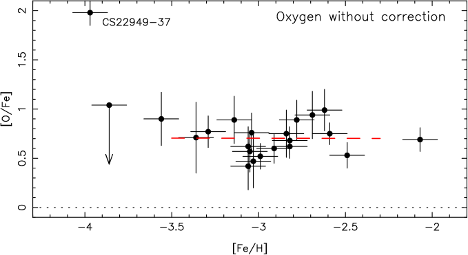
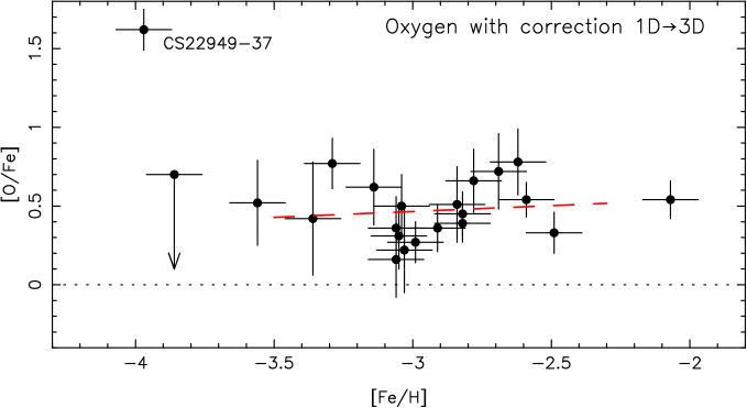
Figure 6: [O/Fe] plotted vs. [Fe/H], without and with a correction for stellar surface inhomogeneities (Nissen et al. NPA02 (2002)). The correction is uncertain since it has been computed for dwarfs. The slope of the regression line (dashed) is small and not significant.

The forbidden oxygen line is very weak, especially in the most metal-poor stars, where the line is generally below the limit of detection for [Fe/H] $<-3.5$. Hence, it has not been possible to determine oxygen abundances for all stars of the sample. However, the high quality of the spectra allowed a precise measurement to be made for most of our stars.

The oxygen line is located in a region where the S/N ratio of the spectra is the highest. Unfortunately, weak interference fringes from the CCD detector sometimes appear in this region and make the definition of the continuum more uncertain. We recall that the depression at the center of a 1mÅ line corresponds to only about 0.6% of the continuum, so the measurement of lines with an equivalent width below 1 mÅ is often difficult in this region of the spectrum. Moreover, in some unfortunate cases, the stellar oxygen line is superimposed on strong telluric lines in absorption or emission, and cannot be measured with sufficient precision, even after correction for night-sky emission or absorption lines (sky subtraction or division by the spectrum of a fast-rotating hot star).

We first computed the oxygen abundance using 1-D OSMARCS models. Plotting the [O/Fe] ratio as a function of [Fe/H] reveals no significant slope; the mean value is [O/Fe] $\approx 0.7$ (Fig. 6, upper panel). A large dispersion, on the order of 0.17 dex, is found.

Abundance corrections have been computed with 3-D radiative hydrodynamical codes by Nissen et al. (NPA02 (2002)) for metal-deficient dwarfs, but not for giant stars. However, they note that the sign of the correction is unlikely to change, and that therefore the [O/Fe] ratio based on [O I] lines should always be smaller in 3-D than in the 1-D computations. Thus, we assumed as a first approximation that the correction computed by Nissen et al. (NPA02 (2002)) is valid also for metal-deficient giants. The result of this exercise is shown in Fig. 6 (lower panel): The [O/Fe] still follows a “plateau,” which now lies at about [O/Fe] = 0.47.

Quite recently, Johansson et al. (JLL03 (2003)) have made a new determination of the $gf$ value for the Ni I 6300.34 line, itself actually a blend of ⁵⁸Ni and ⁶⁰Ni lines. This blend does not affect our own determinations of oxygen abundance, thanks to the smaller relative contribution of Ni to the blend in oxygen-enhanced stars. But it does affect our derived [O/Fe] values through a change of the solar oxygen abundance. Assuming that we are in the linear domain for line depths smaller than 5%, the new oscillator strength would increase the contribution of the Ni blend in the Sun from 29% to 43%, inducing a correction of $\log(57/71)\approx 0.1$ dex to the solar oxygen abundance and increasing our [O/Fe] values by the same amount. However, the superb fit obtained by Allende Prieto et al. (ALA01 (2001)), would likely also suffer from this significant enhancement of the Ni I contribution.

We finally note that the extremely metal-poor star CS 22949–037 has an exceptionally high O abundance according to Depagne et al. (DHS02 (2002)). It is, however, rather peculiar, displaying also very high abundances of Mg and several other elements, and should not be considered as representative of XMP stars in general. Indeed, the forbidden oxygen line is not detectable in any other star with [Fe/H]$\approx-4$ in our sample. If these stars have the same [O/Fe] ratio as the other XMP stars ([O/Fe] = 0.71 from 1-D models), then the computed equivalent widths of their [O I] lines would be less than 0.5m Å, a value which is generally below our detection limit.

Table 7: Coefficients of the adopted regression lines. In columns 2 and 3 are given the coefficients $a$ and $b$ of the relation [X/Fe] = $a$ [Fe/H] + $b$. In column 4 is given the scatter measured in the total interval, and in column 5 and 6 the scatter in two different intervals of metallicity. Column 7 lists an estimate of the scatter expected from measurement errors only. For some elements the total scatter is hardly larger than the expected error.

			$-4.1<$	$-4.1<$	$-3.1<$
			[Fe/H]	[Fe/H]	[Fe/H]
	Regression Line		$<-2.0$	$<-3.1$	$<-2.1$
	a	b	$\sigma_{\mathrm{reg}}$	$\sigma_{\mathrm{reg}}1$	$\sigma_{\mathrm{reg}}2$	$\sigma_{\mathrm{mes}}$
$\mathrm{Na}$	0.403$\pm$0.010	1.420$\pm$0.101	0.25	0.32	0.18	0.10
$\mathrm{Mg}$	0.035$\pm$0.003	0.380$\pm$0.029	0.13	0.11	0.15	0.09
$\mathrm{Al}$	0.047$\pm$0.005	-0.534$\pm$0.052	0.18	0.14	0.21	0.10
$\mathrm{Si}$	0.032$\pm$0.004	0.541$\pm$0.036	0.15	0.20	0.11	0.10
$\mathrm{K}$	0.176$\pm$0.002	1.020$\pm$0.023	0.11	0.13	0.10	0.10
$\mathrm{Ca}$	0.074$\pm$0.002	0.565$\pm$0.015	0.10	0.11	0.09	0.07
$\mathrm{Sc}$	0.034$\pm$0.002	0.178$\pm$0.019	0.11	0.14	0.08	0.07
$\mathrm{Ti}$	-0.014$\pm$0.001	0.185$\pm$0.013	0.09	0.09	0.10	0.05
$\mathrm{Cr}$	0.117$\pm$0.000	0.004$\pm$0.004	0.05	0.04	0.06	0.07
$\mathrm{Mn}$	0.030$\pm$0.003	-0.346$\pm$0.020	0.12	0.15	0.08	0.09
$\mathrm{Co}$	-0.131$\pm$0.002	-0.121$\pm$0.024	0.13	0.12	0.13	0.08
$\mathrm{Ni}$	-0.003$\pm$0.002	-0.048$\pm$0.020	0.11	0.13	0.11	0.09
$\mathrm{Zn}$	-0.271$\pm$0.002	-0.559$\pm$0.018	0.11	0.14	0.08	0.10

4.3 Light even-Z metals: Mg, Si, Ca, Ti

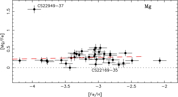
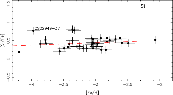
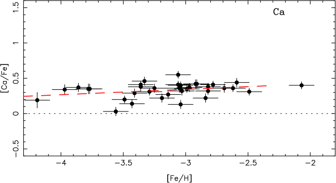
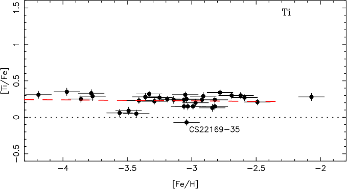
Figure 7: [Mg/Fe], [Si/Fe], [Ca/Fe] and [Ti/Fe] plotted vs. [Fe/H]. The peculiar star CS 22949–037 is not included in the computations of the scatter and of the regression line (dashed) for Mg. The star CS 22169–035 is deficient in all the light “even” elements.

In our spectra there are about 7 well-defined lines of magnesium, 15 lines of calcium, and about 30 lines of titanium, but silicon is represented by only two lines – one at 390.55 nm and the other at 410.29 nm. As the first line is severely blended by a CH line, we have chosen to use only the second one, which unfortunately falls in the wing of the H$\delta$ line. To compute the silicon abundances, synthetic profiles of the line were computed taking into account the presence of the H$\delta$ line.

Following A. Chieffi (private communication), Mg is formed during hydrostatic carbon burning in a shell and during explosive neon burning. Si and Ca are built during incomplete explosive silicon and oxygen burning, and Ti during complete and incomplete silicon burning. As shown in Fig. 7, they all appear to be enhanced relative to iron, but any slope with [Fe/H] is generally small (Table 7). The even-Z ($\alpha$) elements behave similarly to O, but the enhancement is smaller ([Mg/Fe] = +0.27, [Si/Fe] = +0.37, [Ca/Fe] = +0.33 and [Ti/Fe] = +0.23). The scatter around the mean value is small ($\sigma_{Mg}=0.13$ dex, $\sigma_{Si}=0.15$ dex, $\sigma_{Ca}=0.11$ dex, $\sigma_{Ti}=0.10$ dex); however, it increases slightly as the metallicity decreases. In Table 7 we list, for each element, the dispersion around the mean regression line in the intervals $\mathrm{[-4.1<[Fe/H]<-3.1]}$ and $\mathrm{[-3.1<[Fe/H]<-2.1]}$, as well as the value expected from measurement errors only.

The nearly identical abundance ratios of these light metals at low metallicity suggest that there is a similarly constant ratio between the yields of iron and of the other elements, in spite of the quite different sites where they are produced. In the case of magnesium, the spread around the mean value is not significantly larger than the measurement errors, even at the lowest metallicities. An exception is the peculiar star CS 22949–037, which is strongly enhanced in light elements (C, O, Na, Mg, Al) but has a “normal” abundance of Si, Ca, and Ti. This star is clearly an outlier and has not been taken into account in the computation of the “normal” trends and dispersions of the lighter elements.

4.4 The odd-Z metals: Na, Al, K, and Sc

4.4.1 NLTE effects

In extremely metal-deficient stars, the abundances of the odd-Z elements Na, Al, and K are deduced from resonance lines which are very sensitive to non-LTE effects. Hence, to determine the trends of these elements with metallicity it is important to take these effects into account, at least approximately.

The sodium abundance is computed from the Na D resonance lines at 589.0 nm and 589.6 nm. In some stars these lines are severely blended by interstellar lines, and the sodium abundance cannot be measured accurately. Baumüller et al. (BBG98 (1998)) have evaluated the importance of NLTE effects in metal-poor dwarfs and subgiants. They found that the correction can reach values as high as –0.5 dex. To account for this effect, the values of [Na/Fe] given in Tables 9 to 13 should thus be decreased by 0.5 dex.

The abundance of aluminium is based on the resonance doublet at 394.4 and 396.15 nm. Due to the high resolution and high S/N of the spectra, both lines can be used, and the blending of Al 394.4 nm by a CH line is easily taken into account. The Al abundance is underestimated in LTE computations (Baumüller & Gehren (BG97 (1997)); Norris et al. NRB01 (2001)), but since our stars are all very similar in temperature and gravity we can consider this correction to be similar and close to +0.65 dex for all the stars. As a consequence, the LTE abundance given in Tables 9 to 13 should be increased by about +0.65 dex.

The K abundance has been determined from the red doublet at 766.5 and 769.9 nm. Ivanova & Shimanskii (IS00 (2000)) have computed NLTE corrections for the K lines as a function of effective temperature and gravity. In the range $\mathrm{4}500<T_{eff}<5100$ K and $\mathrm{0.5<log\;g<2.0}$ the NLTE correction reaches $\sim-0.35$ dex. Thus, the LTE abundances given in Tables 9 to 13 should be decreased by about 0.35 dex (this correction has been taken into account in Fig. 9). Takeda et al. (T02 (1998)) propose NLTE corrections that are slightly smaller ($\sim-$0.25 dex), irrespective of metallicity or gravity.

We finally note that in the range of temperature, gravity, and metallicity covered by our sample we can assume that these corrections are similar for all the stars, thus they do not alter the general abundance ratio trends, only the levels of the relations.

4.4.2 The light elements Na and Al

The production of Na and Al is expected to be sensitive to neutron excess (Woosley & Weaver WW95 (1995)), and therefore depends on the amount of neutron-rich nuclei present in the supernova before the synthesis of these two odd-Z metals. Na is synthesized during hydrostatic carbon burning and partly in the hydrogen envelope (Ne, Na cycle), while Al is synthesized during carbon and neon burning and also in the hydrogen envelope (Mg, Al cycle).

In Fig. 8 we plot [Na/Fe] and [Al/Fe] vs. [Fe/H]. Both [Na/Fe] and [Al/Fe] exhibit a rather large scatter of $\sim$ 0.2 dex (Table 7). On the other hand, while Na decreases significantly with decreasing metallicity, Al remains practically constant within the range $\mathrm{-4.0<[Fe/H]<-3.0}$. The striking difference in the behavior of these two elements of very similar atomic numbers is puzzling, but there remains an alternative interpretation of the plot of [Na/Fe] vs. [Fe/H], which we consider in Sect. 5.2.

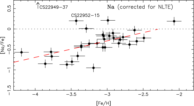
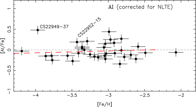
Figure 8: [Na/Fe] and [Al/Fe] plotted vs. [Fe/H]. The LTE abundances of these elements have been determined from resonance lines, but corrections for NLTE effects have been applied.

4.4.3 K and Sc

In this paper we present, for the first time, measurements of potassium abundances for a large sample of very metal-poor stars.

K is produced during explosive oxygen burning, while Sc is synthesized during explosive oxygen and neon burning. The Sc yields in the grid of Woosley & Weaver (WW95 (1995)) show large variations and thus appear to be strongly influenced by the parameterisation of the explosion (Samland Sam98 (1998)). The Sc yields also show very large variations as a function of the mass of the progenitor in the computations of Chieffi & Limongi (CL02 (2002)); thus we might expect a large scatter of the ratio [Sc/Fe] vs. [Fe/H].

In Fig. 9 the ratios [K/Fe] and [Sc/Fe] have been plotted vs. [Fe/H]; they seem to decrease slowly with metallicity with a moderate scatter (about 0.12 dex), although the slope is not very significant (Table 7). The star CS 30325–094 appears to be K- and Sc-rich, while the more metal-poor star CS 22885–096 is rich in Sc, with a “normal” K abundance.

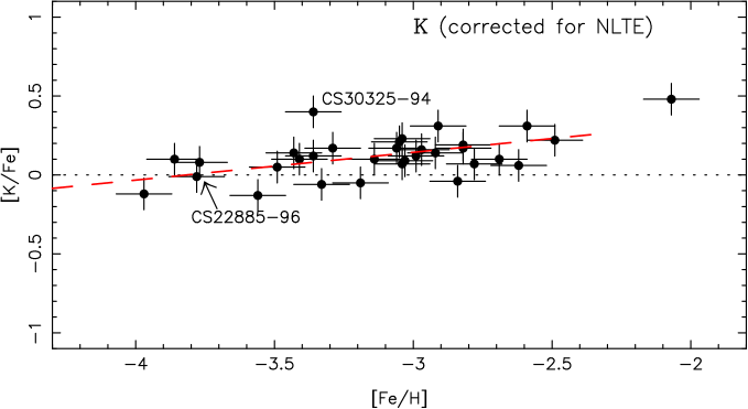
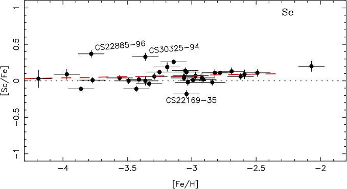
Figure 9: [K/Fe] and [Sc/Fe] plotted vs. [Fe/H]. An NLTE correction has been applied to our potassium abundance measurements (see text).

4.5 Iron-peak elements

Generally speaking, the iron-peak elements are built during supernova explosions. More specifically, Cr, Mn, Fe, Co, Ni, and Zn are built during (complete or incomplete) explosive silicon burning in two different regions characterized by the peak temperature of the shocked material (Woosley & Weaver WW95 (1995); Arnett Arn96 (1996); Chieffi & Limongi CL02 (2002); Umeda & Nomoto UN02 (2002)).

4.5.1 Cr and Mn

Six manganese lines are visible in our spectra but three of them belong to the resonance triplet ($a^{6}S-z^{6}P^{0}$). The abundance of Mn deduced from this triplet is systematically lower (–0.4 dex) than the abundance deduced from the other manganese lines, and thus has not been taken into account in the mean. (The difference can be due to NLTE effects or to a bad estimation of the gf values of the lines of this multiplet). However, for the five most metal-poor stars only the resonance triplet was detected. In this case the abundance deduced from these lines has been systematically corrected by 0.4 dex (and are the values given in Tables 9 to 14).

Cr and Mn are produced mainly by incomplete explosive silicon burning (WW95 (1995); Chieffi & Limongi CL02 (2002); Umeda & Nomoto UN02 (2002)). The observed abundances of these elements have previously been shown to decrease with decreasing metallicity (McWilliam et al. MPS95 (1995); Ryan et al. RNB96 (1996); Carretta et al. CGC02 (2002)).

As shown in Fig. 10, the slope of [Cr/Fe] vs. [Fe/H] is smaller than that found by Carretta et al. (CGC02 (2002)). Moreover, our precise measurements show that [Cr/Fe] exhibits extremely small scatter ($\sigma=0.05$ dex over the entire metallicity range; see Table 7). This scatter is no larger than expected from measurement errors alone, indicating that any intrinsic scatter is extremely small and that the production of Fe and Cr are very closely linked. Among all elements measured in extremely metal poor stars, no other element follows iron so closely. We discuss this point further in section 5.3).

Present nucleosynthesis theories do not yet provide a clear explanation for this close link between Fe and Cr, together with the observed decrease of [Cr/Fe] with decreasing metallicity. This is even more puzzling since the metallicity ([Fe/H]) of a given XMP star may be considered as the ratio of the iron yield to the volume of H gas swept up by the ejecta, which is a priori independent of the nucleosynthesis which takes place in the exploding SN and drives the [Cr/Fe] ratio. However, as argued by Ryan et al. (RNB96 (1996)) and explored further by Umeda & Nomoto (UN02 (2002)), both the amounts of gas swept up and the supernova yields may be correlated through the energy of the explosion, which depends in turn on the mass of the progenitor. But the low scatter is surprising.

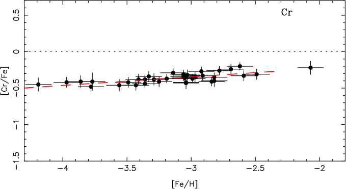
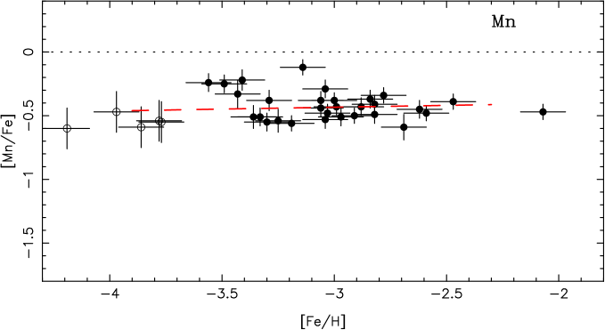
Figure 10: [Cr/Fe] and [Mn/Fe] plotted vs. [Fe/H]. For Mn the hyperfine structure has been taken into account, and only the lines with an excitation potential larger than 2.2 have been used. When these lines are too weak (open symbols) the abundance has been deduced from the resonance lines and corrected.

The relation [Cr/Mn] vs. [Fe/H] shows practically no trend with metallicity in the range $\mathrm{-4.0<[Fe/H]<-2.5}$ (Fig. 11). However at low metallicity the manganese abundance is deduced from the resonance lines and a correction of 0.4 dex is empirically applied. An NLTE 3D analysis of these lines would be necessary to be sure that no significant slope is found, but it seems that the ratio Cr/Mn is close to the solar value in the most metal-poor stars, although Mn is an odd-Z element and Cr an even-Z element.

Figure 11: [Cr/Mn] plotted vs. [Fe/H]. The symbols are the same as in Fig. 10. The ratio Cr/Mn is almost constant and close to the solar value.

4.5.2 Co, Ni, and Zn

Fe, Co, Ni, and Zn are produced mainly in complete explosive Si burning. The abundance trends of these elements are presented in Fig. 12.

McWilliam et al. (MPS95 (1995)) found that [Co/Fe] increases with decreasing [Fe/H]. We confirm this trend (Fig. 12), but the slope of the relation we obtain ($\sim 0.13$ dex per dex) is not as steep as they found. Also, the scatter in our data ($\approx 0.15$ dex) is significantly larger than expected from measurement errors alone.

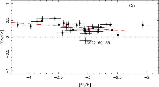
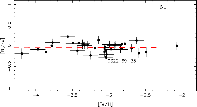
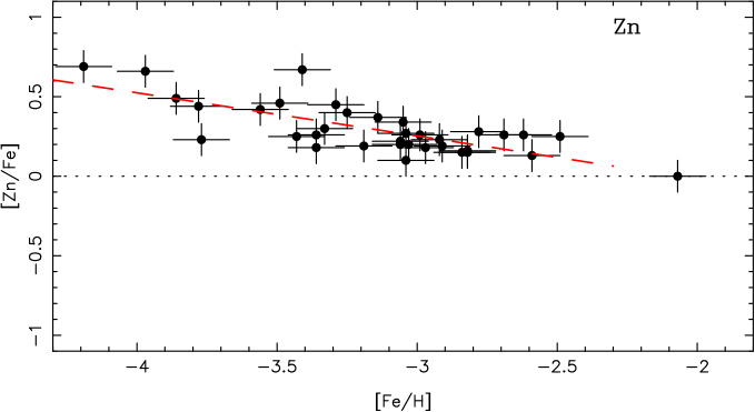
Figure 12: [Co/Fe], [Ni/Fe], and [Zn/Fe] plotted vs. [Fe/H]. These ratios increase ([Co/Fe], [Zn/Fe]) or remain essentially constant ([Ni/Fe]) with decreasing metallicity.

Co and Ni are thought to be synthesized in the same nuclear process, but unlike [Co/Fe], [Ni/Fe] shows a mean value close to zero and no trend with [Fe/H]. The yields of Ni and Fe have a constant ratio, but the correlation is not as tight as that between Cr and Fe. Three stars, CS 22189–009, CS 22885–096 and CS 22897–008, had been previously claimed to be Ni-rich by McWilliam et al. ([Ni/Fe]$>+0.75$). These stars are included in our sample, but are found to have a normal Ni abundances. In our computations we have rejected the line at 423 nm for which no $gf$ value has been measured. The “solar $gf$ value” computed by McWilliam et al. results in a Ni abundance from this line which systematically disagrees with the value found from the other three lines.

Zinc is an interesting element, as it is produced by complete silicon burning, but it has been suggested that it could also be formed by slow or rapid neutron capture (Heger & Woosley HW02 (2002); Umeda & Nomoto UN02 (2002)). If Zn were formed by the $s$-process, we would expect that [Zn/Fe] would decrease with metallicity, at variance with what we observe. On the other hand, in CS 31082–001, a star with [Fe/H] = –3.0 and extremely rich in $r$-process elements, Hill et al. (HPC02 (2002)) found the Zn abundance to be normal relative to other stars with [Fe/H] = –3.0). We conclude that neither the $s$-process nor the $r$-process in their progenitors appears likely to have contributed a significant fraction of the Zn in these stars.

The ratio [Zn/Fe] increases with decreasing [Fe/H] more clearly than does [Co/Fe], in agreement with the results by Primas et al. (2000). The increase is quite significant and seems to be the signature of an $\alpha$-rich freeze-out process.

We recall that the abundances in the peculiar star CS 22949–037 were found by Depagne et al. (DHS02 (2002)) to correspond to the expected yields (Woosley & Heger, private communication) of a rather massive progenitor ($\mathrm{M=35M_{\sun}}$), assuming a high mass cut some mixing and a rather large fallback (due to the large mass of the central remnant). The [Zn/Fe] ratio of this star is, however, similar to the “normal” stars of the sample and seems to be a global feature of extremely metal-poor stars.

5 Discussion

Figure 13: Abundance ratios [X/Mg] plotted vs. [Mg/H]. The scale is the same for all the plots: the amplitude in the coordinate [X/Mg] is 2.2 dex. For Mn the symbols are the same as in Fig. 10

5.1 Comparison with previous studies of very metal-poor stars

The trends of the relations [X/Fe] vs. [Fe/H] reported in the present study are generally in agreement with previous results in the literature, such as those of McWilliam et al. (MPS95 (1995)), Ryan et al. (RNB96 (1996)), and Norris, Ryan, & Beers (NRB01 (2001)). However, the much smaller scatter of the ratios [X/Fe] is a notable result of the greatly improved spectra obtained for this study.

Carretta et al. (CGC02 (2002)) observed three very metal-poor MS or TO stars and two extremely metal-poor giants ([Fe/H] $<-3.0$) with Keck spectra having a figure of merit F (Norris et al. NRB01 (2001)) larger than 600. The elements from Mg to Fe were analyzed. Within a (rather large) scatter the two analyses are compatible, except for a few elements, in particular Cr (their slope of [Cr/Fe] vs. [Fe/H] seems to be steeper than ours).

5.2 Mg as an alternative “reference element”

Iron is a convenient “reference element” in high-resolution spectral analyses, because it has by far the largest number of usable lines and is represented by two ionization states. Iron may not be the best choice as a tracer of Galactic chemical evolution, however, since its nucleosynthesis channels are not very well understood, and are not necessarily even unique (e.g., explosive nucleosynthesis, Si burning in massive SNe II, or SNe Ia).

From the point of view of the chemical evolution of the Galaxy oxygen would be a better choice (see Wheeler, Sneden & Truran WST89 (1989)), as oxygen is the most abundant element after H and He, it comes from a single source, and its abundance should not be significantly affected in the explosive phase. However, its well-known observational difficulties would considerably degrade the accuracy of the derived trends: Oxygen could be measured in only 21 of our programme stars and the uncertainties on its abundance are large (see in particular Sect. 3.3 and the error bars in Fig. 6).

Mg or Ca might be good alternatives. The abundances of these elements are accurately determined, and they are also formed mainly in massive SNe. We choose Mg rather than Ca here (Fig. 13), because Mg is more robust in the sense that its production is dominated by hydrostatic burning processes and it is also less affected by explosive burning and by “fallback” (Woosley & Weaver WW95 (1995)). Note that Shigeyama & Tsujimoto (ST98 (1998)) also recommended Mg rather than Fe as a useful reference element, following much the same logic. We note, however, that the “plateau”-like behavior of [Mg/Fe] with increasing iron abundance in the range $-$4 to $-$2 implies that Mg and Fe have parallel early nucleosynthesis histories. Therefore, the trends of elemental ratios with [Fe/H] found in section 4 should survive if [Fe/H] is replaced by [Mg/H] as a metallicity indicator.

Yet, the new diagrams (see Fig. 13) present a few notable differences. One is expected – the scatter is never as low as in some of the earlier diagrams because [Mg/H] is determined less accurately than [Fe/H], being based on 8 lines instead of 150. The other – new – result is very interesting: rather than a roughly linear variation over the full range $-4.0<$ [Mg/H] $<-2.5$, there is a hint that all abundance ratios are flat in the interval $-4.0<$ [Mg/H] $<-3.0$, with something qualitatively different occurring at higher metallicity.

This pattern is in fact what is expected if the first SNe are primordial and have specific yields: the plateau between $-4.0$ and $-3.0$ would then reflect a pure zero-metallicity type of SNe, whereas at higher metallicity we may observe a mix of primordial and non-primordial SNe. At still higher metallicities ($\geq$ –2.0), the scatter is expected to decrease again because so many SN precursors are involved that any differences average out.

We now consider a few elements of particular interest.

$\bullet$ Carbon
Karlsson & Gustafsson (KG01 (2001)) have statistically simulated the chemical enrichment of a metal-poor system, assuming that the stellar yields are one-dimensional functions of the progenitor mass of the supernovae and the masses of the supernovae are distributed according to a Salpeter IMF. In particular, they computed the distribution of the abundance ratio [C/Mg] vs. [Mg/H] in a hypothesized sample of 500 XMP stars (their Fig. 3), adopting the yields of either Woosley & Weaver (WW95 (1995)) or Nomoto et al. (NHT97 (1997)). Our Fig. 13 for C is compatible with their Fig. 3a (yields of Woosley & Weaver), but not with their Fig. 3b (yields of Nomoto et al.).

On the other hand, both in their simulation and as observed in our present sample, the [C/Mg] ratio seems to decrease with increasing [Mg/H]. Following Karlsson and Gustafsson (KG01 (2001)), this effect could be the result of different supernova masses operating at different metallicities. SNe producing a high [C/Mg] ratio produce only small amounts of Mg; on the contrary, SNe producing a low [C/Mg] ratio also produce substantial Mg.

Karlsson & Gustafsson show that the patterns they predict become barely visible (or invisible) in an observational sample smaller than N $\approx 500$ and affected by uncertainties of the order of 0.1 dex. We have examined how their [C/Mg] vs. [Mg/Fe] diagram would appear for our sample (Fig. 14). Not only is no fine structure visible, but our diagram is considerably more extended in the vertical direction, strongly suggesting that the scatter in [C/Mg] is not explained by the theoretical yields.

Figure 14: [C/Mg] vs. [Mg/Fe] for all stars of our sample with temperatures higher than 4800 K (and thus presumably not mixed). Filled circles represent the most metal-poor stars ([Fe/H] $\leq-3.0$), open circles the stars with [Fe/H]$>-3.0$. The variation of [C/Mg] is larger than expected from the computations of Karlsson & Gustafsson (KG01 (2001)), suggesting that the scatter in [C/Mg] is not explained by the theoretical yields.

$\bullet$ Sodium and Aluminium
[Na/Fe] and [Al/Fe] exhibit very different behaviours as functions of [Fe/H] (Fig. 8). However, when Mg is used as a reference element (Fig. 13), the behavior of these elements appears rather similar, and a plateau at the lowest metallicities appears for Na as well as for Al: below $\mathrm{[Mg/H]=-3.0}$, [Na/Mg] remains constant at about [Na/Mg] = 0.9 (in fact this plateau appears also in Fig. 8: [Na/Fe] $\approx 0.7$ for [Fe/H]$<-3.4$). However, the rise in [Na/Mg] at higher metallicity is not seen for Al.

The discrepant position of CS 22952–015 in the diagrams of [Na/Mg] and [Al/Mg] vs. [Mg/H] will be discussed in Sect. 5.5.

$\bullet$ Iron peak elements
There is no clear slope of [Cr/Mg] vs. [Mg/H], as was seen for [Cr/Fe] vs. [Fe/H]. This raises the suspicion that the slope in the latter diagram may be an artifact due to different NLTE corrections for the two elements as a function of metallicity (Thévenin & Idiart TI99 (1998)). These corrections have not been applied, as they are not known for Cr and have not been published line by line for Fe. We return to this question below.

No significant slope is found for [Mn/Mg], (in agreement with absence of slope for [Mn/Fe]). Similarly, for [Mg/H]$<-3.0$ no clearly significant slope is found for the other elements (Fe, Co, Ni, Zn) .

5.3 Cosmic vs. observational scatter in the abundance ratios

A key motivation for the present programme was to explore to what extent the scatter in the observed abundance ratios is due to observational error, and to what extent it reflects physical conditions in the early Galaxy when these stars were formed. McWilliam et al. (MPS95 (1995)) and McWilliam & Searle (MS99 (1999)) already noted that the scatter in some of their diagrams of [X/Fe] vs. [Fe/H] could be entirely accounted for by observational errors. The issue was summarized by Ryan, Norris, & Beers (RNB96 (1996)) as follows. “The abundance patterns, especially those of Cr, Mn, or Co, raise the following question: why should all halo supernova ejecta around this epoch that possess a particular [Cr/Fe] ratio (or [Mn/Fe] ratio or [Co/Fe] ratio) subsequently form into stars of the same [Fe/H]? Put differently, how do the ejecta know how much interstellar hydrogen to combine with?”.

Our observations were designed to achieve twice the spectral resolution and 3–4 times the S/N ratio of the earlier data in order to test this very point. With our much lower observational errors, we can conclude that while the scatter for C, Na, Mg, Al, and Si is probably real, the very small scatter of Ca, Cr, and Ni still do not leave room for the existence of an intrinsic scatter!

Consider the case of chromium, which has the lowest observed scatter (r.m.s. 0.05 dex). The problem mentioned earlier is very acute and derives from the simultaneous absence of scatter and presence of of a slope of [Cr/Fe] versus metallicity. Although one can argue that the amount of hydrogen swept up by the ejecta is mainly determined by the energy of the explosion of the SN (Cioffi et al. CMB88 (1988)), thus relating the abundance ratios produced by the SN to the final [Fe/H] of the enriched gas, it is still difficult to believe that there is so little room for noise in the mixing process. However, if the slope is in fact spurious (e.g., due to neglected differential NLTE corrections between Cr and Fe), as suggested by the diagram of [Cr/Mg] vs. [Mg/H] (Fig. 13), the problem vanishes. One would simply conclude that Cr and Fe are produced together, independent of the metallicity of the SN progenitor, and the amount of mixing cannot be localized anymore along the metallicity axis. Until detailed NLTE computations for Cr and Fe become available we cannot decide if this interpretation is correct.

For all the elements discussed here, our results show that the scatter of their production ratios is very small, far below the values derived earlier. This implies that we are observing either the ejecta of fairly large bursts of massive stars, so the sampling of the IMF is reasonably good, or the result of several events promptly mixed by strong turbulence.

5.4 The nature of the first supernovae

Theoretical work (Bromm et al. BFC01 (2001) and references therein) predict that the first stellar generation is made of very massive stars, with masses above 100 M_⊙, because zero-metal matter lacks adequate cooling mechanisms for fragmenting down to classical supernova-progenitor masses. Results of WMAP (Kogut et al. KSB03 (2003)) on an early reionization of the Universe have triggered further claims (Cen Cen03 (2003)) of a very massive stellar generation.This has very important implications for early ’stellar’ nucleosynthesis. According to current models, such stars either end up as pair-instability supernovae, or as collapsed black holes, in the latter case with no contribution to the metal enrichment of the ISM (Heger & Woosley HW02 (2002); Umeda & Nomoto UN02 (2002)). A comparison of the yields of Heger & Woosley with our results show a clear disagreement, in particular the predicted strong odd-even effect, not seen in our observations, and a strong decline of Zn with metallicity also not observed. Nakamura et al. (NUI01 (2001)) and Nomoto et al. (NHT97 (1997)) have computed yields of SNe with a progenitor mass of 25 M_⊙ of very high energy (also called hypernovae). Their predicted yields have some positive features at very low metallicity, such as the high [Zn/Fe] and [Co/Fe], and a low [Mn/Fe], as observed. However they also predict a lack of [O/Fe] enhancement, in clear disagreement with our observations.

Our conclusion is that classical SNe are still the best candidates to explain our observational results.

5.5 Peculiar objects

5.5.1 CS 22949–037

The highly peculiar abundances of CS 22949–037 were studied in detail by Depagne et al. (DHS02 (2002)). They may be explained by a single progenitor or by an enrichment event dominated by massive SNe II with substantial fallback; this applies also to the similar star CS 29498–043 analysed by Aoki et al. (2002a , 2002b ).

Tsujimoto & Shigeyama (TS03 (2003)) propose another interpretation of CS 22949–037 and CS 29498–043. The high [Mg/Fe] ratio could be due to a low-energy explosion, strong enough to eject the layers containing the light elements, but ejecting little iron and other iron-peak elements. In this interpretation, the lack of Fe relative to the lighter elements O and Mg is also associated with a large fallback on the remnant, but due to a low explosion energy rather than a large mass of the collapsed core as in the model adopted by Depagne et al. (DHS02 (2002)). However, the normal Cr/Mn/Fe/C/Ni ratios observed in this star would rather suggest a normal explosion energy, the larger fallback being due to a larger mass of the single or multiple progenitors.

Further exploration of the precise abundance patterns of these two putative low-energy supernova descendents should be quite interesting. This interpretation would link the exceptional cases of the most extreme metal-poor stars with rather low-mass progenitors. It would, however, conflict with the usual interpretation which associate the more massive progenitors with both the earliest explosions and the largest volume of hydrogen swept up, resulting in low metallicity in the ISM. The problem clearly requires further investigation.

5.5.2 CS 22952–015

CS 22952–015 is known to be Mg deficient (McWilliam et al., MPS95 (1995)). In the abundance ratio plots vs. [Mg/H] (Fig. 13), it does indeed appear Fe-rich, but its most notable characteristic is the large values of [Na/Mg] and [Al/Mg]. An interesting point is that this effect is not seen as clearly in the diagrams of [Na/Fe] and [Al/Fe] vs. [Fe/H] (Fig. 8), because all three elements Na, Al, and Fe are enhanced relative to Mg in CS 22952–015.

5.5.3 CS 22169–035

CS 22169–035 appears to be particularly deficient in Ti (Fig. 7), but in fact all the ratios [Mg/Fe], [Si/Fe], [Ca/Fe], [Co/Fe], [Ni/Fe], and [Zn/Fe] are low as well. When Mg is used as the reference element, this star has a normal position in the diagrams, and the abundance anomalies are most simply characterised as a deficiency of Fe.

5.6 Yields of the first supernovae

With Mg chosen as the reference element (Fig. 13), the most metal-poor stars in our sample ([X/H]$<-2.9$) define a plateau at abundance ratios [X/Mg] corresponding to the yields of the first supernovae, thus providing constraints on these yields. The mean value of [X/Mg] of each plateau is given in Table 8 and represent our best estimate of the yields from the first metal producers in the Galaxy.

Table 8: Mean [X/Mg] ratios for stars with [Mg/H]$<-2.9$, corresponding to the yields of the first supernovae. The r.m.s. is the scatter around the mean.

		$r.m.s.$	n
$[$Na/Mg]	$-$0.84	0.22	11
$[$Al/Mg]	$-$0.33	0.15	13
$[$Si/Mg]	$+$0.21	0.14	14
$[$K/Mg]	$-$0.14	0.14	13
$[$Ca/Mg]	$+$0.06	0.09	14
$[$Sc/Mg]	$-$0.17	0.14	14
$[$Ti/Mg]	$-$0.01	0.09	14
$[$Cr/Mg]	$-$0.63	0.09	14
$[$Mn/Mg]	$-$0.65	0.20	14
$[$Fe/Mg]	$-$0.21	0.10	14
$[$Co/Mg]	$+$0.13	0.17	14
$[$Ni/Mg]	$-$0.23	0.13	14
$[$Zn/Mg]	$+$0.15	0.19	14

In Fig. 15a, these mean values are compared to the values predicted by Woosley & Weaver (WW95 (1995)) for their zero-metal supernova models 15A, 25B and 35C (progenitor masses 15, 25 and 35 $M_{\odot}$). The Woosley & Weaver values of [X/Mg] for the elements from C to Ca have been enhanced in order to bring their predicted value of [Fe/Mg] into agreement with our observations.

In Fig. 15b we compare with the zero-metal models of Chieffi & Limongi (CL03 (2003)) for 15, 20, 35, 50 $M_{\odot}$ stars. The predicted [X/Mg] values were already adjusted by Chieffi & Limongi to obtain [Mg/Fe]$\approx+0.45$). These comparisons suggest that some adjustment of the models is indeed required.

The connection between the abundances observed in these very old stars and those observed in intergalactic clouds – in particular the damped Ly_α systems (DLA) – will be further discussed in subsequent papers.

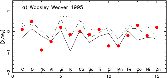
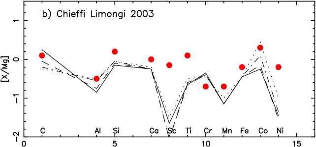
Figure 15: Mean [X/Mg] values for [Mg/H]$<-3$ (Fig. 7 and Table 8) compared to the model yields by: a) Woosley and Weaver for 15 (dotted line), 25 (dashed), and 35 $M_{\odot}$ SNe (full), and b) Limongi and Chieffi for 15 (dotted line), 20 (dotted-dashed), 35 (dashed), and 50 $M_{\odot}$ (full).

6 Conclusions

We have studied the abundances of 17 elements from C to Zn in a sample of 35 halo giant stars in the metallicity range –4.0 $<$ [Fe/H] $<$ –2.7. Our VLT/UVES spectra have resolving power $R=47,000$ and S/N ratio per pixel between 100 and 200 – far better than former data obtained with 4-m class telescopes. The lowest possible metallicity range was chosen because, according to previous theoretical work, this is where one expects to see the imprint of SN ejecta from either single SNe or single bursts of star formation.

$\bullet$ We have shown that in very metal-poor giants the continuous opacity in the UV is dominated by the Rayleigh scattering, and it is therefore crucial in this region to properly account for continuum scattering, as it has been done in this work. (A still better approach would be to take also scattering into account in the line formation).

$\bullet$ Our first and probaby most important conclusion is the existence of a surprisingly well-defined pattern of abundance ratios, with a cosmic scatter often at (or below) the level of detection (with the exception of carbon). Given the exceptional quality of our observations, our upper limit to the cosmic scatter is 3-4 times lower than former determinations.

$\bullet$ Trends with metallicity, visible as mild slopes in diagrams of [X/Fe] vs. [Fe/H] (X being any element between Na and Zn), tend to disappear when [X/Mg] vs. [Mg/H] are chosen as the diagnostic diagrams (at least when [Mg/H] $\leq-3.0$). At the lowest [Mg/H], practically no slope is present, suggesting that the level of “primordial yields” may have been reached.

$\bullet$ In the diagram [Cr/Fe] vs. [Fe/H] the intrinsic scatter is so small as to raise the suspicion that the mild slope might be due to residual, metallicity-dependent, differential NLTE corrections to our abundances for Cr and Fe, rather than to a variation of the [Cr/Fe] ratio in the yields. The lack of any slope when Mg is taken as the reference element supports this hypothesis. Moreover, if there were real changes in the [Cr/Fe] ratio in the yields, we would have to explain how the ejecta could be diluted in the environment without producing significant scatter in [Cr/Fe] at given [Fe/H], a rather unlikely scenario. Our result for [Cr/Fe] makes clear that progress on the interpretation of our observational data requires further progress in stellar atmosphere theory. NLTE computations are available for only a few elements, and 3-D effects have not yet been computed for giants – a special concern for our sample, which consists exclusively of giants.

$\bullet$ The low scatter in our observed abundance ratios suggests that they are the results of enrichment events that are not single SNe (we should then see scatter due to the different masses of each SN), but rather of single “burst” events.

$\bullet$ Our results are clearly incompatible with the predicted yields of pair-instability supernovae/hypernovae (Umeda & Nomoto UN02 (2002), Heger & Woosley HW02 (2002)). Neither the expected strong odd-even effect nor the predicted Zn deficiency is observed. Very high-energy SNe, with explosive energies of the order of $10^{53}$ ergs, are not good candidates either, as they under-produce oxygen (Nakamura et al. NUN99 (1999)). Only when mixing and fallback are added is a better fit obtained (Umeda & Nomoto UN02 (2002)).

$\bullet$ A detailed comparison of our observations with theoretical supernova yields is deferred to a forthcoming paper. However, a first comparison has been made with standard sources of theoretical yields of SNe with progenitor masses in the usual range from 12 to 70 $M_{\sun}$. While not perfect, they still give the best available fit, at least when compared to more exotic processes. This has implications for the kinds of massive stars that are thought to have reionized the Universe as early as 200 million years after the Big Bang, according to the recent results from WMAP.

Our abundance results for elements heavier than Zn (e.g., Sr, Ba, etc.) and detailed comparisons with Galactic chemical evolution models will be discussed in forthcoming papers.

Table 9: Abundances of the elements in the selected stars. Na Al and K are NOT corrected for non-LTE effects and O is computed with 1D models

HD 2796    [Fe/H]=–2.47
	$log\varepsilon$	[M/H]	[M/Fe]	$\sigma$	N
C	5.55	-2.97	-0.51	-	-
N	-	-	-	-	-
O	6.80	-1.97	0.50	-	-
Na	4.20	-2.13	0.34	-	2
Mg	5.36	-2.22	0.25	0.14	7
Al	3.35	-3.12	-0.66	-	2
Si	5.48	-2.07	0.40	-	1
K	3.25	-1.87	0.60	-	2
Ca	4.22	-2.14	0.32	0.10	16
Sc	0.79	-2.38	0.09	0.11	7
Ti I	2.75	-2.27	0.20	0.06	12
Ti II	2.79	-2.23	0.24	0.09	28
Cr	2.95	-2.72	-0.26	0.13	7
Mn	2.54	-2.85	-0.39	0.01	3
Fe I	5.05	-2.45	0.01	0.13	114
Fe II	5.02	-2.48	-0.02	0.13	17
Co	2.59	-2.33	0.14	0.08	2
Ni	3.70	-2.55	-0.09	0.14	3
Zn	2.37	-2.23	0.24	-	1

HD 122563    [Fe/H]=–2.82
	$log\varepsilon$	[M/H]	[M/Fe]	$\sigma$	N
C	5.30	-3.22	-0.41	-	-
N	-	-	-	-	-
O	6.57	-2.20	0.62	-	-
Na	3.75	-2.58	0.23	-	2
Mg	5.13	-2.45	0.36	0.12	8
Al	3.28	-3.19	-0.38	-	2
Si	5.20	-2.35	0.47	-	1
K	2.82	-2.30	0.51	-	1
Ca	3.86	-2.50	0.31	0.10	16
Sc	0.46	-2.71	0.11	0.10	7
Ti I	2.32	-2.70	0.12	0.10	14
Ti II	2.38	-2.64	0.18	0.10	28
Cr	2.46	-3.21	-0.40	0.17	7
Mn	2.17	-3.22	-0.41	0.06	3
Fe I	4.72	-2.78	0.03	0.17	142
Fe II	4.65	-2.85	-0.04	0.13	18
Co	2.39	-2.53	0.29	0.13	4
Ni	3.47	-2.78	0.03	0.09	3
Zn	1.94	-2.66	0.16	-	2

HD 186478    [Fe/H]=–2.59
	$log\varepsilon$	[M/H]	[M/Fe]	$\sigma$	N
C	5.60	-2.92	-0.34	-	-
N	5.75	-2.17	0.42	-	-
O	6.93	-1.84	0.75	-	-
Na	3.94	-2.39	0.20	-	2
Mg	5.38	-2.20	0.39	0.08	7
Al	3.32	-3.15	-0.57	-	2
Si	5.40	-2.15	0.44	-	1
K	3.19	-1.93	0.66	-	2
Ca	4.21	-2.15	0.44	0.10	16
Sc	0.68	-2.49	0.10	0.12	7
Ti I	2.68	-2.34	0.25	0.07	13
Ti II	2.72	-2.30	0.29	0.10	26
Cr	2.76	-2.91	-0.33	0.14	7
Mn	2.33	-3.06	-0.48	0.04	3
Fe I	4.93	-2.57	0.01	0.18	140
Fe II	4.90	-2.60	-0.01	0.14	18
Co	2.54	-2.38	0.21	0.19	4
Ni	3.49	-2.76	-0.18	0.15	3
Zn	2.14	-2.46	0.13	-	1

BD+17:3248    [Fe/H]=–2.07
	$log\varepsilon$	[M/H]	[M/Fe]	$\sigma$	N
C	6.02	-2.50	-0.44	-	-
N	6.42	-1.50	0.57	-	-
O	7.39	-1.38	0.69	-	-
Na	4.95	-1.38	0.69	-	2
Mg	5.70	-1.88	0.19	0.10	7
Al	3.70	-2.77	-0.71	-	2
Si	6.00	-1.55	0.52	-	2
K	3.88	-1.24	0.82	-	2
Ca	4.69	-1.67	0.40	0.08	14
Sc	1.30	-1.87	0.20	0.16	6
Ti I	3.18	-1.84	0.23	0.08	12
Ti II	3.28	-1.74	0.33	0.17	29
Cr	3.39	-2.28	-0.22	0.20	6
Mn	2.86	-2.53	-0.47	0.02	3
Fe I	5.46	-2.04	0.02	0.15	141
Fe II	5.41	-2.09	-0.03	0.09	16
Co	3.21	-1.71	0.36	-	2
Ni	4.19	-2.06	0.00	0.08	3
Zn	2.54	-2.06	0.00	-	1

BD-18:5550    [Fe/H]=–3.06
	$log\varepsilon$	[M/H]	[M/Fe]	$\sigma$	N
C	5.44	-3.08	-0.02	-	-
N	-	-	-	-	-
O	6.13	-2.64	0.42	-	-
Na	3.32	-3.01	0.05	-	2
Mg	4.83	-2.75	0.31	0.15	8
Al	2.82	-3.65	-0.59	-	2
Si	4.88	-2.67	0.39	-	1
K	2.58	-2.54	0.52	-	2
Ca	3.71	-2.65	0.41	0.10	16
Sc	0.15	-3.02	0.04	0.09	7
Ti I	2.12	-2.90	0.16	0.04	13
Ti II	2.10	-2.92	0.14	0.09	30
Cr	2.27	-3.40	-0.34	0.10	7
Mn	1.95	-3.44	-0.38	0.05	3
Fe I	4.44	-3.06	0.00	0.12	148
Fe II	4.44	-3.06	0.00	0.10	17
Co	2.05	-2.87	0.19	0.12	3
Ni	3.14	-3.11	-0.05	0.10	3
Zn	1.76	-2.84	0.22	-	1

CD-38:245    [Fe/H]=–4.19
	$log\varepsilon$	[M/H]	[M/Fe]	$\sigma$	N
C	$<$4.00	$<$-4.52	$<$-0.33	-	-
N	-	-	-	-	-
O	-	-	-	-	-
Na	2.08	-4.25	-0.06	-	2
Mg	3.59	-3.99	0.20	0.08	6
Al	1.61	-4.86	-0.67	-	2
Si	3.56	-3.99	0.20	-	1
K	-	-	-	-	-
Ca	2.37	-3.99	0.20	0.17	8
Sc	-0.98	-4.15	0.04	-	2
Ti I	1.20	-3.82	0.37	0.04	5
Ti II	1.08	-3.94	0.25	0.11	24
Cr	1.04	-4.63	-0.44	0.12	5
Mn	0.61	-4.78	-0.60	0.03	3
Fe I	3.30	-4.20	-0.01	0.20	95
Fe II	3.33	-4.17	0.02	0.13	7
Co	1.10	-3.82	0.37	0.08	3
Ni	1.88	-4.37	-0.19	-	2
Zn	1.10	-3.50	0.69	-	1

Table 10: Abundances of the elements in the selected stars. Na Al and K are NOT corrected for non-LTE effects and O is computed with 1D models

BS 16467–062    [Fe/H]=–3.77
	$log\varepsilon$	[M/H]	[M/Fe]	$\sigma$	N
C	5.00	-3.52	0.25	-	-
N	-	-	-	-	-
O	-	-	-	-	-
Na	2.39	-3.94	-0.17	-	2
Mg	3.97	-3.61	0.16	0.09	7
Al	1.80	-4.67	-0.90	-	2
Si	4.20	-3.35	0.42	-	1
K	1.78	-3.34	0.43	-	2
Ca	2.94	-3.42	0.35	0.19	12
Sc	-0.59	-3.76	0.01	0.06	4
Ti I	1.65	-3.37	0.40	0.17	11
Ti II	1.43	-3.59	0.18	0.18	23
Cr	1.49	-4.18	-0.41	0.29	5
Mn	1.07	-4.32	-0.55	0.03	3
Fe I	3.67	-3.83	-0.06	0.14	130
Fe II	3.79	-3.71	0.06	0.12	4
Co	1.70	-3.22	0.55	0.10	4
Ni	2.56	-3.69	0.08	0.03	3
Zn	1.06	-3.54	0.23	-	1

BS 16477–003    [Fe/H]=–3.36
	$log\varepsilon$	[M/H]	[M/Fe]	$\sigma$	N
C	5.50	-3.02	0.34	-	-
N	-	-	-	-	-
O	-	-	-	-	-
Na	3.04	-3.29	0.07	-	2
Mg	4.50	-3.08	0.28	0.15	8
Al	2.51	-3.96	-0.61	-	2
Si	4.69	-2.86	0.50	-	1
K	2.23	-2.89	0.47	-	1
Ca	3.38	-3.98	0.38	0.15	17
Sc	-0.18	-3.35	0.01	0.14	7
Ti I	1.98	-3.04	0.32	0.10	14
Ti II	1.90	-3.12	0.24	0.12	29
Cr	1.94	-3.73	-0.38	0.12	7
Mn	1.53	-3.86	-0.51	0.11	3
Fe I	4.14	-3.36	0.00	0.12	141
Fe II	4.15	-3.35	0.01	0.05	16
Co	1.93	-2.99	0.37	0.09	4
Ni	2.92	-3.33	0.03	0.07	3
Zn	1.42	-3.18	0.18	-	1

BS 17569–049    [Fe/H]=–2.88
	$log\varepsilon$	[M/H]	[M/Fe]	$\sigma$	N
C	5.45	-3.07	-0.22	-	-
N	5.80	-2.12	0.73	-	-
O	-	-	-	-	-
Na	3.87	-2.46	0.42	-	2
Mg	4.95	-2.63	0.25	0.20	8
Al	3.12	-3.35	-0.48	-	2
Si	5.27	-2.28	0.60	-	1
K	2.73	-2.39	0.49	-	2
Ca	3.89	-2.47	0.41	0.13	16
Sc	0.35	-2.82	0.06	0.16	7
Ti I	2.42	-2.60	0.28	0.06	13
Ti II	2.37	-2.65	0.23	0.12	30
Cr	2.54	-3.13	-0.26	0.08	7
Mn	2.09	-3.30	-0.43	0.05	3
Fe I	4.65	-2.85	0.03	0.17	147
Fe II	4.60	-2.90	-0.03	0.10	18
Co	2.37	-2.55	0.33	0.09	4
Ni	3.41	-2.84	0.04	0.07	3
Zn	1.95	-2.65	0.23	-	1

CS 22169–035    [Fe/H]=–3.04
	$log\varepsilon$	[M/H]	[M/Fe]	$\sigma$	N
C	5.20	-3.32	0.28	-	-
N	-	-	-	-	-
O	-	-	-	-	-
Na	-	-	-	-	0
Mg	4.63	-2.95	0.09	0.11	8
Al	2.56	-3.91	-0.87	-	2
Si	4.80	-2.75	0.29	-	1
K	2.50	-2.62	0.42	-	1
Ca	3.45	-2.91	0.13	0.10	16
Sc	-0.05	-3.22	-0.18	0.11	7
Ti I	1.94	-3.08	-0.04	0.02	11
Ti II	1.88	-3.14	-0.10	0.14	31
Cr	2.20	-3.47	-0.43	0.18	7
Mn	2.06	-3.33	-0.29	0.05	3
Fe I	4.46	-3.04	0.00	0.19	149
Fe II	4.46	-3.04	0.00	0.13	19
Co	1.78	-3.14	-0.10	0.13	4
Ni	2.93	-3.32	-0.28	0.17	3
Zn	1.66	-2.94	0.10	-	1

CS 22172–002    [Fe/H]=–3.86
	$log\varepsilon$	[M/H]	[M/Fe]	$\sigma$	N
C	4.63	-3.89	-0.03	-	-
N	-	-	-	-	-
O	$<$5.95	$<$-2.82	$<$1.04	-	-
Na	2.12	-4.21	-0.35	-	2
Mg	3.92	-3.66	0.20	0.08	8
Al	1.81	-4.66	-0.80	-	2
Si	4.10	-3.45	0.41	-	1
K	1.71	-3.41	0.45	-	2
Ca	2.87	-3.49	0.37	0.10	11
Sc	-0.80	-3.97	-0.11	0.06	6
Ti I	1.51	-3.51	0.35	0.09	14
Ti II	1.30	-3.72	0.14	0.12	28
Cr	1.40	-4.27	-0.41	0.17	6
Mn	0.94	-4.45	-0.59	0.02	3
Fe I	3.64	-3.86	0.00	0.17	139
Fe II	3.64	-3.86	0.00	0.10	12
Co	1.53	-3.39	0.47	0.11	4
Ni	2.24	-4.01	-0.15	0.05	3
Zn	1.23	-3.37	0.49	-	1

CS 22186–025    [Fe/H]=–3.00
	$log\varepsilon$	[M/H]	[M/Fe]	$\sigma$	N
C	4.90	-3.62	-0.62	-	-
N	-	-	-	-	-
O	6.36	-2.41	0.59	-	-
Na	3.67	-2.66	0.34	-	2
Mg	4.94	-2.64	0.36	0.14	8
Al	2.69	-3.78	-0.78	-	2
Si	5.00	-2.55	0.45	-	1
K	2.67	-2.45	0.55	-	1
Ca	3.71	-2.65	0.35	0.11	16
Sc	0.32	-2.85	0.15	0.06	7
Ti I	2.34	-2.68	0.32	0.09	14
Ti II	2.32	-2.70	0.30	0.06	26
Cr	2.33	-3.34	-0.34	0.12	7
Mn	2.01	-3.38	-0.38	0.01	3
Fe I	4.50	-3.00	0.00	0.14	144
Fe II	4.50	-3.00	0.00	0.09	16
Co	2.15	-2.77	0.23	0.12	4
Ni	3.23	-3.02	-0.02	0.02	3
Zn	1.92	-2.68	0.32	-	1

Table 11: Abundances of the elements in the selected stars. Na, Al, and K are not corrected for non-LTE effects and O is computed with 1-D models

CS 22189–009    [Fe/H]=–3.49
	$log\varepsilon$	[M/H]	[M/Fe]	$\sigma$	N
C	5.30	-3.22	0.27	-	-
N	-	-	-	-	-
O	-	-	-	-	-
Na	2.54	-3.79	-0.30	-	2
Mg	4.20	-3.38	0.11	0.06	7
Al	2.06	-4.41	-0.92	-	2
Si	4.35	-3.20	0.29	-	1
K	2.03	-3.09	0.40	-	1
Ca	3.07	-3.29	0.20	0.10	15
Sc	-0.32	-3.49	0.00	0.08	7
Ti I	1.66	-3.36	0.13	0.16	14
Ti II	1.57	-3.45	0.04	0.11	30
Cr	1.76	-3.91	-0.42	0.13	7
Mn	1.65	-3.74	-0.25	0.05	3
Fe I	4.01	-3.49	0.00	0.15	150
Fe II	4.01	-3.49	0.00	0.11	11
Co	1.80	-3.12	0.37	0.06	4
Ni	2.82	-3.43	0.06	0.06	3
Zn	1.57	-3.03	0.46	-	1

CS 22873–055    [Fe/H]=–2.99
	$log\varepsilon$	[M/H]	[M/Fe]	$\sigma$	N
C	4.56	-3.96	-0.98	-	-
N	-	-	-	-	-
O	6.30	-2.47	0.52	-	-
Na	4.05	-2.28	0.71	-	2
Mg	5.01	-2.57	0.42	0.14	7
Al	3.28	-3.19	-0.21	-	2
Si	4.90	-2.65	0.34	-	2
K	2.60	-2.52	0.47	-	1
Ca	3.72	-2.64	0.35	0.09	16
Sc	0.20	-2.97	0.02	0.05	7
Ti I	2.19	-2.83	0.16	0.05	13
Ti II	2.17	-2.85	0.14	0.11	29
Cr	2.32	-3.35	-0.37	0.09	7
Mn	1.98	-3.41	-0.43	0.05	3
Fe I	4.52	-2.98	0.00	0.14	145
Fe II	4.51	-2.99	0.00	0.11	17
Co	2.17	-2.75	0.24	0.09	4
Ni	3.30	-2.95	0.04	0.05	3
Zn	1.87	-2.73	0.26	-	1

CS 22873–166    [Fe/H]=–2.97
	$log\varepsilon$	[M/H]	[M/Fe]	$\sigma$	N
C	5.40	-3.12	-0.15	-	-
N	6.00	-1.92	1.05	-	-
O	-	-	-	-	-
Na	3.69	-2.64	0.33	-	2
Mg	5.14	-2.44	0.52	0.18	7
Al	3.11	-3.36	-0.40	-	2
Si	5.00	-2.55	0.42	-	1
K	2.66	-2.46	0.51	-	1
Ca	3.76	-2.60	0.36	0.10	16
Sc	0.28	-2.89	0.08	0.10	7
Ti I	2.25	-2.77	0.20	0.09	14
Ti II	2.25	-2.77	0.20	0.13	30
Cr	2.36	-3.47	-0.51	0.12	7
Mn	1.92	-3.28	-0.32	0.06	3
Fe I	4.58	-2.92	0.04	0.19	143
Fe II	4.49	-3.01	-0.04	0.11	18
Co	2.12	-2.80	0.17	0.13	4
Ni	3.20	-3.05	-0.09	0.10	3
Zn	1.81	-2.79	0.18	-	1

CS 22878–101    [Fe/H]=–3.25
	$log\varepsilon$	[M/H]	[M/Fe]	$\sigma$	N
C	5.00	-	-	-	-
N	-	-	-	-	-
O	-	-	-	-	-
Na	3.22	-3.11	0.14	-	2
Mg	4.77	-2.81	0.44	0.11	7
Al	2.46	-4.01	-0.76	-	2
Si	4.65	-2.90	0.35	-	1
K		-		-	0
Ca	3.47	-2.89	0.36	0.16	17
Sc	0.04	-3.13	0.12	0.03	7
Ti I	2.06	-2.96	0.29	0.14	14
Ti II	2.02	-3.00	0.25	0.09	28
Cr	2.01	-3.66	-0.41	0.13	7
Mn	1.60	-3.79	-0.54	0.12	3
Fe I	4.21	-3.29	-0.04	0.12	144
Fe II	4.29	-3.21	0.04	0.14	17
Co	1.89	-3.03	0.22	0.07	4
Ni	2.77	-3.48	-0.23	0.10	3
Zn	1.75	-2.85	0.40	-	1

CS 22885–096    [Fe/H]=–3.78
	$log\varepsilon$	[M/H]	[M/Fe]	$\sigma$	N
C	4.95	-3.57	0.24	-	-
N	-	-	-	-	-
O	-	-	-	-	-
Na	2.49	-3.84	-0.06	-	2
Mg	3.99	-3.59	0.19	0.12	7
Al	1.90	-4.57	-0.79	-	2
Si	4.29	-3.26	0.52	-	1
K	1.68	-3.44	0.34	-	2
Ca	2.93	-3.43	0.35	0.15	12
Sc	-0.24	-3.41	0.37	0.08	5
Ti I	1.58	-3.44	0.34	0.07	9
Ti II	1.56	-3.46	0.32	0.11	24
Cr	1.41	-4.26	-0.48	0.13	7
Mn	1.07	-4.32	-0.54	0.02	3
Fe I	3.69	-3.81	-0.03	0.17	120
Fe II	3.75	-3.75	0.03	0.14	5
Co	1.62	-3.30	0.48	0.05	4
Ni	2.47	-3.78	0.00	0.06	3
Zn	1.26	-3.34	0.44	-	1

CS 22891–209    [Fe/H]=- -3.29
	$log\varepsilon$	[M/H]	[M/Fe]	$\sigma$	N
C	4.71	-3.81	-0.52	-	-
N	-	-	-	-	-
O	6.25	-2.52	0.77	-	-
Na	3.55	-2.78	0.51	-	2
Mg	4.63	-2.95	0.34	0.14	8
Al	2.75	-3.72	-0.44	-	2
Si	4.60	-2.95	0.34	-	1
K	2.35	-2.77	0.52	-	2
Ca	3.38	-2.98	0.31	0.09	16
Sc	-0.06	-3.23	0.06	0.05	7
Ti I	1.97	-3.05	0.24	0.04	12
Ti II	1.94	-3.08	0.21	0.12	30
Cr	2.01	-3.66	-0.38	0.16	7
Mn	1.73	-3.66	-0.38	0.08	3
Fe I	4.21	-3.29	0.00	0.14	145
Fe II	4.22	-3.28	0.00	0.11	18
Co	1.83	-3.09	0.20	0.07	4
Ni	2.98	-3.27	0.02	0.04	3
Zn	1.76	-2.84	0.45	-	1

Table 12: Abundances of the elements in the selected stars. Na, Al, and K are not corrected for non-LTE effects and O is computed with 1-D models

CS 22892–052    [Fe/H]=–3.03
	$log\varepsilon$	[M/H]	[M/Fe]	$\sigma$	N
C	6.38	-2.14	0.89	-	-
N	5.42	-2.50	0.53	-	-
O	6.21	-2.56	0.47	-	-
Na	3.35	-2.98	0.05	-	2
Mg	4.77	-2.81	0.22	0.13	7
Al	2.70	-3.77	-0.74	-	1
Si	4.95	-2.60	0.43	-	1
K	2.53	-2.59	0.44	-	1
Ca	3.65	-2.71	0.32	0.11	14
Sc	0.12	-3.05	-0.02	0.10	6
Ti I	2.15	-2.87	0.16	0.12	14
Ti II	2.12	-2.90	0.13	0.13	28
Cr	2.32	-3.35	-0.32	0.14	7
Mn	1.88	-3.51	-0.48	0.07	3
Fe I	4.46	-3.04	-0.01	0.14	141
Fe II	4.48	-3.02	0.01	0.07	18
Co	2.00	-2.92	0.11	0.14	4
Ni	3.01	-3.24	-0.21	0.11	3
Zn	1.77	-2.83	0.20	-	1

CS 22896–154    [Fe/H]=–2.69
	$log\varepsilon$	[M/H]	[M/Fe]	$\sigma$	N
C	6.10	-2.42	0.27	-	-
N	-	-	-	-	-
O	7.02	-1.75	0.94	-	-
Na	3.76	-2.57	0.12	-	2
Mg	4.97	-2.61	0.08	0.12	7
Al	3.02	-3.45	-0.76	-	2
Si	5.40	-2.15	0.54	-	1
K	2.88	-2.24	0.45	-	2
Ca	4.03	-2.33	0.36	0.14	16
Sc	0.61	-2.56	0.13	0.08	6
Ti I	2.60	-2.42	0.27	0.06	13
Ti II	2.66	-2.36	0.33	0.12	24
Cr	2.75	-2.92	-0.23	0.12	7
Mn	2.12	-3.27	-0.59	0.13	3
Fe I	4.82	-2.68	0.01	0.19	141
Fe II	4.81	-2.69	0.00	0.14	16
Co	2.61	-2.31	0.38	0.04	3
Ni	3.51	-2.74	-0.05	0.09	3
Zn	2.17	-2.43	0.26	-	1

CS 22897–008    [Fe/H]=–3.41
	$log\varepsilon$	[M/H]	[M/Fe]	$\sigma$	N
C	5.61	-2.91	0.50	-	-
N	-	-	-	-	-
O	-	-	-	-	-
Na	2.76	-3.57	-0.16	-	2
Mg	4.43	-3.15	0.26	0.12	7
Al	2.33	-4.14	-0.73	-	2
Si	4.55	-3.00	0.41	-	1
K	2.16	-2.96	0.45	-	2
Ca	3.24	-3.12	0.29	0.11	15
Sc	-0.22	-3.39	0.02	0.05	6
Ti I	1.88	-3.14	0.27	0.05	13
Ti II	1.79	-3.23	0.18	0.11	26
Cr	1.88	-3.79	-0.38	0.15	7
Mn	1.76	-3.63	-0.22	0.08	3
Fe I	4.08	-3.42	-0.01	0.15	140
Fe II	4.10	-3.40	0.01	0.15	17
Co	1.93	-2.99	0.42	0.11	4
Ni	2.91	-3.34	0.07	0.12	3
Zn	1.86	-2.74	0.67	-	1

CS 22948–066    [Fe/H]=–3.14
	$log\varepsilon$	[M/H]	[M/Fe]	$\sigma$	N
C	5.36	-3.16	-0.02	-	-
N	-	-	-	-	-
O	6.52	-2.25	0.89	-	-
Na	3.34	-2.99	0.15	-	2
Mg	4.72	-2.86	0.28	0.08	7
Al	2.50	-3.97	-0.83	-	2
Si	4.70	-2.85	0.29	-	1
K	2.43	-2.69	0.45	-	1
Ca	3.49	-2.87	0.27	0.13	17
Sc	0.29	-2.88	0.26	0.03	7
Ti I	2.16	-2.86	0.28	0.11	14
Ti II	2.08	-2.94	0.20	0.08	28
Cr	2.24	-3.43	-0.29	0.11	7
Mn	2.13	-3.26	-0.12	0.03	3
Fe I	4.35	-3.15	-0.01	0.11	145
Fe II	4.37	-3.13	0.01	0.06	15
Co	2.20	-2.72	0.42	0.09	4
Ni	3.25	-3.00	0.14	0.05	3
Zn	1.83	-2.77	0.37	-	1

CS 22949–037    [Fe/H]=–3.97
	$log\varepsilon$	[M/H]	[M/Fe]	$\sigma$	N
C	5.72	-2.80	1.17	-	-
N	6.52	-1.40	2.57	-	-
O	6.78	-1.99	1.98	-	-
Na	3.80	-2.53	1.44	-	2
Mg	5.17	-2.41	1.56	0.19	7
Al	2.34	-4.13	-0.17	-	2
Si	4.35	-3.20	0.77	-	1
K	1.38	-3.74	0.23	-	2
Ca	2.73	-3.63	0.34	0.17	10
Sc	-0.70	-3.87	0.09	0.14	5
Ti I	1.40	-3.62	0.35	0.09	8
Ti II	1.41	-3.61	0.36	0.15	21
Cr	1.29	-4.38	-0.42	0.10	5
Mn	0.96	-4.43	-0.47	-	2
Fe I	3.51	-3.99	-0.03	0.11	64
Fe II	3.56	-3.94	0.02	0.11	6
Co	1.28	-3.64	0.33	0.07	4
Ni	2.19	-4.06	-0.10	0.02	3
Zn	1.29	-3.31	0.66	-	1

CS 22952–015    [Fe/H]=–3.43
	$log\varepsilon$	[M/H]	[M/Fe]	$\sigma$	N
C	-	-	-	-	-
N	-	-	-	-	-
O	-	-	-	-	-
Na	-	-	-	-	-
Mg	4.15	-3.43	0.00	0.08	8
Al	2.58	-3.89	-0.46	-	2
Si	4.45	-3.10	0.33	-	1
K	2.18	-2.94	0.49	-	1
Ca	3.07	-3.29	0.14	0.14	16
Sc	-0.37	-3.54	-0.11	0.05	7
Ti I	1.69	-3.33	0.10	0.09	14
Ti II	1.59	-3.43	0.00	0.11	31
Cr	1.78	-3.89	-0.46	0.15	7
Mn	1.63	-3.76	-0.33	0.16	3
Fe I	4.05	-3.45	-0.02	0.14	147
Fe II	4.09	-3.41	0.02	0.10	11
Co	1.62	-3.30	0.13	0.10	4
Ni	2.70	-3.55	-0.12	0.10	3
Zn	1.42	-3.18	0.25	-	1

Table 13: Abundances of the elements in the selected stars. Na, Al, and K are not corrected for non-LTE effects and O is computed with 1-D models

CS 22953–003    [Fe/H]=–2.84
	$log\varepsilon$	[M/H]	[M/Fe]	$\sigma$	N
C	6.00	-2.52	0.32	-	-
N	-	-	-	-	-
O	6.68	-2.09	0.75	-	-
Na	3.64	-2.69	0.15	-	2
Mg	4.87	-2.71	0.13	0.09	7
Al	2.65	-3.82	-0.99	-	2
Si	4.96	-2.59	0.25	-	1
K	2.59	-2.63	0.31	-	1
Ca	3.74	-2.62	0.22	0.14	17
Sc	0.32	-2.85	-0.02	0.08	7
Ti I	2.33	-2.69	0.15	0.09	14
Ti II	2.29	-2.73	0.11	0.10	29
Cr	2.43	-3.24	-0.41	0.10	7
Mn	2.19	-3.20	-0.37	0.05	3
Fe I	4.65	-2.85	-0.01	0.15	148
Fe II	4.68	-2.82	0.01	0.11	17
Co	2.25	-2.67	0.17	0.10	4
Ni	3.33	-2.92	-0.09	0.05	3
Zn	1.91	-2.69	0.15	-	1

CS 22956–050    [Fe/H]=–3.33
	$log\varepsilon$	[M/H]	[M/Fe]	$\sigma$	N
C	5.46	-3.05	0.28	-	-
N	-	-	-	-	-
O	-	-	-	-	-
Na	-	-	-	-	-
Mg	4.62	-2.96	0.37	0.11	8
Al	2.49	-3.98	-0.65	-	2
Si	5.00	-2.55	0.78	-	1
K	2.08	-3.04	0.29	-	1
Ca	3.49	-2.87	0.46	0.13	17
Sc	-0.20	-3.37	-0.04	0.07	7
Ti I	2.04	-2.98	0.35	0.04	13
Ti II	1.98	-3.04	0.29	0.12	30
Cr	2.00	-3.67	-0.34	0.12	7
Mn	1.55	-3.84	-0.51	0.05	3
Fe I	4.18	-3.32	0.01	0.13	145
Fe II	4.16	-3.34	-0.01	0.10	17
Co	1.98	-2.94	0.39	0.10	4
Ni	2.93	-3.32	0.01	0.03	3
Zn	1.57	-3.03	0.30	-	1

CS 22966–057    [Fe/H]=–2.62
	$log\varepsilon$	[M/H]	[M/Fe]	$\sigma$	N
C	5.96	-2.56	0.06	-	-
N	-	-	-	-	-
O	7.14	-1.63	0.99	-	-
Na	4.18	-2.15	0.47	-	2
Mg	5.08	-2.50	0.12	0.20	7
Al	2.99	-3.48	-0.86	-	2
Si	5.50	-2.05	0.57	-	1
K	2.91	-2.21	0.41	-	2
Ca	4.10	-2.26	0.36	0.10	16
Sc	0.61	-2.56	0.06	0.08	7
Ti I	2.71	-2.31	0.31	0.04	12
Ti II	2.69	-2.33	0.29	0.08	27
Cr	2.86	-2.81	-0.20	0.06	7
Mn	2.33	-3.06	-0.45	0.06	3
Fe I	4.89	-2.61	0.00	0.12	148
Fe II	4.88	-2.62	0.00	0.12	16
Co	2.67	-2.25	0.37	0.06	4
Ni	3.76	-2.49	0.13	0.01	3
Zn	2.24	-2.36	0.26	-	1

CS 22968–014    [Fe/H]=–3.56
	$log\varepsilon$	[M/H]	[M/Fe]	$\sigma$	N
C	5.26	-3.26	0.30	-	-
N	-	-	-	-	-
O	6.11	-2.66	0.90	-	-
Na	2.41	-3.92	-0.37	-	2
Mg	4.22	-3.36	0.19	0.13	8
Al	2.13	-4.34	-0.79	-	2
Si	4.20	-3.35	0.21	-	1
K	1.78	-3.34	0.22	-	2
Ca	2.83	-3.53	0.02	0.17	17
Sc	-0.35	-3.52	0.03	0.07	7
Ti I	1.57	-3.45	0.11	0.12	14
Ti II	1.47	-3.55	0.00	0.12	28
Cr	1.66	-4.01	-0.46	0.16	7
Mn	1.60	-3.79	-0.24	0.05	3
Fe I	3.93	-3.57	-0.02	0.15	151
Fe II	3.96	-3.54	0.01	0.10	10
Co	1.92	-3.00	0.56	0.11	4
Ni	2.91	-3.34	0.22	0.05	3
Zn	1.46	-3.14	0.42	-	1

CS 29491–053    [Fe/H]=–3.04
	$log\varepsilon$	[M/H]	[M/Fe]	$\sigma$	N
C	5.20	-3.32	-0.28	-	-
N	-	-	-	-	-
O	6.49	-2.28	0.76	-	-
Na	3.54	-2.79	0.25	-	2
Mg	5.07	-2.51	0.53	0.16	6
Al	2.94	-3.53	-0.50	-	2
Si	5.05	-2.50	0.54	-	2
K	2.66	-2.46	0.58	-	1
Ca	3.72	-2.64	0.40	0.10	16
Sc	0.25	-2.92	0.12	0.08	7
Ti I	2.22	-2.80	0.24	0.08	14
Ti II	2.24	-2.78	0.26	0.10	29
Cr	2.22	-3.45	-0.42	0.13	7
Mn	1.83	-3.56	-0.53	0.06	3
Fe I	4.47	-3.03	0.00	0.16	146
Fe II	4.46	-3.04	0.00	0.09	17
Co	2.07	-2.85	0.19	0.12	4
Ni	3.11	-3.14	-0.11	0.08	3
Zn	1.83	-2.77	0.27	-	1

CS 29495–041    [Fe/H]=–2.82
	$log\varepsilon$	[M/H]	[M/Fe]	$\sigma$	N
C	5.66	-2.86	-0.04	-	-
N	-	-	-	-	-
O	6.63	-2.14	0.68	-	-
Na	3.75	-2.58	0.24	-	2
Mg	5.09	-2.49	0.33	0.13	7
Al	2.99	-3.48	-0.66	-	2
Si	5.30	-2.25	0.57	-	1
K	2.84	-2.28	0.54	-	2
Ca	3.92	-2.44	0.38	0.09	16
Sc	0.46	-2.71	0.11	0.09	7
Ti I	2.43	-2.59	0.23	0.04	12
Ti II	2.44	-2.58	0.24	0.09	29
Cr	2.50	-3.17	-0.35	0.07	7
Mn	2.08	-3.31	-0.49	0.07	3
Fe I	4.69	-2.81	0.01	0.15	147
Fe II	4.67	-2.83	-0.01	0.10	17
Co	2.32	-2.60	0.22	0.14	4
Ni	3.38	-2.87	-0.05	0.02	3
Zn	1.93	-2.67	0.15	-	1

Table 14: Abundances of the elements in the selected stars. Na, Al, and K are not corrected for non-LTE effects and O is computed with 1-D models

CS 29502–042    [Fe/H]=–3.19
	$log\varepsilon$	[M/H]	[M/Fe]	$\sigma$	N
C	5.56	-2.96	0.23	-	-
N	-	-	-	-	-
O	-	-	-	-	-
Na	2.69	-3.64	-0.45	-	2
Mg	4.62	-2.96	0.23	0.10	8
Al	2.47	-4.00	-0.81	-	2
Si	4.65	-2.90	0.29	-	1
K	2.23	-2.89	0.30	-	1
Ca	3.39	-2.97	0.22	0.13	17
Sc	0.17	-3.00	0.19	0.13	7
Ti I	2.09	-2.93	0.26	0.06	13
Ti II	2.07	-2.95	0.24	0.09	30
Cr	2.11	-3.56	-0.37	0.09	7
Mn	1.64	-3.75	-0.56	0.01	3
Fe I	4.31	-3.19	0.00	0.11	150
Fe II	4.31	-3.19	0.00	0.15	11
Co	2.09	-2.83	0.36	0.07	4
Ni	3.00	-3.25	-0.06	0.07	3
Zn	1.60	-3.00	0.19	-	1

CS 29516–024    [Fe/H]=–3.06
	$log\varepsilon$	[M/H]	[M/Fe]	$\sigma$	N
C	5.45	-3.07	-0.01	-	-
N	-	-	-	-	-
O	6.33	-2.44	0.62	-	-
Na	3.63	-2.70	0.36	-	2
Mg	5.00	-2.58	0.48	0.11	7
Al	2.82	-3.65	-0.59	-	2
Si	5.05	-2.50	0.56	-	1
K	-	-	-	-	0
Ca	3.85	-2.51	0.55	0.10	16
Sc	0.17	-3.00	0.06	0.10	7
Ti I	2.21	-2.81	0.25	0.03	12
Ti II	2.18	-2.84	0.22	0.09	29
Cr	2.30	-3.37	-0.31	0.08	7
Mn	1.89	-3.50	-0.44	0.05	3
Fe I	4.43	-3.07	-0.01	0.10	140
Fe II	4.45	-3.05	0.01	0.15	16
Co	2.11	-2.81	0.25	0.10	4
Ni	3.04	-3.21	-0.15	0.15	3
Zn	1.74	-2.86	0.20	-	1

CS 29518–051    [Fe/H]=–2.78
	$log\varepsilon$	[M/H]	[M/Fe]	$\sigma$	N
C	5.50	-3.02	-0.27	-	-
N	-	-	-	-	-
O	6.88	-1.89	0.89	-	-
Na	3.85	-2.48	0.30	-	2
Mg	5.01	-2.57	0.21	0.11	7
Al	2.88	-3.59	-0.82	-	2
Si	5.28	-2.27	0.51	-	1
K	2.76	-2.36	0.42	-	2
Ca	3.99	-2.37	0.41	0.09	16
Sc	0.50	-2.67	0.11	0.08	7
Ti I	2.55	-2.47	0.31	0.04	12
Ti II	2.61	-2.41	0.37	0.09	30
Cr	2.64	-3.03	-0.25	0.09	7
Mn	2.28	-3.11	-0.34	0.04	3
Fe I	4.75	-2.75	0.03	0.13	143
Fe II	4.70	-2.80	-0.02	0.13	10
Co	2.44	-2.48	0.30	0.08	4
Ni	3.53	-2.72	0.06	0.03	3
Zn	2.10	-2.50	0.28	-	1

CS 30325–094    [Fe/H]=–3.30
	$log\varepsilon$	[M/H]	[M/Fe]	$\sigma$	N
C	5.20	-3.32	-0.02	-	-
N	-	-	-	-	-
O	6.19	-2.58	0.72	-	-
Na	3.12	-3.21	0.09	-	2
Mg	4.66	-2.92	0.38	0.14	7
Al	2.59	-3.88	-0.58	-	2
Si	5.06	-2.49	0.81	-	1
K	2.55	-2.57	0.73	-	1
Ca	3.44	-2.92	0.38	0.11	17
Sc	0.20	-2.97	0.33	0.09	7
Ti I	1.99	-3.03	0.27	0.05	13
Ti II	2.01	-3.01	0.29	0.10	29
Cr	1.93	-3.74	-0.44	0.09	7
Mn	1.54	-3.85	-0.55	0.05	3
Fe I	4.20	-3.30	0.00	0.14	140
Fe II	4.20	-3.30	0.01	0.13	8
Co	1.91	-3.01	0.29	0.08	3
Ni	3.03	-3.22	0.08	0.04	3
Zn	1.54	-3.06	0.24	-	1

CS 31082–001    [Fe/H]=–2.91
	$log\varepsilon$	[M/H]	[M/Fe]	$\sigma$	N
C	5.82	-2.70	0.21	-	-
N	5.22	¡-2.70	¡0.21	-	-
O	6.46	-2.31	0.60	-	-
Na	3.70	-2.63	0.28	-	2
Mg	5.04	-2.54	0.37	0.13	7
Al	2.83	-3.64	-0.73	-	1
Si	4.89	-2.66	0.25	-	1
K	2.87	-2.25	0.66	-	2
Ca	3.87	-2.49	0.42	0.11	15
Sc	0.28	-2.89	0.02	0.07	7
Ti I	2.37	-2.65	0.26	0.09	14
Ti II	2.43	-2.59	0.32	0.14	28
Cr	2.43	-3.24	-0.33	0.11	7
Mn	1.98	-3.41	-0.50	0.03	3
Fe I	4.60	-2.90	-0.01	0.13	120
Fe II	4.58	-2.92	-0.01	0.11	18
Co	2.28	-2.64	0.27	0.11	4
Ni	3.37	-2.88	0.03	0.02	3
Zn	1.88	-2.72	0.19	-	2