Long Term Variability of Cyg X-1

We study the long term evolution of the relationship between the root mean square (rms) variability and flux (the “rms-flux relation”) for the black hole Cygnus X-1 as monitored from 1996 to 2003 with the Rossi X-ray Timing Explorer (RXTE). We confirm earlier results by Uttley & McHardy (2001) of a linear relationship between rms and flux in the hard state on time scales $>5$ s reflecting in its slope the fractional rms variability. We demonstrate the perpetuation of the linear rms-flux relation in the soft and the intermediate state. The existence of a non-zero intercept in the linear rms-flux relation argues for two lightcurve components, for example, one variable and one non-variable component, or a possible constant rms component. The relationship between these two hypothesized components can be described by a fundamental dependence of slope and intercept at time scales $\lesssim 10$ ksec with long term averages of the flux.

1 Introduction

Galactic Black holes (BHs) are generally found in two major states which are mainly characterized by their X-ray and radio spectral and timing properties (see, e.g., Nowak, 2003, and references therein). The “hard state”, occuring at luminosities $L\lesssim 0.05\,L_{\text{Edd}}$, where $L_{\text{Edd}}$ is the Eddington luminosity, is characterized by $\sim$30% root mean square (rms) variability, a hard X-ray spectrum that can be roughly described by an exponentially cutoff power law, and radio emission. The hard state energy spectrum can physically be modelled by thermal Comptonization of cool seed photons in a hot electron plasma (Thorne & Price, 1975; Shapiro et al., 1976; Sunyaev & Trümper, 1979; Dove et al., 1998). At higher luminosities, BHs are seen in the “soft state” with a thermal X-ray spectrum with a characteristic temperature of at most a few keV, X-ray variability of only a few percent rms, and no observed radio emission (Fender, 2002). The thermal X-ray spectrum in the soft state is generally associated with a geometrically thin, optically thick accretion disk (Novikov & Thorne, 1973; Shakura & Sunyaev, 1973; Gierlinski et al., 1998). In addition to these two canonical states, further states have been identified which are characterized either by an even larger luminosity than in the soft state (the “very high state”), or by variability and X-ray spectral properties which are mostly intermediate between the hard and the soft state (the “intermediate state”; Belloni et al., 1996).

The analysis of the short term X-ray variability of BHs is especially well suited for gaining better insight into the physical processes at work near the compact object. In order to analyze this behavior in a systematic way, in 1997 we initiated a long term monitoring campaign of the canonical hard state BH Cygnus X-1. During the campaign, which is still ongoing, Cyg X-1 is observed at $\sim$7 d to $\sim$14 d intervals simultaneously with the Rossi X-ray Timing Explorer (RXTE), the Ryle radio telescope, and several optical instruments. These observations enable us to study the evolution of the observational properties of Cyg X-1 (e.g., X-ray spectrum and timing parameters, radio flux) and thus the source history on time scales longer than the orbital time scale of $\sim 5.6$ days.

Earlier results from our campaign have been reported by Pottschmidt et al. (2000) and by Pottschmidt et al. (2003, hereafter paper I), where we studied the evolution of the Fourier-frequency dependent X-ray time lags and of the power spectral density (PSD), respectively. Following Nowak (2000), in paper I we were able to show that for a very wide range of source parameters, the PSD of Cyg X-1 is well described by the superposition of broad Lorentzian functions. Such a description is an alternative to the more common description of the PSD in terms of broken power laws (van der Klis, 1995) or shot-noise profiles (Lochner et al., 1991, and references therein). During changes of the source into the “intermediate state” or the “soft state”, the characteristic frequency of these components shifts towards higher frequencies in a systematic manner, some of the Lorentzians change their strength or vanish, and the X-ray time lag increases in the frequency band dominated by those Lorentzians which become stronger (Pottschmidt et al., 2000, paper I). Once the “soft state” is reached, the X-ray time lags are again similar to those seen during the hard state.

In paper I we interpreted these results in terms of models invoking damped oscillations in the accretion disk and/or the Comptonizing plasma (di Matteo & Psaltis, 1999; Psaltis & Norman, 2001; Churazov et al., 2001; Nowak et al., 2002). Because of the complicated physics of the system “accretion disk – accretion disk corona – radio outflow”, none of these models are fully self-consistent and thus none of the models describes all observed properties of Cyg X-1. It is our hope that additional empirical data for the hard state behavior might help to further constrain these different emission models of BHs.

Recently, Uttley & McHardy (2001) found a remarkable linear relationship between the rms amplitude of broadband noise variability and flux in the X-ray lightcurves of neutron star and BH X-ray binaries and active galactic nuclei (AGN). This linear relation between flux and rms variability has an offset on the flux axis, leading to the suggestion that the lightcurves of X-ray binaries are made from at least two components: one component with a linear dependence of rms variability on flux, and one component which contributes a constant rms to the lightcurve or does not vary at all. The fact that the same rms-flux relation was found in the lightcurves of active galactic nuclei suggests that this behavior is intrinsic to compact accreting systems.

In the case of X-ray binaries, the rms-flux relation has until now only been investigated for single observations of SAX J1808.4$-$3658 and for a few hard state observations of Cyg X-1. It is important to discover whether this relation applies generally for many observations of a given object and across a range of states. Therefore in this paper we investigate the evolution and behavior of the rms-flux relation in Cyg X-1 using the RXTE monitoring data. Preliminary results have already been presented elsewhere (Gleissner et al., 2003).

The remainder of this paper is structured as follows. In Sect. 2 we describe the data and the computation of the rms variability. We then present our results on the rms-flux relation (Sect. 3). We show that the rms-flux relation is valid throughout all spectral states, for all energies and on all time scales. It is demonstrated how mean flux, $\langle F\rangle$, and the relation fit parameters slope, $k$, and intercept on the flux axis, $C$, map out a fundamental plane in the hard state. After analyzing spectral dependences, we examine the rms-flux relation on short time scales by calculating the variability of the rms variability. We end the paper with a discussion of the physical interpretations, and explore the meaning of the long term rms-flux relation as well as of the hard state $k$-$C$-$\langle F\rangle$ fundamental plane (Sect. 4).

2 Observations and data analysis

2.1 Data extraction

Table 1: Definition of the energy bands and data modes.

	band 1	band 2	band 3	band 4	band 5
PCA Epoch 3: data taken until 1999 March 22
P10236a
channels	0–9	10–15	16–21	22–35	36–189
E [keV]	$\sim$2–3.7	3.7–5.8	5.8–8.0	8.0–13.0	13.0–73.5
P10241b
channels	0–10	11–16	17–22	23–35	36–189
E [keV]	$\sim$2–4.1	4.1–6.2	6.2–8.3	8.3–13.0	13.0–73.5
P10257c
channels	0–13	14–23	24–35	36–249
E [keV]	$\sim$2–5.1	5.1–8.7	8.7–13.0	13.0–100.4
P10412d
channels	0–9	10–15	16–21	22–35	36–174
E [keV]	$\sim$2–3.7	3.7–5.8	5.8–8.0	8.0–13.0	13.0–67.1
P10512e
channels	0–9	10–15	16–21	22–35	36–174
E [keV]	$\sim$2–3.7	3.7–5.8	5.8–8.0	8.0–13.0	13.0–67.1
P30157f
channels	0–10	11–16	17–22	23–35	36–49
E [keV]	$\sim$2–4.1	4.1–6.2	6.2–8.3	8.3–13.0	13.0–18.1
P40099-01 to P40099-05g
channels	0–10	11–16	17–22	23–35	36–189
E [keV]	$\sim$2–4.1	4.1–6.2	6.2–8.3	8.3–13.0	13.0–73.5
PCA Epoch 4: data taken after 1999 March 22
P40099-06 to P40099-28, P50110, P60090, P70414h
channels	0–10	11–13	14–19	20–30	36–159
E [keV]	$\sim$2–4.6	4.6–5.9	5.9–8.4	8.4–13.1	15.2–71.8

^a data modes B_4ms_8A_0_35_H and E_62us_32M_36_1s
^b data modes B_2ms_8B_0_35_Q and E_125us_64M_36_1s
^c data mode E_4us_4B_0_1s
^d data modes B_4ms_8A_0_35_H and E_62us_32M_36_1s
^e data modes B_4ms_8A_0_35_H and E_16us_16B_36_1s
^f data mode B_16ms_46M_0_49_H
^g data modes B_2ms_8B_0_35_Q and E_125us_64M_36_1s
^h data modes B_2ms_8B_0_35_Q and E_125us_64M_36_1s

Most of the data analyzed in this paper are the lightcurves that we already used in paper I of this series. We therefore only give a brief summary of the RXTE campaign and the data extraction issues and refer to paper I for the details.

The data analyzed here spans the time from 1996 until early 2003, covering our RXTE monitoring programs since RXTE Announcement of Opportunity 3 (AO3, 1998) through RXTE’s AO6 (2002/2003). Additionally, other public RXTE data from RXTE AO1 and AO7 were used. Typical exposure times were 3 ksec in 1998, and 10 ksec since then. After screening the data for episodes of increased background (see paper I), we extracted lightcurves with a resolution of $2^{-6}$ s ($\sim$16 ms; AO3) or $2^{-8}$ s ($\sim$4 ms; other data) using data from the RXTE Proportional Counter Array (Jahoda et al., 1996) and the standard RXTE data analysis software, HEASOFT, Version 5.0. We extracted lightcurves in 5 different energy bands (Table 1). Due to integer overflows in the binned data modes, high soft X-ray count rates can lead to a distortion of the rms-flux relation for the lowest energy band (see Appendix A for further discussion). We therefore use only data from energy bands 2–5 which are not affected. As the total number of operational proportional counter units (PCUs) was often not constant during an observation, separate lightcurves were generated for each of the different PCU combinations. These lightcurves were analyzed separately. To facilitate comparisons, unless noted otherwise we normalize all data to one PCU.

Table 1 shows that the energy limits of the high-resolution lightcurves, which were used for the computation of the rms-flux relation, in parts differ significantly. In order to enable comparisons, we normalize all observations to the energy limits of epoch 4 (P40099-06/28, P50110, P60090, P70414). We calculate a flux correction factor to the epoch 3 observations by integrating the count rates of the corresponding spectrum channels of each observation. This factor has to be applied also to all values that are dependent on flux, e.g. $C$, $\sigma$, etc.

2.2 Computation of the rms variability

To determine the rms variability as a function of source flux, we first cut the observed lightcurve into segments of 1 s duration for which the source count rate is determined. These segments are then assigned to their respective flux bins. In general, 40 linearly spaced flux bins were chosen. In the final computation, only flux bins containing at least 20 segments were retained. We note that short time segments of 1 s duration are necessary to study the characteristic variability of the source which is dominated by frequencies above $10^{-1}$ Hz. Thus using a 1 s segment size allows us to measure rms-flux relations which sample a broad range of fluxes, while also measuring rms with high signal-to-noise, since the minimum frequency of variability sampled within each segment is well below the frequency where photon counting noise dominates.

Figure 1: Relation between the PCA count rate, $F$, and the rms variability, $\sigma$, for the observation of 1998 July 02, showing the typical hard state characteristics. The data are extracted from energy band 2 (4.1–6.2 keV). The dotted line is the best-fitting linear model to the data (see text), the error bars are at the 1$\sigma$ level.

Next for each of the lightcurve segments in each of the flux bins, the rms variability is determined for the Fourier frequency interval of interest. We first compute the PSDs of the individual lightcurve segments (Nowak et al., 1999; Nowak, 2000), using the PSD normalization where the integrated PSD equals the squared fractional rms variability (i.e., the fractional variance) of the lightcurve (Belloni & Hasinger, 1990; Miyamoto et al., 1992). We then average all the PSDs obtained for segments in the same flux bin, and bin the averaged PSD over the frequency range of interest (for this paper we use the range from 1 Hz to 32 Hz) to yield the average power density in that frequency range, $\langle P\rangle$. Then, the absolute rms variability of the source in the frequency band of interest, $\sigma$, is obtained according to

$$\sigma=\left[\left(\langle P\rangle-c_{\text{Poisson}}\right)\cdot\Delta f\right]^{1/2}F$$ (1)

where $c_{\text{Poisson}}$ is the Poisson noise level due to photon counting statistics, $\Delta f$ is the width of the frequency band of interest, and where $F$ is the source count rate of the flux bin (normalized to one PCU). Note that in the comparatively low frequency range considered here, the detector deadtime does not need to be taken into account when determining the Poisson noise level. The statistical uncertainty of the average PSD value, $\Delta\langle P\rangle$, is determined from the periodogram statistics (van der Klis, 1989)

$$\Delta\langle P\rangle=\frac{\langle P\rangle}{\sqrt{MW}}$$ (2)

where $M$ is the number of segments used in determining the average rms-value and $W$ is the number of Fourier frequencies in the frequency range of interest. The uncertainty of $\sigma$, $\Delta(\sigma)$, is then computed using the standard error propagation formulae. Note that, since we measure $\sigma$ from the average PSD in each flux bin, our method differs from that of Uttley & McHardy (2001), who first calculated a Poisson noise-subtracted rms for each individual segment before binning up to obtain $\sigma$ in each flux bin. Uttley & McHardy (2001) computed the uncertainty of $\sigma$ by calculating standard uncertainties from the scatter of the rms values in each flux bin. This method has the disadvantage that, when the variance due to the source is small compared to the variance due to Poisson noise, subtracting the expected Poisson noise level can sometimes lead to negative variances due to the intrinsic variations in the realized noise level. Our revised method avoids this problem by averaging the segment PSDs before noise is subtracted, thus reducing the intrinsic variations in the noise level.

2.3 rms versus flux

Fig. 1 shows the rms versus flux relationship for a typical hard state observation, taken on 1998 July 02, in energy band 2 (4.1–6.2 keV). To describe this linear relationship, we model it with a function of the form (Uttley & McHardy, 2001)

$$\sigma=k\left(F-C\right)$$ (3)

where the slope, $k$, and intercept, $C$, are the fit parameters. This linear model fits the general shape of the rms-flux relation of the example reasonably well, although the large $\chi^{2}$ value of 102.1 for 22 degrees of freedom implies that there is some weak intrinsic scatter. The best-fitting model parameters for the example of Fig. 1 are $k=0.30\pm 0.01$ and $C=67\pm 5\,\text{counts}\,\text{s}^{-1}\,\text{PCU}^{-1}$ (unless otherwise noted, uncertainties are at the 90% confidence level for two interesting parameters).

In order to interpret the parameters of Eq. (3) it is useful to use a toy model in which the observed source flux, $F_{\text{obs}}(t)$, is written as the sum of two components,

$$F_{\text{obs}}(t)=F_{\text{const}}+F_{\text{var}}(t)$$ (4)

where $F_{\text{const}}$ is a component of the lightcurve which is assumed to be non-varying on the time scales considered here, and where $F_{\text{var}}(t)$ is a component which is variable and thus responsible for the observed rms variability. In the toy model of Eq. (4) the interpretation of the slope $k$ of the rms-flux relationship is straightforward: it is the fractional rms of $F_{\text{var}}(t)$. Furthermore, the intercept of the rms-flux relation on the flux axis, $C$, is the count rate of $F_{\text{const}}$. It is obtained by extrapolating $F_{\text{var}}\rightarrow 0$ in Eq. (4).

While the decomposition of Eq. (4) is the most straightforward, it is not fully unique. As we will show later, for the majority of our observations $C>0$, however, there are several observations in which $C<0$. In these cases the above interpretation clearly breaks down (there are no negative fluxes) and it makes more sense to write Eq. (3) as

$$\sigma=kF+\sigma_{0}$$ (5)

In this formulation of the rms-flux relationship we have introduced $\sigma_{0}$, an excess rms present in the lightcurve, which is positive whenever $C<0$. Note that for $\sigma_{0}>0$ Eq. (5) predicts $\sigma\rightarrow\sigma_{0}$ for $F\rightarrow 0$, i.e., the extrapolation of the rms-flux relationship to flux zero predicts that there is still variability present, which is clearly unphysical. We do not consider this behavior a problem, however, as the rms-flux relationship is measured only for $F\gg 0$. We deem it reasonable to assume that for $F\simeq 0$ other variability processes which do not obey the linear rms-flux relationship will become important and force $\sigma\rightarrow 0$ for $F\rightarrow 0$. Finally, we note that for $\sigma_{0}<0$ the observed rms is reduced with respect to a linear rms-flux relationship with $\sigma_{0}=0$. This is possible, e.g., if a constant flux component, $F_{\text{const}}$, is present in the lightcurve (the majority of our fits imply reductions of about 25% in rms with respect to $\sigma_{0}=0$).

Observationally, degeneracies in the fit prevent us from distinguishing between the two interpretations of the rms-flux relationship. Since most of the observations of Cyg X-1 presented in the following have $C>0$, and to enable the comparison with other analyses, we have chosen to use Eq. (3) as our fit function. We ask the reader, however, to keep the second interpretation of the rms-flux relationship in mind.

The best test of linearity is a $\chi^{2}$ test of whether a straight line fits the data. On the other hand, it is usually very difficult to fit a simple model to variability properties because of the scatter in the data points. It may be misleading to discard an observation as being ‘non-linear’ just because a straight line does not supply a good $\chi^{2}$ fit. We found that Kendall’s rank correlation coefficient, which tests whether a correlation is monotonic, serves as a good indicator of linearity in the sense that the bulk of points follows a straight trend, while allowing for some points, predominantly at high fluxes (cf. Fig. 1), to diverge.

Therefore we choose to characterize the goodness of the linear correlation between $N$ data points of $\sigma$ and $F$ using Kendall’s rank correlation coefficient, $\tau$, defined by

$$\tau=\frac{S}{N(N-1)/2}$$ (6)

Here $S$ is the sum of scores which are determined if we assign to each of the $N\left(N-1\right)/2$ possible pairs $[(\sigma_{\text{i}}/F_{\text{i}}),(\sigma_{\text{j}}/F_{\text{j}})]$ of the sample $(\sigma_{1}/F_{1}),\ldots,(\sigma_{\text{N}}/F_{\text{N}})$ a score of $+1$ or $-1$ depending on whether their ranks are in the same order or in the opposite order on the $\sigma$ and $F$ axes, respectively (Keeping, 1962).

The correlation in Fig. 1, e.g., has $\tau=0.95$ (the range of the correlation coefficient is $-1\leq\tau\leq 1$, with a perfect correlation being indicated by $\tau=1$). For the remainder of this paper we set a minimum threshold of $\tau_{\text{min}}=0.9$ below which we do not accept the hypothesis of a linear rms-flux relationship. Given this criterion, the fit with this simple linear function works for the majority of all observations (201 out of 220). With a few exceptions, the rejected observations with $\tau<\tau_{\text{min}}$ generally have short exposure times and therefore bad counting statistics, resulting in a scattered rms-flux relation. In the following discussions of the behavior of $k$ and $C$ we will not include these observations (but see Sect. 3.2).

Even though the $\chi^{2}$ fits for linearity are not always so good, the maximum deviations from the best fit straight line are generally less than 15%. We therefore think that it is acceptable to test linearity by $\tau$ and use the fit parameters $k$ and $C$ for correlations with other variables, although these correlations may contain some approximate only data points due to fitting a model which does not exactly describe the data.

Figure 2: a) Kendall’s $\tau$, the long-dashed line indicates $\tau_{\text{min}}$, observations with $\tau<\tau_{\text{min}}$ were not included in the further analysis. b) Mean RXTE PCA count rate for energy band 2 ($\sim$4–6 keV). c) Mean RXTE ASM count rate, rebinned to a resolution of 5.6 days, the orbital period of Cyg X-1 (Brocksopp et al., 1999). The four most prominent intermediate states are indicated by vertical dotted lines.

Figure 3: Fit parameters and Cyg X-1 system properties for energy band 2 ($\sim$4–6 keV). a) Slope, and b) $x$-axis intercept of the rms-flux-relationship, c) mean rms value, $\langle\sigma\rangle$, d) mean RXTE PCA count rate for energy band 2. Error bars given for slope and intercept are uncertainties at the 90% confidence level for two interesting parameters. Triangles indicate observations which cannot be described by a linear rms-flux relation (i.e., $\tau<\tau_{\text{min}}$).

3 Results

3.1 Evolution of slope and intercept

Figs. 3a–c show Kendall’s $\tau$, the mean RXTE PCA count rate, $\langle F\rangle$, for energy band 2 ($\sim$4–6 keV), and the RXTE All Sky Monitor (ASM; Levine et al. 1996) count rate for the time from 1996 to 2003. In Figs. 3b and c the soft state that took place 1996 March–September and the “soft state” of 2001 October–2002 October are reflected by increased count rates. The fact that the failed transitions and the soft state behavior of 2001/2002 look similar in $C$ together with the observation that the radio emission is not always quenched in the 2001/2002 soft state (G.G. Pooley, private communication), allows one to speculate that the 2001/2002 soft state shows intermediate state phases (see, e.g., Zdziarski et al., 2002). Given the uncertain nature of the 2001/2002 soft state we must be careful not to assume that it is a canonical soft state or equal to the 1996 soft state without further proof (Wilms et al. 2003, in prep.). Between the 1996 soft state and the 2001/2002 interval, Cyg X-1 was usually found in the hard state, infrequently interrupted by the “failed state transitions” described in the introduction and paper I (see also Sect. 3.2).

Figs. 3a–d show the fit parameters $k$, $C$, mean absolute rms variability, $\langle\sigma\rangle$, and mean RXTE PCA count rate, $\langle F\rangle$. The most apparent correlation is between $\langle\sigma\rangle$ and $\langle F\rangle$. To examine this correlation, we display the rms-flux relation of the long term variations in $\sigma$ in Fig. 4. A tight linear correlation between $\langle\sigma\rangle$ and $\langle F\rangle$ can be seen in the hard state and, with a slightly lower slope, in the soft state data. It seems that the linear rms-flux relation observed on short time scales also applies on much longer time scales. A least $\chi^{2}$ fit ($\chi^{2}=15589$ for 161 dof) of a linear model to the hard state provides $k=0.2230\pm 0.0003$ and an intercept of $C=6.8\pm 0.2\,\text{counts}\,\text{s}^{-1}\,\text{PCU}^{-1}$. These values of $k$ and $C$ are lower than the values typically observed in the short term rms-flux relation. The corresponding fit for the soft state data ($\chi^{2}=30660$ for 50 dof) provides a slope of $k=0.1867\pm 0.0004$ and an intercept at the flux axis of $C=16.8\pm 0.6\,\text{counts}\,\text{s}^{-1}\,\text{PCU}^{-1}$. The values for the failed state transitions are associated with either the hard state or the soft state data.

We next consider the long term behavior of $k$ (Fig. 3a). During the soft states of 1996 and 2001/2002, $k$ takes a significantly lower value than during the hard state. During the last three “failed state transitions” before the 2001/2002 soft state $k$ decreases to the soft state level. The values of the intercept show different levels, too: while in the 1996 soft state $C$ is larger than or equal to the hard state, $C$ in the 2001/2002 “soft state” is smaller than in the hard state. This may be connected to the special soft state character of the 2001/2002 interval. The detailed characteristics of the rms-flux relation in the different states will be discussed in the following sections.

Figure 4: Mean rms variability, $\langle\sigma\rangle$, as a function of mean PCA count rate, $\langle F\rangle$. The hard state observations line up to follow a linear rms-flux relationship. There is also a linear rms-flux relationship for the soft state observations, but with a slightly smaller slope.

One of the main results of paper I was that in 1998 May a change of the general long term behavior of Cyg X-1 from a “quiet hard state” to a “flaring hard state” took place that coincided with a change in the PSD shape, resulting in a decrease of the relative rms amplitude from an average of $36\pm 1$% to $29\pm 1$%, for the total 2–13.1 keV power spectrum (see paper I, Fig. 3d). This change is seen in Fig. 3 as a rise of $k$ and $C$, while the mean rms value, $\langle\sigma\rangle$, stays on a constant level. This apparent discrepancy can be explained by taking into account that the total rms is measured from $\sim 2\times 10^{-3}$ Hz to 32 Hz in paper I, i.e., over a much broader frequency range than here. As we show below (Sect. 4.2), the drop in the global rms in 1998 May is due to a change of the PSD outside of the frequency range covered by our measurements of the rms-flux relationship.

Figure 5: Contour plot at the 90% confidence level showing the two fit parameters slope and intercept at the flux axis.

To illustrate the correlation between $k$ and $C$, Fig. 5 shows the 90% confidence contours for these parameters. The points in the $k$-$C$-plane fall into two separate regions corresponding to hard and soft states. A possible correlation between $k$ and $C$ can be seen within the soft state, but a much stronger correlation between $k$ and $C$ is present within the hard state. Interestingly, the $k$-$C$ values in the hard state fall into a distinctive, fan-like shape, which suggests that a more fundamental relation may underly the $k$-$C$ correlation in that state. The “fan” appears to converge at the values of $k$ and $C$ measured for the long term rms-flux relation of the hard state (Fig. 4), suggesting that the pattern of $k$ and $C$ observed in the hard state may be related to the long term rms behavior.

In fact it is easy to see how a linear long term rms-flux relation can produce the observed fan-like shape of the $k$-$C$ correlation in the low state. First, consider that the mean $\sigma$ of the $i$th observation, $\langle\sigma_{i}\rangle$, is related to the mean flux, $\langle F_{i}\rangle$, by

$$\langle\sigma_{i}\rangle=k_{i}(\langle F_{i}\rangle-C_{i})$$ (7)

where $k_{i}$ and $C_{i}$ are the $k$ and $C$ values determined from the rms-flux relation of that observation. According to Fig. 4, $\langle\sigma_{i}\rangle$ is also given by

$$\langle\sigma_{i}\rangle=k_{\text{long}}(\langle F_{i}\rangle-C_{\text{long}})$$ (8)

where $k_{\text{long}}$ and $C_{\text{long}}$ are the $k$ and $C$ values of the long term rms-flux relation ($k_{\text{long}}=0.2230$, $C_{\text{long}}=6.8$). From Eqs. (7) and (8) it is easy to see that

$$k_{i} =\frac{k_{\text{long}}\left(\langle F_{i}\rangle-C_{\text{long}}\right)}{\langle F_{i}\rangle-C_{i}}$$ (9)

and

$$C_{i} =\frac{k_{i}\langle F_{i}\rangle-k_{\text{long}}\left(\langle F_{i}\rangle-C_{\rm long}\right)}{k_{i}}$$ (10)

The distribution of the $k_{i}$, $C_{i}$ values is thus caused by the requirement to maintain the rms-flux correlation on all time scales. The “fan like” distribution of the individual values is the result of the requirement that for $k_{i}\rightarrow k_{\text{long}}$, $C_{i}\rightarrow C_{\text{long}}$. Confirming earlier results, we find that $k_{i}$ is not correlated with flux. In order to maintain the long term rms-flux correlation, this results in a corresponding scatter of the values of $C_{i}$, forming the “fan”. We can test this directly by plotting $k_{i}$ versus $(\langle F_{i}\rangle-C_{\text{long}})/\left(\langle F_{i}\rangle-C_{i}\right)$ (Fig. 6), which gives a linear relation ($\chi^{2}=308$ for 153 dof) with slope $0.2312\pm 0.0004$ ($\simeq k_{\text{long}}$), as expected from Eq. (9). We conclude that the various values of $k$, $C$ and mean flux $\langle F\rangle$ map out a “fundamental plane” in the low state, governed by the requirement that the long term linear rms-flux relation is maintained. We will examine the consequences of this fact in detail in Sect. 4.

Figure 6: For hard state observations, $k_{i}$ versus $(\langle F_{i}\rangle-C_{\text{long}})/\left(\langle F_{i}\rangle-C_{i}\right)$ gives a linear relation $y=bx$ with slope $b=0.2312$. The error bars on $k$ are the formal 1$\sigma$ error, the horizontal error bars are calculated from propagating formal $1\sigma$ errors of $F_{i}$ and $C_{i}$.

Now that we have described the general evolution of the parameters of the rms-flux relationship, we turn to describing the individual relations in greater detail.

3.2 The rms-flux relation in the hard and soft state and during “failed state transitions”

The high values of Kendall’s $\tau$ in Fig. 3a prove that a linear rms-flux relation is valid throughout all states, the hard state and the soft state and the “failed state transitions”, with relatively few outliers. Note, however, that a number of soft state observations, predominantly during the atypical 2001/2002 “soft state”, have rms-flux relations with a negative flux offset $C$ (see Fig. 3b). This negative offset cannot be explained if, for these cases, $C$ simply represents a constant component to the lightcurve, but can easily be explained if $C$ represents a component with constant rms. In Fig. 7a–c we give examples for the overall rms-flux linearity.

There are a small number of observations which cannot be described with a linear model. These deviations from a linear relation have two principal reasons: (1) As discussed in Sect. 2.3, many observations with $\tau<\tau_{\text{min}}$ simply have a short observation time, so that the number of segments per bin is relatively low which produces the strong scatter, resulting in a poor correlation. (2) In contrast, the “wavy” rms-flux relation shown in Fig. 8b results from short term variations in the parameters $C$ and/or $k$ of a linear rms-flux relation. If a single observation (on time scales of a few 100 s) consists of several parts, each with different average flux (see Fig. 8a), then the superposition of the linear rms-flux relations of all parts will result in a “wavy” rms-flux relation, as each part displays a slightly different $C$ and/or $k$ value.

Figure 7: Linear rms-flux relations during exemplary a) hard state, b) “failed state transition”, and c) soft state observations. d)–f) give the corresponding PSDs. Error bars of the rms variability are at the 1$\sigma$ level. See paper I for a description of the PSD decomposition into single Lorentzians (does not work for soft state observation f)).

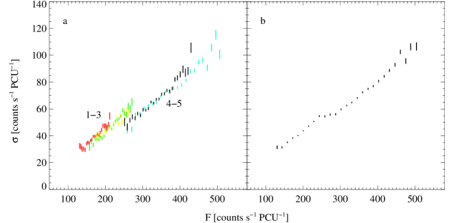
Figure 8: The observation of 2002 Feb 25 consists of five short segments 1–5. a) Segments 1–3 are at lower flux, while 4 and 5 are at higher flux, so that the rms-flux relations for each part are shifted with respect to each other. b) The superposition of all parts results in a “wavy” rms-flux relation. Error bars are at the 1$\sigma$ level.

To describe the flaring events when Cyg X-1 attempts the change from the common hard state into the soft state, without reaching the soft state, we coined the term “failed state transitions” (Pottschmidt et al. 2000; paper I). Depending on how far its state evolves, during these failed transitions Cyg X-1 can reach the intermediate state as defined by Belloni et al. (1996), or its behavior can remain hard state-like during these flares.

We examined four “failed state transitions” that were covered by RXTE observations in detail: 1998 July 15, 1999 December 05 (extracted as two separate lightcurve parts), 2000 November 03, and 2001 January 29 (probably a short soft state, see Cui et al., 2002). The values of $k$ and $C$ of the first failed state transition on 1998 July 15 are not different from the surrounding hard state observations. During the latter three failed state transitions, however, the values of $k$ and $C$ change to the soft state level. For one exemplary observation on 2000 November 03, this behavior is displayed in Fig. 7b. Comparing the failed state transition with the hard state observation immediately before (Fig. 7a), the rms-flux relation of 2000 November 03 changes to a lower slope and a small, negative intercept $C$ during the “failed state transition” itself. The PSD of this observation shows that this change in the rms-flux relation is accompanied by a decreasing Lorentzian component $L_{1}$ and an increasing Lorentzian component $L_{3}$ (Fig. 7d–e).

3.3 Spectral dependence of the rms-flux relation

We confirm a correlation between the photon spectral index, $\Gamma$, i.e., the hardness of the spectrum, and the mean rms, $\langle\sigma\rangle$, of the examined observations. In the hard state, the photon spectrum of each observation can roughly be described as the sum of a power law spectrum $E^{-\Gamma}$ with photon index $\Gamma$ and a multi-temperature disk black body (Mitsuda et al., 1984). The correlation of Fig. 9a takes into account only hard state and “failed state transition” observations and shows that $\langle\sigma\rangle$ increases as the spectrum grows softer. As rms variability and flux are linearly correlated in the hard state, this correlation between $\Gamma$ and $\langle\sigma\rangle$ is equivalent to a correlation between $\Gamma$ and flux. A similar result with RXTE ASM data of Cyg X-1 has been recently shown by Zdziarski et al. (2002), who found a very strong hardness-flux anticorrelation in the hard state.

Figure 9: a) Mean rms variability, $\langle\sigma\rangle$, b) slope, $k$, and c) flux intercept, $C$, as a function of photon spectral index, $\Gamma$, for failed state transitions and the hard state observations. Diamonds designate “failed state transitions”, crosses are for hard state observations. Error bars for $k$ and $C$ are given at the 90% confidence level for two interesting parameters.

We note that we are using the definition of paper I, using the term “failed state transitions” for those observations which exhibit a significantly increased time lag compared to its typical value, since the X-ray time lag seems to be a more sensitive indicator for state changes than the X-ray spectrum. As has been already been noted in Sect. 3.2 there are only four corresponding observations.

The filled diamond at $\Gamma\sim 2$ in Fig. 9 belongs to the “failed state transition” of 1998 July 15. The fact that this data point is situated within the value range of hard state observations in Figs. 4 and 9 confirms that this “failed state transition” has to be treated separately and classified as being close to the hard state, as already mentioned in Sect. 3.2. Allowing for the split in values of $k$ and $C$, respectively, between the hard state and failed state transition data, any correlation between the photon index and $k$, or $C$, cannot easily be detected.

Figure 10: Shape of a)-d) the rms-flux relation and e)-h) the corresponding PSD for the observation of 1999 May 21 for energy bands 2–5, respectively.

So far we concentrated on the rms-flux relation in the second lowest energy band, i.e., energy band 2 in the range $\sim$4–6 keV. This approach is justified as the linear rms-flux relation is found to be valid for all energy bands considered here (see, e.g., Fig. 10), such that the general behavior described for energy band 2 is also seen in the other bands. Even the rms-flux relation in energy band 3 which contains the iron K line does not show a different behavior, in agreement with the results of Maccarone & Coppi (2002a) that the iron line tracks the continuum at least in the soft and transition states. Nevertheless, there are subtle differences in the shape of the rms-flux correlation.

Comparing the values of $k$ and $C$ for the different energy bands, our energy resolved results for the rms-flux correlation show that $k$, which represents the fractional rms variability of the time variable component of the emission in the 1–32 Hz band, generally decreases with energy when the source is in the hard state (Fig. 11), in agreement with earlier results (e.g., Nowak et al., 1998). The same is true for $C$ (see Fig. 12). For the highest energy band 5, our analysis reveals that $k$ and $C$ only slightly correlate with energy band 2 (Figs. 11c and 12c). This result confirms earlier work claiming only a ‘loose coupling’ between the source variability at low and at high energies (Życki, 2003; Churazov et al., 2001; Maccarone et al., 2000; Gilfanov et al., 1999). In terms of Compton corona models, the fraction of photons from the accretion disk significantly decreases when proceeding from energy band 2 to energy band 5. Therefore we take our result to confirm earlier claims that the variability properties of Cyg X-1 are driven by coronal fluctuations and not by changes in the soft photon input to the putative Compton corona (Maccarone et al., 2000; Churazov et al., 2001, and references therein).

Figure 11: Slope of energy bands 3–5 plotted against the slope of energy band 2. The dotted line indicates $k_{i}=k_{2}$ where $i=\text{band\leavevmode\nobreak\ 3}$ through 5. Error bars are at the 90% confidence level for two interesting parameters.

Figure 12: Behavior of $C$ for energy bands 3 through 5, as a function of $C$ measured for energy band 2. The dotted line indicates $C_{i}=C_{2}$ where $i=\text{band\leavevmode\nobreak\ 3}$ through 5. Error bars are at the 90% confidence level for two interesting parameters.

To examine the overall spectral shapes of the two variability components characterized by $C$ and $k$, respectively, we plotted these values for the energy bands 2–5, normalising $C$ by $\langle F\rangle$ to account for the instrument response. Fig. 13 shows two examples with different photon spectral index, $\Gamma$. For most observations with $\Gamma$ lower than $\sim 2.0$, which means for the majority of hard state observations, the spectral shapes of $C$ and of $k$ are similar, but the spectral shape of $C$ tends to be somewhat flatter: both $C$ and $k$ show a soft energy spectrum, i.e., higher values at low energies and lower values at higher energies (Figs. 13a–b). When we proceed to higher $\Gamma$, observations begin to display a flat or even tilted spectrum, i.e. lower values at low energies and higher values at higher energies, more pronounced for $C$ than for $k$ (Figs. 13c–d). The change in the shape of the normalised $C$ (cf. Figs. 13a and c) is caused by the combination of an intrinsic change in the spectral shape of the unnormalised $C$ and a change in the spectral shape of $\langle F\rangle$. Suggestions that the two variability components $C$ and $k$, representing a constant and a variable rms component, will have basically different energy shapes cannot be confirmed, but to a certain degree in the low state the spectral shape of $C$ is flatter and harder than the spectral shape of $k$.

Figure 13: Spectral shapes of the two variability components characterized by $C$ and $k$, respectively. $C$ has been normalised by $\langle F\rangle$. a)-b) show a typical hard state observation (2001 April 7) with $\Gamma=1.89$, whereas c)-d) give an example of the tilted spectral shapes which can be found for higher $\Gamma$ (“failed state transition” observation of 2001 Jan 29 with $\Gamma=2.76$).

3.4 The rms-flux relation on short time scales

The fact that $\sigma$ tracks the flux implies that the “lightcurve” of the rms values is similar to the flux lightcurve. This fact can be used to probe how the rms responds to flux changes on short time scales (see also Uttley et al. 2003, in prep.). For example, if the rms does indeed track variations on all time scales, the PSD of the “rms lightcurve” should look similar to the PSD of the conventional “flux lightcurve”. In contrast, if the rms only tracks variations on time scales longer than, say, 10 s, the PSD of the rms lightcurve should be sharply cut off at 0.1 Hz. In order to test this issue we created 0.25 s lightcurve segments and calculated $F$ and $\sigma$ for each of these segments to make flux and rms lightcurves. From these lightcurves, we calculated the PSDs (shown for an arbitrarily chosen observation in Fig. 14). In this case, we do not correct the rms lightcurve for Poisson noise, since the stochastic nature of the noise process means that such a correction is only possible when averaging over comparably long time intervals. Note, however, that the effect of the Poisson noise and intrinsic noise contributions to the rms lightcurve is to add power to the rms PSD at high frequencies, not to cause spurious high-frequency cut-offs or breaks.

Figure 14: PSDs of a) $F$ lightcurve and b) $\sigma$ lightcurve for the hard state observation on 1999 July 05. The original flux lightcurve with time resolution of $\Delta t=2^{-8}$ s has been divided into 0.25 s segments, and the frequency range $\nu=4$–128 Hz was chosen for calculation of the rms variability of each segment. To compute PSDs from the flux and the rms lightcurves – consequently both with the time resolution of the segment length $\Delta t=0.25$ s – segments of 1024 time elements ($=1024\times 0.25\,\text{s}=256$ s) were used, thus resulting in a frequency range from $\nu_{\mathrm{min}}=0.004$ Hz to $\nu_{\mathrm{max}}=2$ Hz. We rebinned this range to 84 logarithmically spaced bins. c) Ratio of the $F$ lightcurve PSD to the $\sigma$ lightcurve PSD in order to quantify the similarity of the two PSDs.

Over the frequency range $\sim$0.01–0.2 Hz the rebinned PSDs show the same features as indicated by the flat ratio in Fig. 14c. Therefore it is likely that the rms-flux relation is fulfilled on time scales from 5 s to 100 s. Above 0.2 Hz, however, Poisson noise starts to dominate the rms PSD such that the shape of the rms and flux PSDs cannot be compared.

Similar tests dealing with the variability on different time scales have been discussed by Mineshige et al. (1994) and Maccarone & Coppi (2002b).

4 Discussion

4.1 The origin of the rms-flux relation

Uttley & McHardy (2001) have interpreted the rms-flux relation in terms of the disk fluctuation model of Lyubarskii (1997), where variations in the accretion rate occur at various radii and propagate inwards to modulate the X-ray emission. The fact that variations at larger radii should have longer characteristic time scales naturally explains the fact that the short term rms variations are modulated by longer time scale flux changes. As the slower variations in the accretion flow propagate inwards they are able to modulate the variations on shorter time scales. Kotov et al. (2001) have extended this model by introducing an extended X-ray emitting region with a temperature gradient, to explain the frequency dependent time lags between hard and soft bands observed in Cyg X-1 (Pottschmidt et al., 2000).

Churazov et al. (2001) have pointed out that in a standard thin disk, viscous damping will smooth accretion rate fluctuations on a viscous time scale, i.e., before they reach the inner disk, implying that for the Lyubarskii (1997) model to work, the fluctuations in accretion rate must happen in an optically thin or geometrically thick flow, such as an advection dominated accretion flow (ADAF) or another type of thick disk. We have shown that the linear rms-flux relation is seen in both high and low flux states, so that it very well might be associated with some component of the system that is common to both states. Since the X-ray variability during the soft state appears to be associated with the power law emission rather than thermal emission from the disk (which may be constant, Churazov et al., 2001), it seems likely that the rms-flux relation is associated directly with a corona which is present in both hard and soft states. We therefore speculate that the rms-flux relation in Cyg X-1 (and probably also other objects showing linear rms-flux relations) may present evidence for accretion rate variations in a fluctuating coronal accretion flow (see, e.g., Smith et al., 2002; van der Klis, 2001, and references therein). The suggestion that the corona itself accretes has been used to explain a number of observational features of both AGN and galactic BH systems (Witt et al., 1997), and since an optically thin coronal accretion flow is similar to an ADAF, such a model would not encounter the problems faced by a thin disk origin for the accretion variations (Churazov et al., 2001).

4.2 The long term rms-flux relation

In the previous sections we have shown that the linear rms-flux relation seems to apply on very long time scales, since the average 1–32 Hz rms of an observation scales linearly with the average flux of the observation. The hard and soft state data form two separate long term rms-flux relations, with different slopes $k_{\text{long}}$ (somewhat lower in the soft state, $k_{\text{long}}=0.19$ versus $k_{\text{long}}=0.22$ in the hard state). Intriguingly, the flux-offsets $C_{\text{long}}$ in the long term rms-flux relations of both hard and soft states are very close to zero, and certainly of much smaller amplitude than the typical offsets observed in the short term rms-flux relations of either state. The scatter in the hard state long term rms-flux relation is particularly small.

Combined with the almost-zero offset of the long term relation, this tight correlation implies that the fractional rms of the 1–32 Hz variability in the hard state is remarkably constant (similar to $k_{\text{long}}$, i.e., $\sim$22%). This result is rather surprising because the hard state PSD is clearly not stationary, i.e., the Lorentzians which successfully describe the PSD change significantly in both peak frequency and fractional rms (paper I). The most obvious example of such a change in the PSD can be seen in 1998 May (see paper I, Fig. 3) when the peak frequencies of the Lorentzians simultaneously increase, and the fractional rms of the $L_{3}$ Lorentzian (which lies between 3–10 Hz) and the fractional rms of the total PSD both decrease significantly. However, despite such a marked change in the PSD, the data before and after 1998 May lie along the same long term hard state rms-flux relation. The fact that the fractional rms in the 1–32 Hz band seems undisturbed by significant changes in the PSD suggests some sort of conservation of fractional rms at high frequencies, even though the low-frequency (and hence the total) fractional rms changes significantly. Although the specific 1–32 Hz band chosen to measure the rms-flux relation is somewhat arbitrary, we point out that the bulk of the power in this band is associated with the $L_{2}$ and $L_{3}$ Lorentzians, and the band fully encompasses the range of frequencies between 3–10 Hz in which a strong and well-defined anti-correlation between Lorentzian peak frequency and fractional rms is clearly seen (see paper I, Fig. 6). We suggest, therefore, that some process which conserves fractional rms above a few Hz may be at work, with fractional rms in the $L_{3}$ Lorentzian decreasing as the $L_{2}$ Lorentzian moves further into the 1–32 Hz band, resulting in a constant fractional rms in that band. We now examine how such a phenomenological model relates to the observed fundamental plane of short term rms-flux relation parameters $k$, $C$, and flux.

4.3 The hard state $k$-$C$-$\langle F\rangle$ fundamental plane

We have shown that the “fan shape” of the correlation between the rms-flux relation slope and its flux-offset in the hard state can be directly related to the long term rms-flux relation. The fact that $k$ and $C$ vary but the average 1–32 Hz rms must track the average flux explains the degeneracy in the correlation, which is the result of the various fluxes observed for a given pair of $k$ and $C$ values. Thus $k$, $C$, and $\langle F\rangle$ track out a fundamental plane which describes the forms the rms-flux relation can take in the hard state.

As noted by Uttley & McHardy (2001), $C$ can be interpreted either simply as a constant-flux component to the lightcurve, or as a constant rms component. We concentrate on these two interpretations since they are the simplest possibilities, but it should be emphasized that there are numerous other forms the variability could take, e.g., a component of constant fractional rms.

We have shown that, in the soft state at least, $C$ can be negative, which is only possible if the offset in this state represents a constant rms component. We argue that the existence of the $k$-$C$-$\langle F\rangle$ fundamental plane also suggests that $C$ represents a constant rms component in the hard state. For example, consider an increase in the slope $k$ between two observations, while keeping the average flux of the observations constant. The increase in $k$ corresponds to an increase in the fractional rms of the linear rms-flux component of the lightcurve. In order to maintain the constant total fractional rms as given by the observed long term rms-flux relation, $C$ must also increase. Therefore we suggest that both a constant rms component and a linear rms-flux component exist in the lightcurve and that the relative contribution of each varies in such a way that the sum of both components, the total fractional rms, is constant.

As a constraint to possible models it should be mentioned, as already noted in Sect. 3.3, that the spectral shapes of $k$ and $C$ are generally similar, with $C$ tending to a flatter/harder spectrum, and there is no obvious correlation between spectral index $\Gamma$ and $C$, $C_{\text{long}}$, and $k$, respectively.

4.4 Summary

To summarize, in this paper we analyzed Cyg X-1 lightcurves from 1996 to 2003 in an attempt to describe the long term evolution of X-ray rms variability. Our main results are

1. The linear rms-flux relation is valid throughout all states and energy ranges observed.

2. The slope of the linear rms-flux relation is steeper in the hard state than in the soft and intermediate states.

3. The rms-flux relation is valid not only on short time scales (seconds) but also on longer time scales (weeks–months).

4. In the hard state, the slope of the flux-rms-relationship is correlated with its flux intercept, but the correlation is increasingly degenerate at higher values of $k$ and $C$, forming a fan-like distribution in the $k$-$C$ plane. The hidden parameter governing the degeneracy is the long term average flux, $\langle F\rangle$, and the $k$-$C$-$\langle F\rangle$ relation maps out a “fundamental plane” in the low state.

5. The intercept of the linear rms-flux relation is relatively constant and positive in the hard state, but is diverse in the soft state: in the 1996 soft state $C$ is positive and slightly higher than during the hard state, in the atypical 2001/2002 “soft state” $C$ is decreasing relative to the hard state level, with several observations showing a negative $C$. During “failed state transitions”, $C$ is smaller than in the hard state, similar to the soft state behavior.

6. The $F$-$\sigma$-$\Gamma$ correlation can be confirmed for the hard state.

7. The clear dichotomy of $k$ in a hard and a soft state level in energy band 2 is weaker at higher energies.

Appendix A Buffer overflows in RXTE binned data modes

During phases of high soft X-ray flux, the rms-flux relation for energy band 1 ($\sim$2–4.6 keV) shows a clear deviation from its typical linear behavior. These phases are characterized by a smaller rms than what would be expected when extrapolating the rms-flux relation measured for smaller fluxes (Fig. 15). We initially associated this breakdown of the relationship with changes in the Comptonizing corona during phases of high luminosity (Gleissner et al., 2003), however, this interpretation was wrong.

Figure 15: In energy band 1 the rms-flux relation for observation 2000 Nov 03, just as several other high flux observations during intermediate and soft states, displays an “arch-like” form. The given error bars are at the 1$\sigma$ level.

Instead, the “arches” are caused by buffer overflows in the PCA hardware (see also Gierliński & Zdziarski, 2003; van Straaten et al., 2003). For the binned data mode B_2ms_8B_0_35_Q, with which most of our low energy data are taken, 4 bit wide counters are used to form the binned spectrum during each 2 msec binning interval. During phases of very high flux, which are especially likely during short outbursts possible during the failed state transitions, these buffers will overflow. Due to the softness of the X-ray spectrum during the failed state transitions, the likelihood for such overflows is highest in the lowest energy band. The buffer overflows become apparent when comparing the lightcurve of the binned data mode with the lightcurve as determined, e.g., from the GoodXenon data, which does not suffer from these problems. Except for phases of high flux, these lightcurves agree. During phases of high flux, however, multiples of 16 events are missing in the lightcurve from the binned data. Since the buffer overflows only occur for a few bins of the high resolution lightcurve, the flux determination is barely affected, however, the rms is reduced and “arches” such as that shown in Fig. 15 are observed. For the computation of the rms-flux relationship, we therefore resorted to using energy band 2, where the overall photon flux is lower and buffer overflows do not occur.

Note that GoodXenon data are not available for all observations considered here, furthermore, the energy resolution of the GoodXenon data is not good enough to allow the study of other timing parameters. We note that the rms-flux relationship is especially sensitive to buffer overflows as the data are sorted according to flux. For the determination, e.g., of power spectra, longer lightcurves are chosen, and the buffer overflows are only apparent in a slight change of the rms level of the power spectrum. Therefore, buffer overflows at the level seen in the data here only very slightly affect the normalization of the PSDs such as those used in paper I and do not have any influence on our earlier results.

References

- Belloni & Hasinger (1990) Belloni, T. & Hasinger, G. 1990, A&A, 230, 103
- Belloni et al. (1996) Belloni, T., Méndez, M., van der Klis, M., et al. 1996, ApJ, 472, L107
- Brocksopp et al. (1999) Brocksopp, C., Fender, R. P., Larionov, V., et al. 1999, MNRAS, 309, 1063
- Churazov et al. (2001) Churazov, E., Gilfanov, M., & Revnivtsev, M. 2001, MNRAS, 321, 759
- Cui et al. (2002) Cui, W., Feng, Y., & Ertmer, M. 2002, ApJ, 564, L77
- di Matteo & Psaltis (1999) di Matteo, T. & Psaltis, D. 1999, ApJ, 526, L101
- Dove et al. (1998) Dove, J. B., Wilms, J., Nowak, M. A., Vaughan, B., & Begelman, M. C. 1998, MNRAS, 289, 729
- Fender (2002) Fender, R. 2002, in LNP Vol. 589: Relativistic Flows in Astrophysics, 101
- Gierliński & Zdziarski (2003) Gierliński, M. & Zdziarski, A. A. 2003, MNRAS, 343, L84
- Gierlinski et al. (1998) Gierlinski, M., Zdziarski, A. A., Coppi, P. S., et al. 1998, in The Active X-ray Sky: Results from BeppoSAX and RXTE, ed. L. Scarsi, H. Bradt, P. Giommi, & F. Fiore, Nuclear Physics B Proc. Supp. (Elsevier Science), 312
- Gilfanov et al. (1999) Gilfanov, M., Churazov, E., & Revnivtsev, M. 1999, A&A, 352, 182
- Gleissner et al. (2003) Gleissner, T., Wilms, J., Pottschmidt, K., et al. 2003, in New Views on Microquasars, ed. P. Durouchoux, Y. Fuchs, & J. Rodriguez (Kolkata: Centre for Space Physics), 46
- Jahoda et al. (1996) Jahoda, K., Swank, J. H., Giles, A. B., et al. 1996, in EUV, X-Ray, and Gamma-Ray Instrumentation for Astronomy VII, ed. O. H. Siegmund, & M. A. Gummin, Proc. SPIE Vol. 2808 (Bellingham, WA: SPIE), 59
- Keeping (1962) Keeping, E. S. 1962, Introduction to statistical inference (Princeton: Van Nostrand)
- Kotov et al. (2001) Kotov, O., Churazov, E., & Gilfanov, M. 2001, MNRAS, 327, 799
- Levine et al. (1996) Levine, A. M., Bradt, H., Cui, W., et al. 1996, ApJ, 469, L33
- Lochner et al. (1991) Lochner, J. C., Swank, J. H., & Szymkowiak, A. E. 1991, ApJ, 376, 295
- Lyubarskii (1997) Lyubarskii, Y. E. 1997, MNRAS, 292, 679
- Maccarone & Coppi (2002a) Maccarone, T. J. & Coppi, P. S. 2002a, MNRAS, 335, 465
- Maccarone & Coppi (2002b) Maccarone, T. J. & Coppi, P. S. 2002b, MNRAS, 336, 817
- Maccarone et al. (2000) Maccarone, T. J., Coppi, P. S., & Poutanen, J. 2000, ApJ, 537, L107
- Mineshige et al. (1994) Mineshige, S., Takeuchi, M., & Nishimori, H. 1994, ApJ, 435, L125
- Mitsuda et al. (1984) Mitsuda, K., Inoue, H., Koyama, K., et al. 1984, PASJ, 36, 741
- Miyamoto et al. (1992) Miyamoto, S., Kitamoto, S., Iga, S., Negoro, H., & Terada, K. 1992, ApJ, 391, L21
- Novikov & Thorne (1973) Novikov, I. D. & Thorne, K. S. 1973, in Black Holes — Les Astres Occlus, ed. C. DeWitt & B. DeWitt (New York, London: Gordon and Breach), 345
- Nowak (2000) Nowak, M. A. 2000, MNRAS, 318, 361
- Nowak (2003) Nowak, M. A. 2003, in New Views on Microquasars, ed. P. Durouchoux, Y. Fuchs, & J. Rodriguez (Kolkata: Centre for Space Physics), 11
- Nowak et al. (1998) Nowak, M. A., Dove, J. B., Vaughan, B. A., Wilms, J., & Begelman, M. C. 1998, in The Active X-ray Sky: Results from BeppoSAX and RXTE, ed. L. Scarsi, H. Bradt, P. Giommi, & F. Fiore, Nuclear Physics B Proc. Supp. (Elsevier Science), 302
- Nowak et al. (1999) Nowak, M. A., Vaughan, B. A., Wilms, J., Dove, J. B., & Begelman, M. C. 1999, ApJ, 510, 874
- Nowak et al. (2002) Nowak, M. A., Wilms, J., & Dove, J. B. 2002, MNRAS, 332, 856
- Pottschmidt et al. (2000) Pottschmidt, K., Wilms, J., Nowak, M. A., et al. 2000, A&A, 357, L17
- Pottschmidt et al. (2003) Pottschmidt, K., Wilms, J., Nowak, M. A., et al. 2003, A&A, 407, 1039 (Paper I)
- Psaltis & Norman (2001) Psaltis, D. & Norman, C. 2001, ApJ, submitted (astro-ph/0001391)
- Scarsi et al. (1998) Scarsi, L., Bradt, H., Giommi, P., & Fiore, F., eds. 1998, The Active X-ray Sky: Results from BeppoSAX and RXTE, Nuclear Physics B Proc. Supp. (Elsevier Science)
- Shakura & Sunyaev (1973) Shakura, N. I. & Sunyaev, R. A. 1973, A&A, 24, 337
- Shapiro et al. (1976) Shapiro, S. L., Lightman, A. P., & Eardley, D. M. 1976, ApJ, 204, 187
- Smith et al. (2002) Smith, D. M., Heindl, W. A., & Swank, J. H. 2002, ApJ, 569, 362
- Sunyaev & Trümper (1979) Sunyaev, R. A. & Trümper, J. 1979, Nature, 279, 506
- Thorne & Price (1975) Thorne, K. S. & Price, R. H. 1975, ApJ, 195, L101
- Uttley & McHardy (2001) Uttley, P. & McHardy, I. M. 2001, MNRAS, 323, L26
- van der Klis (1989) van der Klis, M. 1989, in Timing Neutron Stars, ed. H. Ögelman & E. P. J. van den Heuvel, NATO ASI No. C262 (Dordrecht: Kluwer Academic Publishers), 27
- van der Klis (1995) van der Klis, M. 1995, in X-ray Binaries, ed. W. H. G. Lewin, J. van Paradijs, & E. P. J. van den Heuvel (Cambridge: Cambridge University Press), 252
- van der Klis (2001) van der Klis, M. 2001, ApJ, 561, 943
- van Straaten et al. (2003) van Straaten, S., van der Klis, M., & Méndez, M. 2003, ApJ, 596, 1155
- Witt et al. (1997) Witt, H. J., Czerny, B., & Życki, P. T. 1997, MNRAS, 286, 848
- Zdziarski et al. (2002) Zdziarski, A. A., Poutanen, J., Paciesas, W. S., & Wen, L. 2002, ApJ, 578, 357
- Życki (2003) Życki, P. T. 2003, MNRAS, 340, 639