A new paradigm for the universe
primarymsc200085A40 \subjectsecondarymsc200083C57 \subjectsecondarymsc200085A15 \subjectsecondarymsc200085A05 \subjectsecondarymsc200083F05 \makeopinert \makeopIF \makeopNM \makeopSO \makeopdeS \makeopRic \makeopdiv \makeopExp \makeopIsom \makeopCont \makeopconst
A new paradigm for the universe
Colin Rourke
This is arXiv version 5 of “A new paradigm for the universe”
arxiv.org/abs/astro-ph/0311033v5
also available from the author’s web page
The most up-to-date version is available from Google Play and from Amazon in Kindle format and as a paperback with publication data:
ISBN: 9781973129868\nlImprint: Independently published\nl
Foreword
The universe is a wonderful, amazing place. We know a lot about it through a series of fantastic observations using ground and space based telescopes and other equipment, including recently, equipment to detect gravitational waves. There is a consensus model (the “standard model”) for the way it works which starts with the “Big Bang” and expands … BUT there are several unsatisfactory features to this model and the purpose of this book is to present a complete new model which fits all the observations and does not share these unsatisfactory features.
The main unifying idea of this book is that the principal objects in the universe form a spectrum unified by the presence of a massive or hypermassive black hole. These objects are variously called quasars, active galaxies and spiral galaxies. The key to understanding their dynamics is angular momentum and the key tool, and main innovative idea of this work, is a proper formulation of “Mach’s principle” within Einstein’s theory of General Relativity (EGR) using Sciama’s ideas.
In essence, what is provided here is a totally new paradigm for the universe. In this paradigm, there is no big bang, and the universe is many orders of magnitude older than current estimates for its age. Indeed there is no natural limit for its age. The new model for the underlying space-time of the universe is based on a relativistic analogue of the sphere, known as de Sitter space. This is a highly symmetrical space which makes the model fully Copernican in both space and time, in other words the universe looks much the same in the large at any place or time. By contrast the current standard model of mainstream cosmology is Copernican only in space and not in time. This means that the view of the universe expounded here is similar to the steady state theory proposed and defended by Fred Hoyle (and others) in the last century, but it is not the same as their theory, which proposed an unnatural continuous creation hypothesis; like the big bang, this hypothesis breaks commonly accepted conservation laws.
It is worth mentioning that, by contrast with many attempts to find a model for the universe with no big bang, this book does not propose any new physics. It fits squarely within EGR. But it is necessary to make a new hypothesis for the inertial dragging effect of rotation in order to formulate the version of Mach’s principle needed (Sciama’s principle) within the framework of EGR. This formulation solves one of the main philosophical objections to Mach’s principle namely the causal problems that a naive formulation runs into.
AMS classification \@primclass; \@secclass\np
Preface
I started with the intention of writing a book intelligible to a general reader with a scientific interest. Some of the material that I wrote in this endeavour is included as \fullrefapp:beginners “Introduction to relativity”. Readers who have little previous knowledge, or wish to have their basic knowledge refreshed, should read this appendix before the main text.
However I quickly realised that the main material of the book is far too technical to treat at an elementary level in a book of modest proportions and I have not tried to avoid technicalities in the main body of the text. But I have tried to make the introductory parts of the book and of each chapter accessible to a general reader and I hope that a reader who has only a little technical knowledge will be able to find sufficient material to read to understand the main ideas presented here.
Several parts of this book are based on joint work with Robert MacKay and I thank him for allowing me to use this material and also for a thoughtful critical read. I would also like to thank Rosemberg Toala Enriques for the use of the material in the draft three author paper [BHQR] on quasars. Special thanks are due to Robert MacKay, Ian Stewart and Rob Kirby for unfailing support through the discouraging process of attempting to publish this work in serious scientific journals. It seems that self-publishing is the only vehicle open to an author who challenges the received orthodoxy.
Colin Rourke\nlOctober 2017\nl\nlMathematics Institute, University of Warwick, Coventry CV4 7AL, UK\nlcpr@msp.warwick.ac.uk http://msp.warwick.ac.uk/~cpr
About the author
![[Uncaptioned image]](/html/astro-ph/0311033/assets/figs/cpr.jpg)
Colin Rourke is a professor emeritus of mathematics at the University of Warwick, and has also taught at the Princeton Institute for Advanced Study, Queen Mary College London, the University of Wisconsin at Madison, and the Open University, where he masterminded rewriting the pure mathematics course; he has recently retired from lecturing after completing a half-century (of 50 years of lecturing). He has written papers in high-dimensional PL topology, low-dimensional topology, combinatorial group theory and differential topology.
In 1996, dissatisfied with the rapidly rising fees charged by the major publishers of mathematical research journals, Colin decided to start his own journal, and was ably assisted by Rob Kirby, John Jones and Brian Sanderson. That journal became Geometry & Topology. Under Colin’s leadership, GT has become a leading journal in its field while remaining one of the least expensive per page. GT was joined in 1998 by a proceedings and monographs series, Geometry & Topology Monographs, and in 2000 by a sister journal, Algebraic & Geometric Topology. Colin wrote the software and fully managed these publications until around 2005 when he cofounded Mathematical Sciences Publishers (with Rob Kirby) to take over the running. MSP has now grown to become a formidable force in academic publishing. With his wife Daphne, he runs a smallholding in Northamptonshire, where they farm Hebridean sheep and Angus cattle.
In 2000 he started taking an interest in cosmology and published his first substantial foray on the ArXiv preprint server in 2003. For the past ten years he has collaborated with Robert MacKay also of Warwick University with papers on redshift, gamma ray bursts and natural observer fields. He now feels that he has mastered the basis of a completely new paradigm for the universe without either dark matter or a big bang. This new paradigm is presented in this book.
Photo: Pip Sheldon
Chapter 1 Introduction
Cosmology – the study of the universe in the large – is a topic which arouses a great deal of public interest, with serious articles both in the scientific press and in major newspapers, with many of the theories and concepts (eg the “big bang” and “black holes”) discussed, often in depth. The observations that support these discussions use sophisticated and expensive machinery both on the earth (eg the LIGO equipment used to detect gravitational waves) and in orbit around the earth (eg the Hubble telescope). There is a consensus for the theoretical framework supporting and interpreting these observations, which is known as the “standard model”. It starts with the big bang and expands from there to fill the entire visible universe. The image presented is of a complete and full theory that (with a few minor unsolved problems) explains all the observations that we have.
This image is (like many images) completely false. There are huge problems with the standard model, some of which will be discussed shortly. It is the aim of this book to present an alternative model to the standard one, which avoids the most glaring of these problems. The model is complete in outline with several topics covered in full detail, including the dynamics of galaxies and the nature of quasars.
1.1 Two philosophical problems
There are two major philosophical problems with the standard model. Firstly it is based directly on Einstein’s theory of “General Relativity” (hereinafter referred to as EGR) which does not satisfy “Mach’s principle” in general. This principle centres around the philosophically compelling idea that the concept of acceleration or rotation must be connected to the main distant mass of matter in the universe. Rotation is the simplest to think about. An observer can tell that he is rotating without leaving his closed windowless spaceship, because there are forces that he experiences (for example Coriolis force) that he does not experience if he is not rotating. But what possible difference is there between him rotating, and him being still with the universe rotating around him? The conclusion is that the forces he experiences are due to some mysterious effect of the rotation of the universe around him. These considerations have passed into general circulation as “Mach’s principle” which is usually summarised as stating that the local concept of inertial frame (a frame in which there is no acceleration or rotation) is correlated with the distribution and motion of all the matter in the universe. Any theory which aims to accurately describe the universe must have such a property in some form. EGR does not.
The second problem is the (again philosophically compelling) principle known as the Copernican (or cosmological) principle. This is the principle that no particular location should be special. There is no centre to the universe: no “fingers of God”. This should also be true of time as well as space, there should be no special times: we should not live in a special time any more than we live in a special place. This space-time non-speciality principle will be called the “Perfect Copernican Principle” or PCP (which can also be read as the “Perfect Cosmological Principle”).
Obviously the current consensus model does not satisfy this principle because it starts with a very special event, the big bang, taking place at a very special time.
1.2 Dark matter
There are two other major problems. The first (the so-called “dark matter” problem) is recognised as a major problem, whilst the second (the “Arp problem”) is not recognised but ought to be. The dark matter problem arises from the observed rotation curves for galaxies. Typically the curve (of tangential velocity against distance from the centre ) comprises two approximately straight lines with a short transition region. The first line passes through the origin, in other words rotation near the centre has constant angular velocity (plate-like rotation); the second is horizontal, in other words the tangential velocity is asymptotically constant, see \fullreffig:modbeg (right). Furthermore, observations show that the horizontal straight line section of the rotation curve extends far outside the limits of the main visible parts of galaxies and the actual velocity is constant within less than an order of magnitude over all galaxies observed (typically between 100 and 300km/s) see \fullreffig:rotsSR.
Galactic rotation curves are so characteristic (and simple to describe) that there must be some strong structural reason for them. They are very far indeed from the curve obtained with a standard Keplerian model of rotation under any reasonable mass distribution. In a Keplerian model if is asymptotically constant then the mass inside radius is asymptotically equal to a constant times and tends to infinity with .
Nevertheless, in spite of the huge mass needed, a Keplerian model is exactly what is assumed in the consensus model. To square the circle, current theory hypothesises the existence of a huge amount of matter. Since this matter is not observed, it is called called “dark”. It needs to be distributed in precisely the right way to make Keplerian rotation fit the rotation curve. This is extremely implausible for several reasons which will be discussed in \fullrefsec:rot_curve. There is also a companion problem for the dynamics of spiral galaxies. The standard model has no satisfactory model for galactic dynamics which explains the persistent spiral structure widely observed. The new model presented here solves the dark matter problem and gives a full model for galactic dynamics. It does this by building a limited version of Mach’s principle into EGR (and this also deals with the first philosophical problem). In essence all that is needed is to use a suitable relativistic model instead of a Keplerian one.
In passing, it is worth mentioning that there is another “problem” often mentioned, namely “dark energy”. The author’s view is that there is no problem here. Dark energy is just a name for the term in the field equations that provides global curvature. It is not a problem any more than the curvature of the earth’s surface is a problem: it is just part of the description of the universe!
1.3 The Arp problem
Halton Arp was a talented observer who provided key observations supporting Hubble’s theory of the expanding universe. He also observed many examples of quasars with intrinsic (gravitational) redshift against the current mainstream dictat that all redshift must be cosmological. A particularly striking example is reproduced in \fullreffig:NGC7603. It is commonsense that the alignments seen in this configuration of galaxies and quasars are not due to chance and there are many similar such in Arp and other’s observations [Arp, Getal]. Objects 2 and 3 (quasars) have cosmological redshift around (for the filament) and the remainder must be instrinsic (presumably gravitational). As often happens when a consensus view is challenged by direct evidence, the evidence is ignored and the challenger discredited. Arp was sidelined by the mainstream cosmological community and denied observation time on the big telescopes. One of the main aims of this book is to rehabilitate Arp’s reputation (unfortunately posthumous), and if it succeeds in this aim it will have been worth writing. As will be seen later, it is in fact quite easy to correct the standard model for quasars to allow for instrinsic redshift, indeed, once again, the correction is to use a simple piece of relativistic geometry.
1.4 A little history
It is worth giving a quick history of cosmology to explain how the current theory has become stuck in a groove of self-justifying explanations which deny the reality of evidence that contradicts the consensus view. One problem has already been hinted at. Despite being nominally based on General Relativity, the theory tends to opt for non-relativistic models (such as the Keplerian model for galactic rotation) and avoid the flexibility offered by fully relativistic models. Another example is the universal time assumed in the standard model in contrast to the relativistic nature of time (depending on the observer) in general relativity. Without a universal time, the observations of expansion do not imply that the universe must have started with a big bang.
Cosmology arose directly from Einstein’s theory of general relativity. This theory is so beautiful and well-formed that it rapidly became accepted as the basic geometry of the universe. Einstein himself started model building very early in the development of the theory. He became obsessed with the problem of finding a static solution to his equations and introduced his “cosmological constant” in order to do this. Incidentally this constant is the source of “dark energy” mentioned earlier. He built models based on the simplest manifolds for space (flat space or the 3–sphere) with a universal time parameter. These models, which should by now have been discarded as overly simple, have stuck and the current standard model also uses very simple manifolds with a universal time parameter. It is the over simplicity of the models used which leads to the fallacy that observed expansion implies global expansion which in turn implies the big bang.
This happened despite the model proposed early on by Willem de Sitter who collaborated with Einstein. This is the analogue in space-time of a sphere in ordinary space and has a similarly complete set of symmetries: there is a symmetry that carries any point to any other and indeed one that carries any time-like geodesic to any other and hence this model has the PCP. It fits Einstein’s equations (with cosmological constant) and there is no big bang. Unfortunately for cosmology, de Sitter space was abandoned as a model for the universe very early in its development. De Sitter himself used a very unnatural metric which obscured the symmetry and an influential mathematician, Hermann Weyl, proposed a widely accepted “coherency postulate” [We] which supposes that no astronomical object can suddenly appear into view or has so appeared at a finite time in the past. All must have been always visible. This cuts de Sitter space down to just the expanding frame based on the home geodesic (the one on which our galaxy is travelling) and loses the PCP. It makes the point at time on the home geodesic a special point: the universe seems to have this point as an origin, see \fullreffig:Mosch (left). In this figure the blue lines are geodesics along which objects permitted by Weyl’s hypothesis are travelling, with the central one being the home geodesic. The black lines are transverse (flat) space slices. Thus the hypothesis leads the way to the current “standard models” which start with a Big Bang at a finite time in the past.
Another early model with the PCP was the Bondi–Gold–Hoyle steady state theory (SST): this hypothesises that matter is created by empty space at exactly the correct rate to compensate for the observed Hubble expansion – a hypothesis also briefly toyed with by Einstein (see [ESS]) as a possible alternative to (or explanation of) the cosmological constant, as a means of attaining a static solution to the field equations. Hoyle was an energetic proponent of this theory against the Big Bang theory (a sarcastic name that he invented) and his writings on the subject are well worth revisiting. Eventually he gave way because of the evidence of historic change in the composition of the universe from quasar observations – evidence that was in fact badly misinterpreted, see \fullrefsec:killam and \fullrefsec:quasars. Hoyle’s SST could still be correct and in deference to his enthusiasm, a model with the PCP will be called a “Hoyle Universe”. The model outlined in this book, based on de Sitter space, is indeed a Hoyle Universe, but it does not have the unnatural continuous creation hypothesis of the SST, which, like the Big Bang breaks commonly accepted conservation laws.
For more (or perhaps better) history the reader is directed to [Longair, Chapter 1].
1.5 The quasar–galaxy spectrum
A major theme of this work is that there is a spectrum of related phenomena. This is the quasar–galaxy spectrum. The unifying element is the presence of a massive (or hypermassive) black hole. The position of a quasar or galaxy on the spectrum is determined entirely by the size of this associated black hole, which varies from solar masses (sm), or less, for a small quasar such as Sagittarius , through to sm for a so-called active galaxy and up to sm, for a full size mature spiral galaxy. An aside here: the phrase “so-called” for active galaxies is used because one of the main theses of this work is that all galaxies are highly active and that, for spiral galaxies, this activity manifests itself in the very spiral structure that characterises them.
These phenomena are systematically misunderstood in the consensus theory. At the smaller end, the quasar end, there is an observed redshift which can be very large (up to or more—much more as will be seen later) and, for reasons which will be explained shortly, the current mainstream view is that this redshift is entirely cosmological (due to the expansion of the universe). This implies that these objects are very distant, extremely massive, created just after the big bang and have a truly phenomenal power output, which is very hard to explain. One of the major tasks of this work is to explain how this view has arisen and how it can be changed to the view that, by contrast, quasars are typically small, nearby objects with a modest power output easily modelled by a simple spherical accretion mechanism.
The key to this misunderstanding and to the correct model for quasar energy production is angular momentum. Very early in the study of quasars it was decided that the behaviour of angular momentum gives a compelling reasons for believing that quasar redshift is cosmological. Quasars are typically believed to be based around a very dense object, probably a black hole, and their energy production is believed to be due to accretion from the surrounding medium. Particles fall into the gravitational well of the central mass and the gravitational energy is released by interaction between different infalling particles. Now given a small but very heavy object, a particle approaching with a small tangential velocity will have its tangential velocity magnified by conservation of angular momentum and there will be a radius of closest approach. It is very unlikely to actually fall into the central gravitational well.
The same thing happens for the full flow of infalling matter from the surrounding medium which will typically have a nonzero angular momentum around the black hole. This gives an obstruction to accretion which was found not long after quasars were discovered, for example Michel [michel, Section 4, p 158] (1976) states:
…One must, however, somehow transfer away most of the angular momentum that the infalling gas had relative to the centre of mass. It seems physically plausible that the effect of such angular momentum would be to choke down the inflow rates. For example, even when magnetic torques are included …one finds that the ‘infall’ solutions terminate at finite distances from the origin in analogy with the minimum approach distance of a single particle trajectory having non-zero initial angular momentum. …
These considerations have led to the subject being dominated by the theory of “accretion discs”. The idea is that, since infalling matter cannot flow smoothly into the central black hole, it must typically settle into a rotating structure of some kind, which is called (whatever its actual shape) an accretion disc. Then interaction between infalling matter and this structure allows energy to be produced.
A consequence of this is that redshift, which is frequently observed in quasar radiation, is generally believed to be cosmological and not gravitational (or intrinsic). Indeed if the observed radiation comes from an accretion disc and the redshift is caused by the gravitational field of the nearby black hole, then because the disc varies in its distance from the black hole over its extent, the spectral lines observed would be wide (a phenomenon known as “redshift gradient”) and not the narrow lines that are observed.
This in turn implies that the universe has varied in its constitution over the observable past. As remarked above, a quasar with a large cosmological redshift must be a massive object with a huge energy output. But there are no observations of huge sources of energy close to us like these (supposed) near the big bang. This provides strong supporting evidence for the big bang theory, which entails a continuous change in the constitution of the universe. A steady state model cannot contain a big bang.
It was considerations like these that caused Fred Hoyle to abandon his continuous creation model which is fully Copernican in both space and time, ie with no observable global change over time.
1.6 Killing the angular momentum obstruction
One of the main theses of this book is that the angular momentum obstruction to accretion can be killed by the black hole itself and this implies that quasars can be relatively small, nearby objects and the universe could be Copernican in time as well as space. Thus Hoyle’s model could still be correct (though it is not the model proposed here).
The key to killing this angular momentum obstruction is to work in a relativistic framework and not the Newtonian framework implicitly assumed in the above discussion. A relativistic effect—the dragging of inertial frames, abbreviated to “inertial drag”—allows the black hole to compensate for the angular momentum of the infalling gasplasma stream and for an energy production model to be established with radiation coming from a thin spherical region (the Eddington sphere) which can be very close to the event horizon of the black hole and subject to an arbitrarily high gravitational redshift, with the cosmological redshift small in comparison. Because the production sphere is thin, there is little redshift gradient.
As mentioned above there is some very strong evidence in the observations of Arp and others [Arp, Getal] that quasars do in fact possess intrinsic, ie gravitational, redshift. This and the angular momentum considerations just mentioned led Arp to propose some fantasy physics explanations for this redshift. The explanation proposed in this work uses only well-accepted (and definitely not fantasy) physics and is fully consistent with Arp’s observations.\fnoteThe one new hypothesis that is made in this work, the inertial drag force, see below, does not play any role in this explanation.
1.7 Embedding Mach’s principle in EGR
Alongside inertial drag, the other main ingredient for the new paradigm presented in this book is “Mach’s principle” outlined above. It is necessary to explain how to embed the version of Mach’s principle that is needed for this work into EGR (Einstein’s General Relativity). There are obvious causal problems in a naive statement: how exactly does distant matter communicate with local matter to determine the local inertial frame? and does the influence happen instantaneously or travel at the speed of light? These problems will be avoided by restricting to a limited version of the principle due to Sciama [Sciama] which is quantitative rather than philosophical and which is referred to as Sciama’s principle. The discussion is further simplified by concentrating on rotation at the expense of general non-inertial motions. EGR deals well with acceleration, so this makes sense for the purposes of embedding the principle within EGR.
A new hypothesis is needed for the dragging effect of a rotating body on the inertial frames near it. The precise behaviour that is needed is not a consequence of Einstein’s equations and the hypothesis amounts to assuming that a rotating mass has a non-zero effect on the stress-energy tensor near it – in other words stops the space near it being a true vacuum. This gives a natural way to understand how inertial drag propagates: the disturbance to the local vacuum is akin to a gravity wave and propagates at the speed of light. Furthermore reading back from the rest of the universe, the local background inertial frame is created by the rest of the universe by a similar propagation effect from all the rest of the matter (a brief aside here: this makes sense only if the sum is finite – or quasi-finite – this will be explained in the next chapter).
It is worth briefly comparing the new inertial drag hypothesis made in this book with the dark matter hypothesis made in current mainstream cosmology. At first sight they may appear to be similar. Both correct the rotation curve for galaxies. But the dark matter hypothesis amounts to assuming the existence of inert matter, which has no effect other than gravitational attraction, and cannot otherwise be detected. The inertial drag hypothesis on the other hand amounts to assuming a new effect of a rotating body on the field outside it. It embodies a limited version of Mach’s principle which, as has been seen, is philosophically compelling, and must be embodied in any theory that seeks to accurately describe reality. Thus, unlike the dark matter hypothesis, the inertial drag hypothesis is a necessary part of a complete theory. Furthermore, the inertial drag hypothesis also underlies a good model for the dynamics of spiral galaxies, whereas the dark matter hypothesis leaves this problem unsolved. More detail on this point will be given later in the book (\fullrefsubsec:Add).
1.8 Outline of the rest of the book
Mach’s principle is discussed in \fullrefsec:Sciama, after which \fullrefsec:rot_curve derives the inertial drag effect, that allows quasars to cancel out the angular momentum obstruction to accretion, and fuels the dynamics of galaxies. In this chapter it is applied to model the rotation curve for galaxies without needing “dark matter”.
Next in \fullrefsec:quasars the subject of quasars is taken up in earnest. Here it is explained how inertial drag allows black holes to absorb the angular momentum in infalling gasplasma and to grow by accretion. The spherical accretion model that this allows is joint work with Rosemberg Toala Enriques and Robert MacKay [BHQR]. This work is still in draft form, but nevertheless the model fits observations extremely well, including those of Arp [Arp], and also explains the apparently paradoxical results of Hawkins [H]. This section contains a first description of the pivotal quasar–galaxy spectrum. Technical details from [BHQR] are deferred to \fullrefapp:3author.
After this the second main task of the book is tackled in \fullrefsec:spiral_struc, namely to provide a model for the spiral structure of full-size galaxies, such as the Milky Way, which lie at the other end of the quasar–galaxy spectrum. The nature of these objects is also much misunderstood by mainstream cosmology. Spiral galaxies all contain a central hypermassive black hole (of mass sm or more), which controls the dynamic by the same inertial drag effect that allows accretion in quasars, and which is surrounded by an accretion structure responsible for generating the visible spiral arms. Another aside here: there is a special misunderstanding with the Milky Way, where Sgr with a mass of only sm, far too light to have any dynamic effect on the galaxy, is believed to be the central black hole. This misunderstanding will be cleared up at a later stage.
Between quasars and spiral galaxies lie “active” galaxies for which accretion structures have been directly observed. This is the only part of the quasar–galaxy spectrum which is more-or-less correctly understood by mainstream cosmology. There will be a lot more to say about the whole quasar–galaxy spectrum later in this work.
As mentioned above, there is, inside a full size spiral galaxy, an accretion structure, called “the generator”, which is responsible for generating the spiral arms. This is described in \fullrefsec:spiral_struc where a full model for the resulting spiral structure is derived. The generator feeds the roots of the spiral arms with a pure light element mixture (H and He with a trace of Li). This is the same mixture of elements that is hypothesised to have been created in the big bang just before the time of the last scattering surface from the cooling of a hot plasma of quarks, and the process is similar. The residue of these streams, not condensed into stars, escapes the galaxy and feeds the intergalactic medium and this explains the observed proportion of these elements in the universe (which is one of the so-called “pillars of the big bang theory”).
sec:obs and \fullrefsec:cosm cover observations and consequences for cosmology. Included here are a comprehensive rebuttal of the big bang theory and explanations for redshift and the Cosmic Microwave Background (CMB), which are the other two pillars. There is also an explanation for Gamma Ray Bursts (GRB). Technical details for several of the topics are again deferred to appendices.
Chapter 2 Sciama’s principle
This chapter is concerned with a discussion of Mach’s principle and the restricted version that is needed for the dynamical applications (to quasars and spiral galaxies) in the rest of the book. The final form of the principle (the Weak Sciama Principle) hypothesises an inertial dragging effect from a rotating body which drops off asymptotically with where is a constant and is distance from the centre. A reader who is happy to accept this principle can omit this chapter without loss. The precise assumption is repeated near the beginning of the next chapter.
2.1 Inertial frames and Mach’s principle
In any dynamical theory there are certain privileged frames of reference in which the laws of Newtonian physics hold to first order. These frames are variously called “inertial frames” or “rest frames”. They are characterised by a lack of forces correlated with acceleration or rotation. In Newtonian physics there is a universal inertial frame referred to as “absolute space” and in Minkowski space the standard coordinates provide an inertial frame at the origin. Then Lorentz transformations carry this frame to an inertial frame at any other point, providing inertial frames for special relativity. General relativity is built on Minkowski space which in turn provides inertial frames for this theory, see \fullrefsec:genrel. Berkeley [Berkeley] and Mach [Mach] criticised Newton’s assumption of absolute space. Berkeley suggested that the local rest frame could be defined by distant “fixed” stars. Mach’s book [Mach, Ch II.VI (p 271 ff)] contains a devastating critique of Newton’s assumptions and is well worth reading. It was extremely influential and Einstein acknowledged a debt to his ideas. Mach’s basic point is that one should never assume anything that is not directly connected to observations of some kind and in particular the concept of the local inertial frame must be defined in terms of (theoretically) observable quantities. Some detail from Mach is given in \fullrefsh:Mach below.
The basic property of inertial frames is that they are only defined up to uniform linear motion. Given any inertial frame, a frame which is in uniform linear motion with respect to the given frame is also an inertial frame. Thus “the” inertial frame at a point in fact means an equivalence class of frames, two frames in the class being in mutual uniform linear motion with respect to each other. (For this reason, calling them “rest” frames is highly misleading and this terminology will not be used again.)
Mach’s ideas have passed into general circulation as “Mach’s principle” which is usually summarised as stating that the local concept of inertial frame is correlated with the distribution and motion of all the matter in the universe. However there are many other ways of interpreting the principle and there is a huge literature on the subject. At its weakest, the principle is interpreted as merely stating that all phenomena must have their origin in some material source (see eg [SWG]), and it has even been interpeted as an assumption about the nature of the big bang (Tod [Tod]).
For the purposes of this book, a statement is needed which is more precise than these but not so wide ranging. What is needed is a local version which applies to rotation of inertial frames and which is quantified precisely.
2.2 Sciama’s principle
The version that is used is close to the version in Sciama’s thesis [Sciama]. Sciama makes a bold attempt to base a full theory of dynamics on Mach’s principle. His idea is that the inertial frame at any point in the universe is determined by the inertial frames at every other point . The contribution from is nonzero only if there is a mass at and then the contribution is (a) proportional to this mass and (b) inversely proportional to the distance between and . In other words the contribution is
where means the inertial frame at . The idea is that this should be summed over “all the matter in the universe”.
To make sense of this sum it is necessary to make a number of assumptions. Firstly, in order to add up contributions, it is necessary to work in a linear framework and the simplest way to do this is to work with a perturbation of flat (Minkowski) space, which is exactly what Sciama does. The underlying Minkowski space provides “standard” reference frames at each point and the motion of any frame can be measured with respect to this standard, and also provides a space in which to measure the distance used in the summation.
Working within a perturbation of Minkowski space limits the theory to weak fields, but it suffices for most of this work. When working near the massive centre of a galaxy, use can be made instead of a perturbation of any spherically-symmetric metric, eg the Schwarzschild metric, which allows stronger fields.
Secondly, in order for the summation to converge, the “universe” needs either to be finite or to be “quasi-finite” in the sense that only a finite part contributes to the sum. More detail on this point is given below.
Finally, it is necessary to keep from getting too small or else the contribution of will be far too large. This can be done either by ignoring masses which are close to , since the factor implies that the sum is dominated by distant matter, see the discussion below, or, if there is a significant and very massive body (eg the black hole at the centre of a galaxy) nearby, then the sum can be normalised as explained below.
To formulate the principle quantitatively use the notation for the the non-uniform motion of the inertial frame at and ditto , in other words its acceleration and/or rotation measured with respect to to the local reference frame, then the inertial frame at is given by the reference frame plus and the principle states that
| Sciama’s principle |
This statement is digested from Sciama’s introduction and the precise formulation in terms of the field [Sciama, Equation (1), page 37]. It is called Sciama’s principle in order to distinguish it from Mach’s principle. Here is a normalising factor which will be dicussed further below.
Notice that this principle is completely symmetric. The effect of ’s motion on the inertial frame (IF) at is exactly similar to the effect of ’s on the frame at . And note that the effect is coherent in the sense that an acceleration or rotation of the frame at causes an acceleration or rotation of the frame at with the same direction or sense. Sciama describes this symmetry eloquently in his introduction, for example: “…the statement that the Earth is rotating and the rest of the universe is at rest should lead to the same dynamical consequences as the statement that the universe is rotating and the Earth is at rest, …”
Also notice that using in the summation implies that the inertial effect of matter in uniform linear motion is ignored. This is correct for small masses or for larger masses sufficiently distant that gravitational induction effects can be ignored.
With a caveat that this needs needs to be treated with care in special cases, this will be adopted as a working hypothesis which fits the intuitive idea of inertial effects:
Working hypothesis\quaUniform linear motion has no inertial effect.
Sciama is clear that his principle is incompatible with Einstein’s General Relativity (EGR) and is attempting to create an alternative theory. Later it will be seen precisely how the principle is incompatible with EGR and it will be explained how to modify EGR to include the principle for rotation (by interpeting the principle as adding a stress field that causes the inertial drag and radiates from the rotating mass).
Sciama starts to derive a full gravitational theory from this principle. He specialises to a “field” (a vector field) defined on Minkowski space and as he makes clear this is an interim approach which will need improvement is a subsequent promised sequel paper (which in fact was never written). In order for the summation to converge, the “universe” needs either to be finite or to be “quasi-finite” in the sense that only a finite part contributes to the sum. More detail on this point is given in the next paragraph.
Sciama discusses three cases in detail:
(a)\quaThe effect of distant matter on the local IF.
The factor is chosen to make distant matter dominate. In order to get a finite sum, Sciama assumes standard Hubble expansion and then it is natural to limit the summation to the visible universe (in other words to ignore parts that are regressing faster than ). It is worth remarking in passing, that it is not necessary to assume the existence of a big bang (BB) to satisfy this quasi-finite hypothesis. There are models for the universe with redshift fitting observations but with no BB (cf \fullrefsec:red), the simplest of which is the expanding part of de Sitter space; there is also the (now largely ignored) continuous creation model of Hoyle et al [HBN]. The effect of distant matter needs to be normalised to unity. For example, if the whole universe is rotating about with angular velocity , then this should induce a rotation of in the IF at , in other words the situation should be exactly the same as if all were at rest. Similarly for acceleration. Thus
| (2.1) |
where the sum is taken over all accessible matter (ie within the visible universe). One way to arrange this is to assume that and
| (2.2) |
This makes perfect sense provided that is never small (if is allowed to tend to zero, the contribution from goes to infinity, which is absurd) and this is effectively what Sciama does. A more sensible way is to normalise by setting
| (2.3) |
which compensates for large local masses and this is what will be done when the principle is applied near the large central mass of a galaxy.
Equation (2.2) implies a fundamental relation between the various gravitational and cosmological constants which Sciama derives as [Sciama, Equation (7)]. He points out that this is, within reasonable limits, in accord with observations. Misner, Thorne and Wheeler (MTW) [MTW, below 21.160] make exactly the same point using more modern observations\fnoteThere are about galaxies in the visible universe of weight about ( solar masses) at distances varying up to , where natural units are used ( (Newton’s gravitatonal constant) and everything is in measured in years).. This provides a preliminary justification for the key factor . A better justification comes with the simple model Sciama describes, where the field naturally decays like . His model however is too simplistic (as he readily acknowledges) and in fact coincides with one of the standard approximations to EGR, namely “gravitomagnetism”. Shortly, there will be other cogent reasons for the factor .
For the other two cases he uses the model.
(b)\quaA locally isolated mass. Here Sciama finds Newtonian attraction to first order (and in fact it is always attraction).
(c)\quaA locally rotating frame. Here he finds the usual Newtonian story (Coriolis forces etc).
2.3 An excerpt from Mach’s critique
3pt
\pinlabel [r] ¡0pt,0pt¿ at 194 100
\pinlabel [r] ¡0pt,0pt¿ at 193 3
\pinlabel [b] ¡0pt,0pt¿ at 280 192
\pinlabel [tl] ¡0pt,0pt¿ at 292 95
\pinlabel [b] ¡0pt,2pt¿ at 391 192
\pinlabel [b] ¡3pt,0pt¿ at 440 200
\endlabellist
There is a passage in Mach’s critique which can be used to provide further support for the factor . In Ch II.VI.7 (page 286) of [Mach] he points out that if two bodies move uniformly in ordinary 3–space then each sees the other as having non-zero acceleration along the common line of sight. Uniform motion does not appear uniform. Indeed if is the distance between the bodies, then
| (2.4) |
where is the absolute value of the relative velocity and . This is readily proved from Pythagoras’ Theorem, see \fullreffig:mach. And notice that . Thus to describe even uniform motion in terms of observation is quite complicated. On the next page he gives a formula for the mean acceleration of a body with respect to a system of other masses (weighted by their mass) namely
| (2.5) |
where is at distance from . The notation (but not the formula) has been changed in order to show the connection of Mach’s analysis with Sciama’s principle. Because now, if it is assumed that all bodies move uniformly with bounded mutual velocity and if (2.4) is substituted in (2.5), the following formula for the acceleration of in terms of the other masses is found
where are all bounded by times the square of the bound for the mutual velocities. This is very close to Sciama’s principle (ignoring rotation). To see the connection, drop the assumption of an absolute space where all this was supposed to take place. Keep only the observations. This equation can be interpreted as specifying the “absolute” acceleration of (and hence the IF at ) in terms of data at and if these data are labelled “inertial effect” then this would obtain precisely Sciama’s principle.
It is important to remark that this discussion is not intended to suggest that uniform motion has an inertial effect; a small mass moving uniformly has negligible inertial effect, though a large mass has some effect due to inductive effects from its gravitational field. What is intended is that the formula that it is sensible to use to estimate the local inertial frame is likely to include a factor since apparent acceleration due to uniform motion does indeed include such a factor. The discussion is intended to support the contention that inertial effects drop off like .
2.4 Rotation
Non-inertial motions are combinations of acceleration and rotation (and inertial motions). Now EGR deals well with acceleration. This is in some sense its major application, but as will be seen, it does not deal well with rotation. So for the purposes of embedding Sciama’s principle in EGR, it makes sense to concentrate on rotation.
Sciama’s principle applied to rotation says that rotation of a mass at contributes to the rotation of the IF at where is the angular velocity of .
It is important to notice that it is the angular velocity of which contributes to the sum and not the angular momentum of about . This behaviour (and a further final argument supporting the key factor ) can be deduced from a simple dimensional agument. There is a highly relevant passage in MTW [MTW] discussing precession of the Foucault pendulum which is worth quoting extensively. It starts on page 547 para 3 with the margin note The dragging of the inertial frame. It has been edited very slightly to make the notation fit with the present discussion and to suppress mention of conventional units. In this book natural units, with and everything measured in years are used for most of the calculations; here is Newton’s gravitational constant and not Einstein’s tensor which is also commonly denoted .
Enlarge the question. By the democratic principle that equal masses are created equal, the mass of the earth must come into the bookkeeping of the Foucault pendulum. Its plane of rotation must be dragged around with a slight angular velocity, , relative to the so-called “fixed stars.” How much is ? And how much would be if the pendulum were surrounded by a rapidly spinning spherical shell of mass and radius turning at angular velocity ?
Einstein’s theory says that inertia is a manifestation of the geometry of space-time. It also says that geometry is affected by the presence of matter to an extent proportional to the factor (ie 1 in natural units). Simple dimensional considerations leave no room except to say that the rate of drag is proportional to an expression of the form
(21.155) Here is a factor to be found only by detailed calculation. …
Details of the dimensional argument used here will be given later. The authors continue by discussing the results of Lense and Thirring where is calculated to be assuming a specific approximation which is in fact identical to the Sciama field. There will be more to say about this shortly.
At this point it is worth making an observation. The Sciama field can be seen as a first approximation to a full-blown theory of dynamics based on Mach’s principle. Since it coincides with gravitomagnetism, which is a first approximation to EGR, it follows that no local observations, where the fields are weak (for example the Gravity Probe B experiment [GPB]) can distinguish between EGR and a theory of dynamics based on Mach’s principle. One of the main theses of this book is that there is however strong experimental evidence in favour of the latter from observations of galaxies.
2.5 The weak Sciama principle
Continuing the discussion of the MTW quotation and equation (21.155), their “democratic principle” is close to Sciama’s principle, at least in its universality, referring as it does to all (accessible) matter in the universe. The equation itself is precisely the principle for the contribution of the mass . And notice that it is implied that the dragging effect of the earth should be coherent with the earth’s rotation. This point is so obvious that it may easily be overlooked and is only mentioned because shortly a model will be examined where the dragging is not always coherent. To see the connection with Sciama’s principle for many distinct rotating masses, consider the following thought experiments. Replace the shell by a ring of matter at distance . Nothing changes qualitatively. The constant reflects the precise geometry of the setup and may change. Now imagine that the ring is a necklace of beads all of the same mass . By the democratic principle, each has the same effect and, if is the centre of the ring and one of the beads, then contributes to the inertial frame at where is the angular velocity of moving around . But the local motion of is exactly the same as a (uniform) linear motion of velocity along the tangent together with a rotation on the spot of . Using the working hypothesis, the linear motion has no inertial effect and the formula for the drag is now exactly Sciama’s principle in this case, namely:
Weak Sciama Principle\quaA mass at distance from rotating with angular velocity contributes a rotation of to the inertial frame at where is constant.
This weak Sciama principle is the statement that is needed for the dynamics of galaxies. The constant is a normalising factor which needs to be set in context. When the principle is used in the next chapter (equation 3.1), this will be made precise.
Incidentally it can now be seen why the working hypothesis implies that angular momentum is the wrong measure of the inertial effect of one mass on another. A uniform linear motion has no inertial effect, but, adding a linear motion to may well have a strong effect on its angular momentum about . Conversely rotation need not correlate with angular momentum: If is in fact a point mass, then rotation of with angular velocity has no angular momentum about whereas motion in a circle around with the same angular velocity does have angular momentum.
The weak Sciama principle is not Machian in even the weakest version (that all effects are due to observable source). It makes no attempt to completely specify the IF at in terms of all the matter in the universe and indeed it leaves open the possibility that the IF at may be affected by unknown events (perhaps they are outside the visible horizon — cf MacKay–Rourke [GRB] and \fullrefapp:GRB). But the advantage of a local statement of this type is that it avoids the causality problems implicit in any global statement and it is open to direct verification using local observations. One of the main theses of this book is that it is indeed strongly supported by observations of galaxies and in particular their characteristic rotation curves.
2.6 The Lense–Thirring effect
Like the full Sciama principle, the weak principle only makes sense in an approximation to Minkowski space and this is exactly how it will be used (the formulation is given near the start of the next chapter). Early work of Lense and Thirring [LT] mentioned above, calculated the inertial drag due to a heavy rotating body assuming a specific approximation to EGR. To be precise they calculated the inertial drag due to a rotating spherical shell for points nearby. As seen above, this effect is roughly in accord with Sciama’s principle for points inside the shell, but as will be seen shortly, it is hopelessly wrong outside.
The approximation they used is the same as that used by Sciama and is known as gravitomagnetism. The equations correspond formally to Maxwell’s equations and the effect can be understood by thinking of electromagnetism. Motion of matter corresponds to electrical current and a circular motion induces a linear magnetic effect. The dragging effect corresponds to magnetic lines of force with the induced rotation having the line as axis with rotation around the line in the positive sense. Thus a rotating body behaves like a magnet and causes inertial drag which is coherent near the poles but anti-coherent to the side where the magnetic lines run back between the poles.
This has some very counter-intuitive consequences.
(a)\quaUniform linear motion has rotational inertial effects.
(b)\quaA rotating body drags some frames nearby in the opposite direction to the rotation causing the drag.
(c)\quaIn general the direction of drag is unrelated to the rotation which induces it.
Effect (b) was picked up by Rindler [Rindler] and correctly labelled “anti-Machian”. However his conclusion that Mach’s principle needs to be treated with care “one simply cannot trust Mach!” is bizarre. The philosophical reasons for Mach’s principle are compelling and it must be incorporated in any theory that describes reality. It is the Lense–Thirring effect that must be wrong. In any case, it is not necessary to appeal to Mach’s principle to see that inertial drag should be coherent. As will be seen in a couple of lines, a simple thought experiment using general principles of symmetry and continuity will establish this fact.
2.7 Central rotation
Perhaps the Lense–Thirring effect is wrong because of the approximation used, so now turn to theories without approximation, including EGR. Consider a dynamical theory, which may not be EGR, but which is metrically based and which specialises to special relativity locally in same way that EGR does, with a similar equivalence principle. Here is a simple thought experiment which shows that, in any such theory, frame dragging due to a central rotating body exists and is coherent.
Imagine that the universe is a 3–sphere (spatially) and that it is filled with two very heavy bodies (both 3–balls) with a comparatively small (vacuum) gap between them. Suppose that these bodies are in relative rotation. Then by symmetry, frames half way between the bodies will rotate at the average speed and by continuity the inertial drag will move towards rotation with each of the bodies as one moves away from the centre. Diagramatically the situation is pictured in \fullreffig:drag. Note that in the figure the bodies are represented as nested. To get the correct view think of the outer circle labelled “infinity” as the diametrically opposite point to the centre of the inner body. To make sense of inertial drag here, assume that the space between the two bodies has a flat background metric, but do not assume anything about the space inside the bodies.
2pt
\pinlabelinner body at 143 143
\pinlabelouter body at 139 26
\pinlabel“infinity” [bl] at 243 242
\endlabellist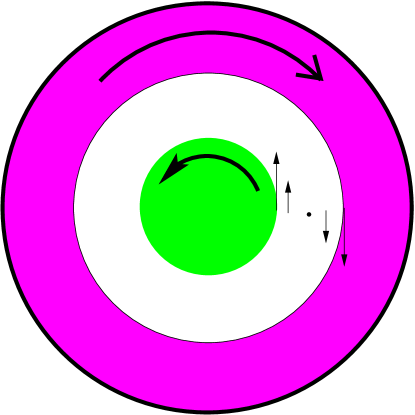
Now shrink the inner body to be the central rotating body and imagine the outer body to be the rest of the heavy universe. It is unreasonable to suppose that the qualitative description of inertial drag changes during the shrinking process and therefore, in the final metric, the central body will induce coherent inertial drag.
Now appeal to the same dimensional considerations as used in the passage quoted from MTW (above) to deduce the weak Sciama principle. Let the rotating body be labelled and have mass and angular velocity . For simplicity, consider a point on the equatorial plane of the rotating body at distance from the centre. It is a commonsense assumption that the dragging effect at is proportional to and, being a pure rotation of the local inertial frame, has dimension where means “time”. (Notice that there is no sensible meaning to the centre of rotation for this effect. Two rotations which have the same angular velocity but different centres differ by a uniform linear motion and inertial frames are only defined up to uniform linear motion.) Now in relativity time, mass and distance all have the same dimension. Thus is dimensionless and the only sensible formula for the induced inertial drag is , possibly normalised (note in passing that normalising constants such as are dimensionless and do not affect this argument).
Go further with this thought experiment. Assume now that the universe is spatially with the heavy inner rotating body at the origin. And imagine that the outer body is the outside of a sphere of radius say and is in fact at rest. Now let tend to infinity and, as it does so, control the mass of the outer body to keep its inertial effect near the inner body constant. In the limit, the outer body is replaced by an asymptotically flat metric near infinity and then, outside the inner body, is a metric which is stationary (the whole construction was stationary) axially-symmetric and asymptotically flat at infinity. Assume now that the theory being considered is in fact EGR. Then this metric must coincide with the Kerr metric which is well-known to be the unique metric satisfying Einstein’s equations for a vacuum with these properties. Equally well-known, the inertial drag effects of the Kerr metric drop off like . Thus this metric, constructed using the thought experiment, continuity and dimensional arguments, does not satisfy Einstein’s equations; or rather, to be very precise, if it is assumed that the space constructed is a vacuum outside the hypothesised masses, then the metric does not satisfy Einstein’s equations.
One may wonder why the dimensional argument does not equally apply to the Kerr metric. This is because the Kerr metric has a well-defined angular momentum but no well-defined angular velocity. Thus the inertial drag effect of the Kerr metric must be proportional to angular momentum NOT to mass times angular velocity. But angular momentum has dimension and to get a drag effect of dimension a formula of the type is needed where is angular momentum.
It is worth at this point recapping why angular momentum is the wrong measure for inertial effects. This is a simple consequence of the working hypothesis that linear motion has no inertial effect. Angular momentum can be altered by adding a linear motion. Angular velocity cannot be so altered.
2.8 Adding Sciama’s principle to EGR
At this point the story seems to have run into an impasse. Assuming the universe obeys standard relativity (EGR) then the version of Mach’s principle that is needed does not hold. Inertial drag drops off as in EGR and not .
There are two sensible ways out of this impasse.
(1)\quaThe revolutionary approach is to abandon EGR and build a new theory which satisfies Sciama’s principle.
(2)\quaThe conservative approach is to continue to use EGR but add a hypothesis within EGR that implies Sciama’s principle. As seen above, this is impossible assuming the space between bodies is a vacuum, so this approach entails hypothesing that space near a rotating body is not a vacuum and the thought experiment conducted above is impossible because the space between the rotating bodies is not a vacuum.
This book adopts the conservative approach. Apart from avoiding the non-trivial problem of finding a theory to replace EGR, this approach has one great technical advantage: it provides a mechanism for Mach’s principle (at least as it applies to rotation) which does not run into causal problems.
The hypothesis added to EGR is that any rotating body disturbs the local space-time by dragging inertial frames near it coherently by an amount proportional to the rotating mass times its angular velocity, with the influence dropping off asymptotically with where is distance from the centre of gravity of the rotating mass and is constant. The precise formula is given in the next chapter, where there is also an interpretation in terms of the metric.
In a vacuum, EGR does not have this inertial drag effect. The Kerr metric which is the only rotationally symmetric vacuum metric flat at infinity and valid in EGR has a drag effect dropping off much faster than this (asymptotically with ). So the hypothesis amounts to assuming that a rotating mass has a non-zero effect on the stress-energy tensor near it – in other words stops the space near it being a true vacuum. It also gives a natural way to understand how inertial drag propagates: the disturbance to the local vacuum is akin to a gravity wave and propagates at the speed of light. Furthermore reading back from the rest of the universe, the local background inertial frame is created by the rest of the universe by a similar propagation effect from all the rest of the matter. Thus the hypothesis gives a natural causal framework for Mach’s principle. An example of this causal framework working in practice would be the case where a rotating body undergoes a sudden change (eg breaking up) which changes the inertial drag field that it causes. This makes a disturbance in the local space-time (a sort of gravity wave) which propagates at the speed of light with no causal problems.
Another consequence is that a rotating body interacts directly with surrounding matter and indeed energy can be extracted in a similar way to the Penrose effect which extracts energy from the Kerr metric. This implies that the rotation will eventually radiate away. This is an extremely small effect for ordinary rotating bodies and only becomes significant for rotating black holes where the energy radiating away fuels the surrounding dynamic as will be seen in the next few chapters. The effect of this can be seen graphically in the spiral structure of full-size galaxies, eg the so called Whirlpool galaxy, \fullreffig:more_gals, left.
Superficially the change to vacuum that the new hypothesis entails may seem like an alternative formulation of “dark matter” but it is in fact quite different. The dark matter hypothesis amounts to assuming the existence of inert matter, which has no effect other than gravitational attraction, and cannot otherwise be detected. It is an incident hypothesis in the sense that it contains nothing more than what is needed to correct the rotation curve; it is a “fudge factor”, designed to correct a shortfall. The inertial drag hypothesis on the other hand amounts to assuming a new effect of a rotating body on the field outside it. It is justified by Mach’s principle which, as has been seen, is philosophically compelling and must be embodied in any theory that seeks to accurately describe reality. Thus it is a necessary hypothesis in the sense that it needs to made, independently of the rotation curve, in order to encode the necessary Mach principle. The inertial drag field that is assumed to exist can be detected directly by its effect on inertial frames so it has an existence independent of the rotation curve that it serendipitously also predicts.
In EGR a rotating mass does in fact have an effect on the field outside the body, but this is confined to the skew-symmetric part of the field (the Weyl tensor, or trace-free part of the curvature). So the new hypothesis implies that a rotating body also affects the other part, the Ricci curvature. Einstein’s equations for a vacuum are equivalent to the vanishing of the Ricci curvature (see \fullrefsec:Eequns). Thus, if the Ricci curvature is nonzero, then the field is not an Einstein vacuum.
2.9 Sciama’s principle and black holes
Applying Sciama’s principle to black holes entails assuming that a black hole has a well-defined angular velocity as well as a well-defined angular momentum. Equivalently a black hole has an effective radius, , related to angular momentum and angular velocity by
| (2.6) |
For a black hole the fiction is that the actual radius is zero (total gravitational collapse) and hence angular velocity is not determined. So this assumption is equivalent to replacing conventional theory by the more sensible assumption that, in the collapse to a black hole, matter reaches a small but non-zero size.
2.10 Coda
Sciama’s initiative, to base a dynamical theory on Mach’s principle as formulated in Sciama’s principle, has never been followed up and this approach to dynamics remains dormant. One of the aims of this book is to reawaken this approach. Sciama did return to the topic of Mach’s principle in [SWG]. However this paper abandons Sciama’s principle and formulates Mach’s principle in one of its weakest forms, namely that all phenomena have their origin in some material source or boundary condition. Moreover the theory exposited in [SWG] is EGR which as has been seen is incompatible with even the weak Sciama principle.
Chapter 3 The rotation curve
The rotation curve of a galaxy with an equatorial plane (for example a spiral galaxy has its spiral arms lying roughly in such a plane) is the plot of tangential velocity against distance from the centre for a particle (star or similar) moving in the equatorial plane. In practice it is not possible to observe one star, but rather the general motion of all stars (or other radiating matter) in the equatorial plane. This makes the observed nature of rotation curves all the more striking. Typically the curve (of tangential velocity against distance from the centre) comprises two approximately straight lines with a short transition region. The first line passes through the origin, in other words rotation near the centre has constant angular velocity (plate-like rotation); the second is horizontal, in other words the tangential velocity is asymptotically constant, see \fullreffig:modbeg (right) below. Furthermore, observations show that the horizontal straight line section of the rotation curve extends far outside the limits of the main visible parts of galaxies and the actual velocity is constant within less than an order of magnitude over all galaxies observed (typically between 100 and 300km/s) see \fullreffig:rotsSR.
Galactic rotation curves are so characteristic (and simple to describe) that there must be some strong structural reason for them. They are very far indeed from the curve obtained with a standard Keplerian model of rotation under any reasonable mass distribution. In a Keplerian model, suppose that the mass within a radius of the centre is then equating centrifugal force with gravitational attraction gives
where is tangential velocity and is Newton’s gravitational constant (taken to be 1 in natural units). Thus if is asymptotically constant then is asymptotically equal to a constant times and tends to infinity with .
Nevertheless, in spite of the huge mass needed, a Keplerian model is exactly what is assumed in current cosmological theory. To square the circle, current theory hypothesises the existence of a huge amount of matter. Since this matter is not observed, it is called called “dark”. It needs to be distributed in precisely the right way to make Keplerian rotation fit the rotation curve. This is extremely implausible for several reasons. Firstly it has just bben seen that the quantity of dark matter required is huge and tends to infinity with the radius of fit, which as mentioned above appears to be unbounded. Secondly it is unreasonable to suppose that exactly the right distribution of dark matter happened (by condensation) for every galaxy and thirdly, the final arrangement with most of the matter on the outside is dynamically unstable. For stability in a rotating system (such as the solar system or Saturn’s discs) there must be a strong central mass to hold it together. Failing this the system will tend to condense into smaller systems. Finally despite the best efforts expended in the search, nor hair nor hide of dark matter has been found to date.
This chapter presents a solution to these problems using a quite different point of view. The suggestion made here is that the centre of a typical galaxy contains a huge rotating body (probably a black hole) and that the inertial drag effects coming from this rotating mass are responsible for the observed rotation curves.
There is strong evidence that the masses of galaxies exceed the mass of the visible parts by some orders of magnitude. This goes back to Zwicky 1933 [Zwicky] who used the virial theorem to estimate the mass of galaxies in the Coma Berenices cluster and discovered that the mass exceeds luminosity mass by a factor of about . In current cosmological theory, this missing matter is identified with the invisible “dark matter” needed to make Keplerian motion fit the rotation curve. In the solution presented here, this extra matter is concentrated in the heavy rotating centre which controls the dynamics by inertial drag effects.
Assume that there is a standard background space (Minkowski or Schwarzschild space) and use an approximation to this background. Sciama’s principle as discussed in \fullrefsec:Sciama implies that the central rotating mass creates an inertial drag field dropping off like , which causes inertial frames to rotate with respect to the background. With this assumption, it is not hard to solve the equations to find the tangential velocity in an equatorial orbit as a function of (distance from the centre), and every equatorial orbit has the salient feature of observed rotation curves, namely a horizontal asymptote. This asymptote is the same for all equatorial orbits and hence any average over many orbits will also have this asymptote and this explains the observed rotation curve.
This provides strong evidence for the (weak) Sciama principle with inertial drag drop off asymptotically at as promised at the end of \fullrefsubsec:weakSp.
3.1 The weak Sciama principle
Sciama’s principle (\fullrefsubsec:Sp) implies that the rotation of the local inertial frame (IF) is the sum
where the sum is taken over all (accessible) masses in the universe where is at distance and rotating with angular velocity and the sum is suitably normalised .
For the purposes of this work, only the weak version is needed: (\fullrefsubsec:weakSp).
Weak Sciama Principle (WSP)\quaA mass at distance from rotating with angular velocity contributes a rotation of to the inertial frame at where is constant.
In the main application will be the (heavy) centre of a galaxy, but the analysis applies to any axially-symmetric rotating body which does not need to be assumed to be heavy.
To fix notation, consider a central mass at the origin in –space which is rotating in the right-hand sense about the –axis (ie counter-clockwise when viewed from above) with angular velocity . Assume a flat background space-time, away from , with sufficient fixed masses at large distances to establish a non-rotating IF near the origin, if the effect of is ignored. Let be a point in the equatorial plane (the –plane) at distance from the origin. The rotation of the inertial frame at is given by adding the contribution from to the contribution from the distant masses. Because is near a large mass, it makes sense to normalise the sum as in equation 2.3. This is equivalent to using a weighted sum, in other words the inertial frame at is rotating coherently with the rotation of by the average of weighted and zero (for the distant fixed masses) weighted say. Further normalise the weighting so that (which is the same as replacing by ) which leaves just one constant to be determined by experiment or theory. The nett effect is a rotation of
| (3.1) |
Note\quaIf the full Sciama principle is assumed and that (equation 2.2), which as was seen has some observational evidence to support it, then and are both 1 and and . However the choice of is not relevant to the arguments presented in this or subsequent chapters. Nothing that is proved depends on knowing the exact relationship between and .
3.2 The dynamical effect of the inertial drag field
The key to the rotation curve is to understand the way in which the inertial drag field affects the dynamics of particles moving near the origin. For simplicity work in the equatorial plane. Assume that the IF at (at distance from the origin) is rotating with respect to the background with angular velocity counter-clockwise. When computing rotation curves, the formula for just found (3.1) will be used but for the present discussion it is just as easy to assume a general function. The IF at can be identified with the background space, but it is important to remember that it is rotating. As remarked in \fullrefsubsec:weakSp there is no sensible meaning to the centre of rotation for an inertial frame. Two rotations which have the same angular velocity but different centres differ by a uniform linear motion and inertial frames are only defined up to uniform linear motion. Thus it can be assumed for simplicity that all the rotations have centre at the origin. Then the IFs can be pictured as layered transparent sheets, each comprising the same point-set but with each one rotating with a different angular velocity about the origin. Each sheet corresponds to a particuar value of . It is necessary to be very clear about the nature of motion in one of these frames. A particle moving with a frame (ie one stationary in that frame) has no inertial velocity and its velocity is called rotational. In general if a particle has velocity (measured in the background space) then
where its rotational velocity is the velocity due to rotation of the local inertial frame and is its inertial velocity which is the same as its velocity measured in the local inertial frame. Note that directed along the tangent.
The reader might find \fullreffig:IFs helpful at this point.

Inertial velocity correlates with the usual Newtonian concepts of centrifugal force and conservation of angular momentum.
As a particle moves in the equatorial plane it moves between the sheets so that a rotation about the origin which is rotational in one sheet becomes partly inertial in a nearby sheet. For definiteness, suppose that is a decreasing function of and consider a particle moving away from the origin and at the same time rotating counter-clockwise about the origin. The particle will appear to be being rotated by the sheet that it is in and this causes a tangential acceleration. This acceleration is called the slingshot effect because of the analogy with the familiar effect of releasing an object swinging on a string. But at the same time the particle is moving to a sheet where the rotation due to inertial drag is decreased and hence part of the tangential velocity becomes inertial and is affected by conservation of angular momentum which tends to decrease the angular velocity. These two effects balance each other out in the limit and this explains the flat asymptotic behaviour. Below this is proved analytically, but first, here is a metrical interpretation of the hypothesised inertial drag effect being used.
3.3 A metrical interpretation of inertial drag
Define an inertial drag metric by adding a variable rotation factor to a spherically-symmetric metric. The primary metrics of interest are obtained from the flat (Minkowski) metric and the Schwarzschild metric, but the proof of the rotation curve applies to any metric of this type. The inertial drag metric based on the Schwarzschild metric is likely to be close to the metric that will eventually be chosen if the conservative approach (cf \fullrefsubsec:Add) is generally adopted and serves to motivate the search for this metric.
Furthermore, as will be seen in the next chapter, a model for quasars based on the Schwarzschild metric successfully explains a good deal of the observations of these strange objects and this strongly suggests that this metric is a real reflection of reality at least in particular cases.
The most general spherically-symmetric metric can be written in the form:
| (3.2) |
where and are positive functions of and on a suitable domain. Here is time, is “distance from the centre” (but see the note below) and , the standard metric on the unit 2–sphere , is an abbreviation for . Orient the 2–sphere so that the –axis passes through it at the north pole where . The –plane (pasing through the origin and perpendicular to the –axis) is the equatorial plane where are polar coordinates. The Schwarzschild–de Sitter metric is the case
with and constants. By Birkhoff’s theorem (cf \fullrefsec:Birk) this is the only case where the metric satisfies Einstein’s vacuum equations with cosmological constant in some region. In this case the metric is necessarily static in this region. The special cases and give the Minkowski and Schwarzschild metrics respectively.
Note\quaIt is important to observe that is a coordinate which is not precisely the same as distance in the metric. It is chosen so that the sphere of symmetry at coordinate has area . Distance measured in the metric along a radius near this sphere is not the same as change in the coordinate (this only happens if takes the value 1 near the point under consideration).
The inertial drag metric is formed by adding a variable rotation about the –axis. This is done by replacing by . The metric is no longer diagonal
| (3.3) |
where .
If is constant this is the same metric viewed through rotating glasses, but the whole point is to allow to vary. Starting with the Schwarzschild–de Sitter metric and making this substitution with variable , gives a metric which no longer satisfies Einstein’s vacuum equations: indeed the change made is the metrical embodiment of the hypothesised inertial drag field. It is not hard to see that the inertial frame at a point rotates about a line parallel to the –axis with angular velocity the value of at that point. This is clear if is constant and in general, provided is continuous, it follows from the locality of inertial frames. So to fit with inertial drag as formulated in (3.1) it is necessary to set (at least in the –plane). However it is easy to work with a general function and specialise when needed. The orbits of particles moving on geodesics in the equatorial plane will now be investigatied and, provided decreases like as , the orbits will be found to fit observed rotation curves.
The reader might find \fullreffig:metric helpful for visualising geodesics in the inertial drag metric and understanding the inertial drag effects. It shows geodesics on a typical cylinder const.
2pt
\pinlabel [b] ¡2pt,0pt¿ at 103 202
\pinlabel [l] ¡2pt,0pt¿ at 233 108
\endlabellist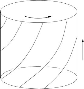
3.4 Conservation of angular momentum
The discussion continues with the analytic derivation of the rotation curve (the relation between and ) for the orbit of a particle in the equatorial plane moving with total velocity , which has tangential component (perpendicular to the line through the origin). Recall from the discussion in \fullrefsec:ideffects above that there are two opposing effects at work: the slingshot effect, which tends to increase with and conservation of angular momentum which tends to decrease it. These two effects are calculated together. The proof works in any inertial drag metric, where the particle moves along a geodesic. (The special case of flat Minkowski space with inertial drag effects was motivated in \fullrefsec:ideffects.)
The derivation starts with a proof of conservation of angular momentum, which is a property of any system with a central force (or space-time geometry which simulates a central force). It is not restricted to Newtonian physics. The proof is adapted from Newton’s proof of the equal area law for planetary orbits (which law is exactly the same as conservation of angular momemtum). For the time being ignore (or set it equal to zero).
2pt
\pinlabel [r] ¡0pt,0pt¿ at 19 233
\pinlabel [br] ¡0pt,0pt¿ at 36 275
\pinlabel [l] ¡0pt,0pt¿ at 105 275
\pinlabel [l] ¡0pt,0pt¿ at 104 202
\pinlabel [t] ¡0pt,0pt¿ at 35 0
\pinlabel [b] ¡0pt,0pt¿ at 67 275
\pinlabel [t] ¡0pt,-1pt¿ at 56 219
\pinlabel [r] ¡1pt,0pt¿ at 33 121
\pinlabel [l] ¡1pt,0pt¿ at 71 111
\pinlabel [lb] ¡0pt,0pt¿ at 65 242
\endlabellist
The idea is to replace the central force by a series of central impulses at equally spaced (small) intervals of time. Consider \fullreffig:CAM. At a particular time the particle (of small unit mass) is at and has just received a central impulse resulting in velocity . Its tangential velocity at is . One small interval of time later the particle is at and receives another central impulse (along the line ) which does not change its tangential velocity . But the triangle can be regarded as having base and height or base and height hence
| (3.4) |
in other words the angular momentum at is the same as that at .
To obtain the result for an arbitrary continuous central force, take the limit of a sequence of central impulses. Note the proof does not use any property of the central force other than that it acts towards the centre. Nor does it assume that represents a genuine distance in the metric under consideration. All that is needed is that Euclidean geometry correctly describes the relationship between and distances perpendicular to radii near and which is precisely how was chosen.
3.5 The fundamental relation
Now reinstate . Note that “force” in the model is a property of local space-time geometry. In the case that is constant, the inertial frame (rotating with ) is the same as the unrotated case and in this frame the force is central. Therefore by locality it is central in the general case in the inertial frame. Therefore the proof just given makes sense in the inertial frame at , in other words rotating with angular velocity , though, as will be seen, in the limit the same result is obtained if it is assumed that the frame is rotating with angular velocity . To find the required relationship between and write for the full tangential velocity at and at . Since the frame is rotating at , and . Write , , and .
Since (equation 3.4), substituting for and simplifying gives
| (3.5) |
But
and substituting for in (3.5) gives
which gives
It is now possible to replace by to first order (as forecast) and going to the limit yields the fundamental relation between and :
| (3.6) |
The fundamental relation can be understand intuitively as follows. The slingshot effect intuitively produces an acceleration . On the other hand is the “inertial” tangential velocity (corrected for rotation of the local inertial frame) and therefore conservation of angular momentum produces a deceleration in of or an acceleration . Adding the two effects gives the relation.
3.6 Solving to find rotation curves
Given as a function of , (3.6) can be solved to give as a function of . Rewrite it as
The LHS is and the general solution is
| (3.7) |
It is now clear that any prescribed differentiable rotation curve can be obtained by making a suitable choice of continuous .
Of interest here are solutions which, like observed rotation curves, are asymptotically constant and inspecting (3.7) this happens precisely when is asymptotically equal to for some and this happens precisely when is asymptotically equal to . This proves the following result.
Theorem.
The equatorial geodesics in the inertial drag metric (3.3) have tangential velocity asymptotically equal to constant if and only if is asymptotically equal to where .
3.7 The basic model
Now specialise to the case which gives the value of inertial drag formulated in (3.1). The constant in the theorem is no longer needed and it is reused.
From (3.7)
| (3.8) |
where is a constant depending on initial conditions. For a particle ejected from the centre with for small, , and for general initial conditions there is a contribution to which does not affect the behaviour for large . For the solution with there are two asymptotes. For small, and the curve is roughly a straight line through the origin. And for large the curve approaches the horizontal line . A rough graph is given in \fullreffig:modbeg (left) where . The similarity with a typical rotation curve, \fullreffig:modbeg (right), is obvious. Note that no attempt has been made here to use meaningful units on the left. See \fullreffig:rotsmod below for curves from the model using sensible units.
2 [r] at 14 457
\pinlabel1 [r] at 14 247
\pinlabel10 [t] at 130 17
\pinlabel20 [t] at 252 17
\pinlabel30 [t] at 364 17
\pinlabel40 [t] at 463 17
\endlabellist\cl
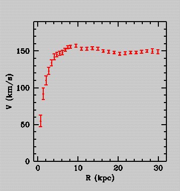
There are other shapes for rotation curves; see [SR] for a survey. All agree on the characteristic horizontal straight line. \fullreffig:rotsSR is reproduced from [SR] and gives a good selection of rotation curves superimposed. In \fullreffig:rotsmod is a selection of rotation curves again superimposed, sketched using Mathematica\fnoteThe notebook Rots.nb used to draw this figure can be collected from [Nb] and the values of the parameters used read off. and the model given here. The different curves correspond to choices of and . The similarity is again obvious. The units used differ. In the model given here natural units are used so that a velocity of .001 is 300km/s and a distance of 45,000 is 15Kpc approx.
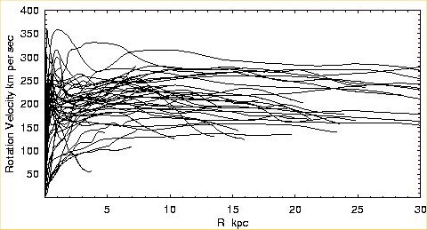
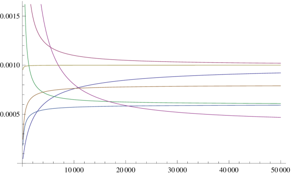
It is worth commenting that the observed rotation curve for a galaxy is not the same as the rotation curve for one particle, which is what has been modelled here. When observing a galaxy, many particles are observed at once and what is seen is a rotation curve made from several different rotation curves for particles, which may be close but not identical. So it is expected that the observed rotation curves have variations from the modelled rotation curve for one particle, which is exactly what is seen in Figures 3.4 (right) and 3.5.
The next chapter is devoted to the other main application of inertial drag, namely quasars. Then in \fullrefsec:spiral_struc the analysis given here will be extended to find equations for orbits in general (not just for the tangential velocity) and, using a hypothesised central generator, the spiral arm structure will be modelled as well. The basic idea is that the central mass accretes a belt of matter which develops instability and explodes feeding the roots of the arms. Stars are formed by condension in the arms and move outwards as they develop. Thus a typical star is on a long outward orbit and the rotation curve observed for stars in a spiral arm is formed of many such similar orbits. But this full picture is not necessary to explain the observed rotation curves, since the tangential velocity for all orbits has the same horizontal asymptote. \fullrefsec:spiral_struc is more specific about the size of the central mass in a galaxy. These vary from to solar masses with the range to corresponding to so-called “active galaxies” and the range to to full-size spiral galaxies. The central masses for the curves in \fullreffig:rotsmod vary from to solar masses and it is useful to know that a mass of 1 in natural units is solar masses.
3.8 Postscript
As remarked earlier, the effect described in this chapter is independent of mass. However for rotating bodies of small mass the effect is unobservably small. For example the sun has 3km, assuming , and days. Thus the asymptotic tangential velocity is 6km per 4 days or .06 km per hour.
Chapter 4 Quasars
quasar\nlkweıza:, kweısa:,\nlnoun Astronomy\nlnoun: quasar; plural noun: quasars
a massive and extremely remote celestial object, emitting exceptionally large amounts of energy, which typically has a starlike image in a telescope. It has been suggested that quasars contain massive black holes and may represent a stage in the evolution of some galaxies.
Origin\nl1960s: contraction of quasi-stellar.
Google dictionary definition (October 2017)
Quasars were first observed in the 1960’s. Through a telescope they appear to be stars but they exhibit strange features not shared by ordinary stars. They have spectra which often appear to be hugely redshifted and they vary irregularly with time scales that range from hours to months. Early in the study of quasars a heated controversy raged about these huge redshifts. Are they cosmological due to the expansion of the universe? or are they gravitational due to the near presence of a massive object (eg a black hole)? The cosmological explanation implies that quasars with large redshifts are extremely distant objects with truly phenomenal power outputs which are very hard to explain. By constrast the gravitational explanation allows the possibility that they are modest size objects, not too distant and with easily modelled power outputs. As can be seen from the Google definition, the cosmological explanation is the currently accepted one. This is despite some incontrovertible evidence in the form of observations of Halton Arp and others [Arp, Getal] that quasars are often closely associated with galaxies with the redshift for the quasars significantly higher than that for the associated galaxies, a striking example of which is reproduced in \fullreffig:NGC7603.
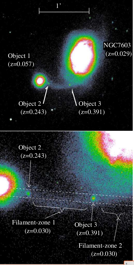
This example contains two Arp quasars (objects 2 and 3) strongly associated with a galaxy (and companion) both of lower redshift. Lopez Corredoira and Gutierrez [LCG] report and mag for the main galaxy, NGC 7603 and comment: “A fact that attracted attention is its proximity to NGC 7603B (Object 1 hereafter), a spiral galaxy with higher redshift , moreover a filament can be observed connecting both galaxies. They also found two objects superimposed on the filament with redshifts and for the objects closest to and farthest from NGC 7603, Objects 3 and 2, respectively. –magnitudes corrected for extinction (due to the filament) are respectively and .”
It is commonsense that the alignments seen in \fullreffig:NGC7603 are not due to chance and there are many similar such in Arp and other’s observations [Arp, Getal]. Objects 2 and 3 have cosmological redshift around (for the filament) and the remainder must be instrinsic (presumably gravitational). As often happens when a consensus view is challenged by direct evidence, the evidence is ignored and the challenger discredited. Arp was sidelined by the mainstream cosmological community and denied observation time on the big telescopes. If this book can serve to rehabilitate Arp’s reputation (unfortunately posthumous) it will have been worth writing.
The purpose of this chapter is to explain how the same inertial drag phenomenon used in the last chapter to model rotation curves can be used to restore a sensible explanation for these observations and to establish a simple model for quasars with modest power output that explains all the observations.
4.1 Angular momentum and inertial drag
As explained in the introduction, the strongest argument supporting the current consensus view (that redshift in quasars is cosmological) comes from a consideration of angular momentum. Assume that a quasar contains a large central mass (presumed to be a black hole) and that its energy production is due to accretion from the surrounding medium. Particles fall into the gravitational well of the central mass and the gravitational energy is released by interaction between different infalling particles. Now given a small but very heavy object, a particle approaching with a small tangential velocity will have its tangential velocity magnified by conservation of angular momentum and there will be a radius of closest approach. It is very unlikely to actually fall into the central gravitational well, and the same thing happens for the full flow of infalling matter from the surrounding medium, which will typically have a nonzero angular momentum around the black hole. (See the Michel quote in \fullrefsec:intro.) This gives an obstruction to accretion, which was found not long after quasars were discovered, and led to the subject being dominated by the theory of accretion discs.
But now assume that the central mass is rotating and that the infalling particle is in the equatorial plane. Take inertial drag effects into consideration. From (3.7) the angular momentum per unit mass of the particle can be read as . This is the apparent angular momentum (as calculated by a distant viewer). To find the true angular momentum (ie as measured in the local inertial frame) replace by , which entails subtracting from , so the true angular momentum (per unit mass) is
| (4.1) |
By suitable choice of the integration constant, there are solutions with low angular velocity (either true or apparent) for small and significant angular velocity for larger and it follows that the effect of the inertial drag is that the rotating body can absorb angular momentum. And notice that this holds for almost any dynamical theory, in particular general relativity. (It also works with almost any nontrivial function .)
Now if angular momentum can be nullified by central rotation, then it does not force the existence of an accretion disc and a simple spherically-symmetric model for accretion can be used. Here is another description of the effect being used here which gives further information. The formula for (equation 3.1) implies that IFs near the origin rotate at roughly the same rate, in other words all fit with a plate-like rotation. If the speed of this rotation is the same as the effective rotation of the infalling matter then the latter rotation will be “rotational” (due to the rotation of the IF) and not “inertial”. Thus conservation of angular momentum (which acts only on inertial velocity) will not change it and the inflow will be radial in the local inertial frame. Moreover there is a feedback effect working in favour of this. If the incoming matter has excess angular momentum, then it will tend to contribute to the central rotation which therefore changes to increase the inertial drag effect until the two balance again. Conversely, if there is a shortfall, the black hole will slow down. In other words, once locked on the ambient conditions that allow the black hole to accrete, there is a mechanism for maintaining that state.
At this point recall that given a black hole with angular velocity and angular momentum then (2.6) where is the effective radius of the black hole, assumed to be small but not zero. Thus a very small change in angular momentum corresponds to a reasonable change in the angular velocity. This makes the locking effect described above more responsive and effective.
If the incoming matter has angular momentum about a different axis than the rotation axis for the black hole, then a similar feedback effect will cause the black hole rotation axis to change into alignment with axis for the incoming matter.
The conclusion is that the angular momentum obstruction for accretion can effectively be ignored and a spherically symmetric accretion model used. A suitable model based on the Schwarzschild metric is studied in joint work with Robert MacKay and Rosemberg Toala Enriques [BHQR]. In this model gravitational redshift can take arbitrary values
| (4.2) |
where is the black hole mass in solar masses, is density of the ambient gasplasma in number of particles per cubic metre (assumed to be Hydrogen atoms or protons) and is temperature in degrees Kelvin. is an absorption factor which can be taken to be (ie ingore the factor in square brackets). The full technical details of the model (hereafter called the “three-author model”) are given in \fullrefapp:3author, where equation (4.2) is proved. Notice one important point about this equation. The mass of the black hole appear inverted so that (other parameters being equal) redshift decreases with black hole mass. This was observed directly by Arp and caused him to invent some fantasy physics to explain it because he was not aware of the considerations discussed here.
Also in the appendix are many worked examples including NGC7603 and associated objects. One particular quasar is worth mentioning here because of the (in fact false, as will be seen) importance that it has for the Milky Way, namely Sagittarius . This quasar is regarded as problematic by the mainstream quasar community because its level of radiation is 8 orders of magnitude below the Eddington limit. It is suggested here that this is due to a very high redshift, , which causes the power to be attenuated by the square of this, namely . Full details and supporting evidence from the luminosity graph can be found at the end of \fullrefsec:data.
This chapter finishes with an outline of this three-author model and discussion of evidence and previous work on quasars. Note that this chapter and the related appendix use MKS units and not the natural units used in other chapters.
4.2 Outline of the three-author model
As remarked earlier this model for black hole radiation (aka quasar radiation) is spherically-symmetric, fully relativistic and based on the Schwarzschild metric. There are fully relativistic Schwarzschild black hole models to be found in the literature, for example the models of Flammang, Thorne and Zytkow [FTZ] quoted by Meier [meier, page 490]. But the significance of these models, and in particular their redshift, has been ignored, presumably because of the angular momentum obstruction discussed above. Thus the excellent fit with observations that is found has been overlooked.
In the three-author model, black holes radiate by converting the gravitational energy of incoming matter into radiation and, since only a fraction of the available energy is radiated back out, they accrete mass and grow over time. There will be a good deal more to say about this growth in later parts of the book. It is highly suggestive of a life-form.
The basic set-up considered is a black hole floating in a gas of Hydrogen atoms (the medium), which might be partially ionised (ie form a plasma), with the radiation coming from accretion energy. Matter falls into the black hole and is accelerated. Interaction of particles near the black hole changes the “kinetic energy” (KE) of the incoming particles into thermal energy of the medium and increases the degree of ionisation. The thermal energy is partially radiant and causes the perceived black hole radiation.
Kinetic energy is not a relativistic concept as it depends on a particular choice of inertial frame in which to measure it. It is for this reason that it has been placed in inverted commas. Nevertheless, it is a very useful intuitive concept for understanding the process being described here.
The following simple considerations suggest that most of the KE of the infalling matter is converted into heat and available to be radiated outwards. A typical particle is very unlikely to have purely radial velocity. A small tangential velocity corresponds to a specific angular momentum. As the particle approaches the black hole, conservation of angular momentum causes the tangential velocity to increase. Thus the KE increase due to gravitational acceleration goes largely into energy of tangential motion. Different particles are likely to have different directions of tangential motion and the resulting melée of particles all moving on roughly tangential orbits with varying directions is the main vehicle for interchange of KE into heat and hence radiation. Very little energy remains in the radial motion, to be absorbed by the black hole as particles finally fall into it. Thus the overall radial motion of particles is slow. In terms of the models of [FTZ], the “breeze solutions” for radial flow [meier, Figure 12.2, page 489] are being used. Far away from the black hole, where density is close to ambient density, and therefore low, this process converts angular momentum into radial motion with little loss of energy and serves to allow the plasma to settle into the inner regions, where the density is higher and the particle interactions generate heat and radiation.
4.3 Three important spheres
For simplicity of exposition now assume that the medium is a Hydrogen plasma and the heavy particles are therefore protons. This is true in the higher temperature parts of the model, for example once the Eddington sphere is reached, see below. But there is no material difference if the medium is in fact a partially ionised Hydrogen gas.
Observations of quasars often show the presence of other atomic material in the radiation zone so that this simplifying assumption may need revision at a later stage.
There are three important spheres. The outermost sphere is the Bondi sphere of radius defined by equating the average velocity of protons in the medium with the escape velocity at radius . Here is the black hole mass, is the gravitational constant, is Boltzmann’s constant, is temperature and is the mass of a proton.
The significance of the Bondi sphere is that protons in the medium are trapped (on average) inside this sphere because they have KE too small to escape the gravitational field of the black hole. The mass of matter per unit time trapped in this way is called the accretion rate and can be calculated as
| (4.3) |
where is the density of the medium (number of protons per unit volume).
Details for these calculations are given in \fullrefsec:Bondi.
Proceeding inwards, the next important sphere is the Eddington sphere of radius which is defined by equating outward radiation pressure on the protons in the medium with inward gravitational attraction from the black hole. More precisely, the outward radiation pressure acts on the electrons in the medium which in turn pull the protons by electrical forces. This is the same consideration as used to define the Eddington limit for stars and this is why the same name has been used. At the Eddington sphere the gravitational pull on an incoming proton is balanced by the outwards radiation pressure (mediated by electrons) and, assuming the radiation pressure is just a little bigger, the acceleration of the incoming proton is replaced by deceleration and the KE of infall is absorbed by the medium and available to feed the radiation. It is a definite hypothesis that there is an Eddington sphere, but the final model that is constructed using this hypothesis does fit facts pretty well, and this justifies it.
It is helpful to think of the Eddington sphere as a transition barrier akin to the photosphere of a star. Indeed the Eddington radius is also the radius at which photons get trapped in the medium and for this reason is also known as the trapping radius. This can be seen by thinking of the forces that define it the other way round. The incoming matter flow exerts a force on the outward radiation and when these two are in balance, the outward radiation is stopped and photons are trapped.
Thus at the Eddington sphere two things are happening: the infalling protons are stopped and their KE released into the general pool of thermal energy and the outward flow of radiation is also stopped. Thus radiation from the black hole is generated by activity in the close neighbourhood of the Eddington sphere and this is the place where redshift of the outward radiation due to the gravitational pull of the black hole arises.
The region outside the Eddington sphere is optically thin whilst the region inside is optically thick. The radiation that is emitted comes from a narrow band near the Eddington sphere and which is all at roughly the same distance from the central black hole. This allows the radiation to exhibit a consistent redshift.
Precise formulae that determine the Eddington radius in terms of the other parameters are given in \fullrefsec:KE.
The final sphere is the familiar Schwarzschild sphere or event horizon of radius where is the black hole mass.
The region between the Schwarzschild and Eddington spheres is called the active region and the region between the Bondi sphere and the Eddington sphere, the outer region. A simplifying assumption is made that nearly all the KE that powers the black hole is released in the active region. This means that any KE turned into heat by particle interaction in the outer region is ignored. This is justified by the fact that this region has low density, close to the ambient density, so that most particle interactions are between particles sufficiently far apart to conserve kinetic energy. It is useful to think of this region as a “settling region” where angular momentum is converted into radial motion, allowing the plasma to settle towards the active region. See also the discussion below equation (LABEL:eq:PreTrap) and in \fullrefsec:conc.
One other simplifying assumption is made: it is assumed that there is no significant increase in temperature near the Bondi sphere due to the black hole radiation, ie is the ambient temperature.
4.4 Previous work on quasars and gravitational redshift
This chapter finishes with a review of the historical reasons for abandoning the idea that quasars might have significant instrinsic (gravitational) redshift and why they do not apply to the model.
The principal reason (angular momentum) has already been fully explained. There are four main further reasons:
(1)\quaRedshift gradient (see the discussion in [fifty-years] on pages 3–4)
If redshift is due to a local mass affecting the region where radiation is generated, then the gravitational gradient from approach to the mass would spread out the redshift and result in very wide emission lines. This effect is called “redshift gradient”.
In the model, although the energy production takes place throughout the active region, the emitted radiation is generated only at (or near) the Eddington sphere which is all at the same distance from the central mass and subject to the same redshift. Thus the model has the observed property that emission lines are moderately narrow.
(2)\quaForbidden lines (cf Greenstein–Schmidt [G-S])
Many examples of black hole radiation show so-called forbidden lines, which can only be produced by gas or plasma at a fairly low density. The assumption that all the radiation is produced by a low density region leads to an implausibly large and heavy mass (see [G-S, page 1, para 2]).
In the three-author model, the region directly adjacent to the Eddington sphere is at roughly ambient density which is, in all examples that are examined in the appendix, low enough to support forbidden lines (more details on this will be given in \fullrefsec:calc). A narrow shell of low density near the Eddington sphere is excited by the radiation produced at the sphere and produces radiation in turn. It is here that forbidden transitions take place and result in the observed forbidden lines.
(3)\quaMass and variability problems (cf Greenstein–Schmidt [G-S], Hoyle–Fowler [H-F])
The mass problem is a rider on the forbidden line problem but also applies to attempts at models for gravitational redshift without significant redshift gradient. As remarked above, assuming that all the radiation is produced by a low density region leads to an implausibly large and heavy mass. The same thing happens if one tries to produce a region with sufficient local gravitational field to provide a base for the radiation production, without redshift gradient, as for example in Hoyle and Fowler [H-F]. This problem is compounded by the fact that quasars typically vary with time scales from days to years. For variability over a short timescale, a small production region is needed (significantly smaller than the distance that light travels in one period).
It is worth remarking in passing that this problem is unresolved by the current assumption that all quasar redshift is cosmological. This implies that quasars are huge and very distant so that special (and unnatural) mechanisms are invoked to explain variability.
In the three-author model, the size of the radiation producing region is small enough. The black hole sizes that fit observations are in the range to solar masses. For quasars with significant intrinsic redshift, the radius of the Eddington sphere has the same order of magnitude as the Schwarzschild radius, and for solar masses this is metres or light seconds or about 20 light minutes. Thus the natural mechanism for variability, namely orbiting clouds or more solid bodies causing periodic changes in observed luminosity, fits the facts perfectly.
It is also worth observing here that there is a quite remarkable paper of M R S Hawkins [H], which proves an apparently paradoxical result, namely that a certain sample of quasars exhibits redshift without time dilation. The paradox arises from the fact that redshift and time dilation are identical in general relativity. Indeed they are identical in any theory based on space-time geometry. What Hawkins actually finds is a sample of quasars with varying redshift for which the macroscopic variation in light intensity does not correlate with the redshift. The resolution of the paradox is that the mechanism that produces the redshift and the mechanism which causes the variability are not subject to the same gravitational field. This is precisely how the model works. The redshift is caused by the central black hole and the variability is caused by orbiting clouds etc, much further out, and in a region of lower redshift. For more detail on the Hawkins paper and its meaning see \fullrefsec:hawk. Properly understood, the paper proves conclusively that quasars typically have intrinsic redshift.
(4)\quaStatistical surveys
Stockton [S] is widely cited as a proof that quasar redshift is cosmological. He takes a carefully selected sample of quasars and searches for nearby galaxies within a small angular distance and at close redshift. Out of a chosen sample of 27 quasars, he finds a total of 8 which have nearby galaxies with close redshifts. He assumes that all these quasars have significant intrinsic redshifts and are therefore not actually near their associated galaxies. He then calculates the probability of one of these coincidences occurring by chance at about 1/30, and concludes that the probability of this number of coincidences all occurring by chance is about 1.5 in a million.
The conclusion he draws is that all quasar redshift is cosmological.
The fallacy is obvious from this summary. It may well be that many of the quasars in the survey do not have significant intrinsic redshift and therefore some of these coincidences are not chance events. As can be seen from equation (4.2) the three-author model allows the gravitational redshift of a quasar to vary from near zero to as large as you please. Roughly speaking, redshift is small (orders of magnitude smaller than 1) if the mass is big or the medium is dense and cold. Conversely, with a small mass and a hot thin medium, the redshift can be several orders of magnitude greater than 1. There is a natural progression for a quasar, as it accretes mass and grows heavier, to start with a very high gravitational redshift and gradually evolve towards a very low one. Without a sensible population model for quasars, it is difficult to comment on the number of coincidences that Stockton finds, but it is highly plausible that heavy quasars (with low gravitational redshift and central masses of say to solar masses) gravitate towards galactic clusters and therefore have nearby galaxies at a similar cosmological redshift. This would provide a natural framework for the Stockton survey within the model.
Stockton does discuss the possibility that quasars may have both small and large intrinsic redshifts (see [S, page 753, right]), but the discussion is marred by assuming that the two classes must be unrelated objects. The three-author model has a natural progression between the two classes.
There is a more modern survey by Tang and Zhang [T-Z] which also claims to prove that all quasar redshift is cosmological. But examining the paper carefully, what is actually proved is that some particular models for quasar birth and subsequent movement are incompatible with observations. To comment properly on this paper a good population model for quasars would again be needed. But it is worth briefly mentioning that at least one of their models (ejection at m/s from active galaxies with a lifespan of years) does fit facts fairly well, see [T-Z, figure 1, page 5]. The ejection velocity is implausibly large, but the lifespan could easily be 50 times larger allowing for a plausible ejection velocity of say m/s and a better fit with the data.
Finally, there is another interesting argument given by Wright [LAF] “proving” that quasar redshift is all cosmological from details of the spectra. This is the Lyman-alpha-forest argument. The observations he cites give useful information about the outer region. This, and the fallacy in the argument, will be discussed near the end of \fullrefapp:3author in \fullrefsec:conc.
The story continues in \fullrefapp:3author where full technical details of the three-author model and the fit with data can be found.
But to finish this chapter here are some comments on quasar growth. It has been seen that quasars grow by accretion and lose their intrinsic redshift (as observed by Arp, but explained using non-standard physics). If, as Arp suggests, they are ejected from mature galaxies, then there is a natural way to think of them as young galaxies. As they grow and gain mass, they will take on more and more features of active galaxies and finally develop into mature spiral galaxies (discussed in the next chapter). As a highly speculative example, the grouping of four objects (two galaxies and two quasars) seen in \fullreffig:NGC7603 could be a “family” group: two adults and two children. Indeed the quasar–galaxy spectrum has all the appearances of forming the dominant lifeform for the universe. This topic is taken up again in sections 5.2 and LABEL:sec:lords.
Chapter 5 Spiral structure
The chapter combines ideas from the last two chapters to give a complete description of the dynamics of spiral galaxies.
5.1 Introduction
Spiral galaxies (Figures 5.1, 5.3, LABEL:fig:more_gals) are surely the most beautiful objects in the universe and it comes as a shock to find that there is no proper theory for their structure in current cosmology.
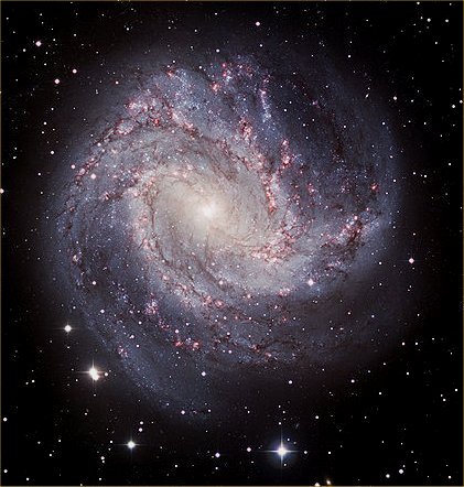
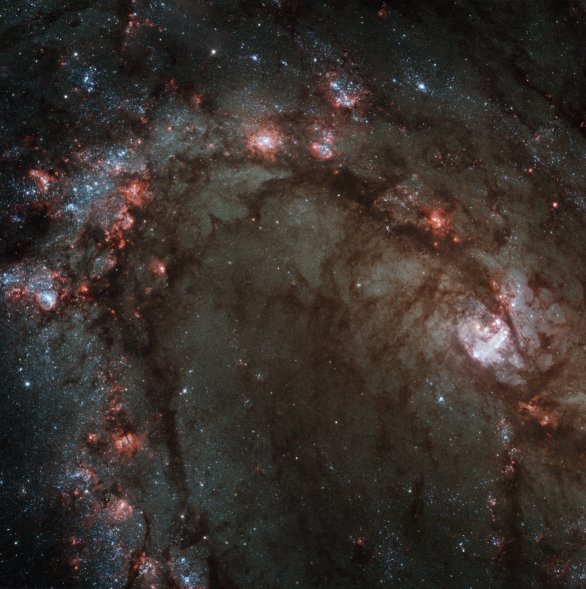
The main problem arises from the assumption that stars move on roughly circular orbits. In order for a spiral structure to be maintained stably over several revolutions, with all stars moving on circular orbits, it is necessary for tangential velocity to be roughly proportional to distance from the centre which means that the rotation curve is far from the one observed, \fullreffig:rot-stand (left). This problem is known as the “winding dilemma”. In order to solve this problem conventional cosmology proposes that the spiral arms are not real but virtual. It proposes that they are in fact “standing waves” or “density waves”, \fullreffig:rot-stand (right). Although this theory gives plausible spirals, the nature of the arms in real galaxies, \fullreffig:galaxies (right) or \fullreffig:more_gals (left) does not fit it at all. Real arms are composed of a spiral curve of intense star producing regions and associated high luminosity short-life stars, see for example the close up of M83 from the Hubble site \fullreffig:M83 right. There is no trace of the orbits that are supposed to form the density wave outside the actual spiral arm. To be a little fairer to the standing wave theory, there is a rider to the theory which suggests that a shock-wave effect causes short-life stars to appear as the standing wave moves. Indeed it is clear from any galactic picture that the main luminosity of typical spiral arms comes from high luminosity short-life stars, but the short-life stars produced by a shock wave would last long enough to blur the arms and the pictures are quite clear: no such blurring occurs. Moreover, this model begs the question of where the continuous supply of pre-stellar material comes from to support this creation process.
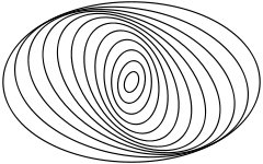
In this chapter a quite different solution to this problem is proposed. The idea is, instead of assuming that stars move on roughly circular orbits, to assume that they move outwards along the arms as they rotate around the centre. Thus the familiar spiral structure is like the visible spiral structure in a Catherine wheel, the arms being maintained by stars moving along them, and there is no need for any special pleading to explain the observed structure. Moreover, the motion can be modelled and the stable spiral structure demonstrated . The model has one crucial feature in common with the standing wave theory in its shock-wave version: the visible spiral structure does consist mainly of short-life stars and star-producing regions and this common feature is crucial for accurate modelling because it allows for elapsed time along the arms of about years which fits the models constructed here. More details on this are given in \fullrefsec:math. The problem of supply of pre-stellar material is solved in the model by continuous replenishment from the centre of the galaxy.
Two assumptions are needed, the first of which was anticipated in \fullrefsec:rot_curve to explain the observed rotation curve, namely that the centre of a normal spiral galaxy such as the Milky Way contains a hypermassive black hole, of mass solar masses or more. The second assumption is that this black hole is ringed by an accretion torus of a very precise type, which is called the generator or belt and which is responsible for generating the streams of material which feed and maintain the spiral arms. The belt is an example of the accretion structures hypothesised for the nuclei of “active” galaxies (for which central super-massive black holes, of to solar masses, have been directly observed) and used to explain their observed radiation. “Active” has been placed in quotation marks because of one of the main theses of this book, that all galaxies are active: the activity of a spiral galaxy is responsible for its spiral structure; indeed there is no distinction between active galaxies and “normal” spiral galaxies. The real difference is that the central black hole in a normal galaxy is masked from view by the matter which is trapped in accretion structures near it, the most prominent of which is the central bulge. The spectrum of black hole based objects will be discussed further in \fullrefsec:obs.
The assumption of a hypermassive central black hole in a spiral galaxy directly contradicts current beliefs of the nature of Sagittarius and this problem together with other observational matters will be dealt with in the next chapter (\fullrefsec:astar). Very briefly, Sgr and the stars in close orbit around it form an old globular cluster near the end of its life with most of the matter condensed into the central black hole. It is not at the centre of the galaxy but merely roughly on line to the centre and it is about half-way from the sun to the real galactic centre which is invisible to us.
As remarked above, in the new model for galactic dynamics proposed here, young stars in a galaxy are moving outwards as well as around the centre. This general outward movement has not been observed, although there are some old observations of Oort, Kerr and Westerhout [OKW] which show outward movement in gas clouds but which are generally misinterpreted (see \fullrefsec:21). Indeed, early observations of Lindblad, using Shapley’s maps of globular cluster, suggested that stars in the neighbourhood of the sun move on circular orbits (see [BM, page 16]) and this has created an idée fixe that all stars in galaxies move on roughly circular orbits with any contrary observations explained away on an ad hoc basis. In the model proposed here, motion of stars is far from Keplerian, being strongly controlled by inertial drag effects from the (rotating) centre. The result is that the outward progress takes a very long time—commensurate with the lifetime of a star—and hence the outward velocity, far out from the centre where the Sun lies, is rather smaller than (about one tenth of) the observed rotational velocity. Thus the new model is consistent with the Lindblad observations. For more detail here, see the analytic models constructed in \fullrefsec:math.
The general picture which emerges is of a structure stable over an extremely long timescale (at least years) with stars born and aging on their outward journey from the centre and returning to the centre to be recycled with new matter to form new solar systems. The tentative suggestion is that galaxies have a natural lifetime of perhaps years with the universe considerably older than this. The consequences of these suggestions for cosmology as a whole will be discussed in the next chapter; here note that the theory of galactic dynamics presented in this chapter does not depend on this timescale. Indeed it could at a pinch be consistent with the current standard model for the universe as a whole starting with the big bang. But the author’s opinion is that the big bang theory is a serious mistake. For more detail here see \fullrefsec:bb .
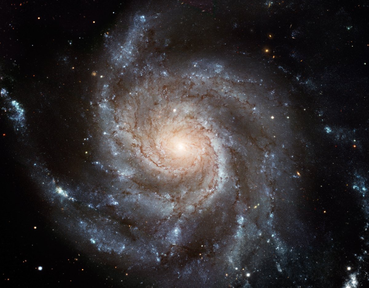
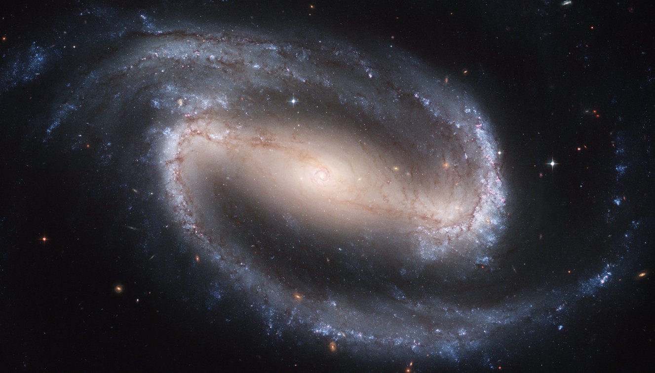
5.2 The generator
The full dynamics of spiral galaxies will be developed in the next and following sections, but first here is an outline of the proposed generator for the spiral arms. The story is part of the main story of the book, namely the quasar–galaxy spectrum, which will be taken up again in \fullrefsec:spec and following sections. The keys to understanding the generator are the familiar ones: angular momentum and inertial drag. Previous chapters have covered the start of the story: inertial drag effects allow a black hole (aka quasar) to cancel out the angular momentum obstruction to accretion and feed on the surrounding medium and hence grow in size. As it grows the mass increases and its intrinsic (aka gravitational) redshift decreases. For a very small quasar such as Sgr of mass solar masses, the intrinsic redshift can be very large (in this case a figure of is indicated by observations), but for a larger quasar (of size say solar masses) is more typical, but there is a huge variation, see the tables at the end of \fullrefsec:data.
As the mass grows and the instrinsic redshift decreases, the simple spherical accretion model, described in \fullrefsec:quasars and \fullrefapp:3author, breaks down because the accretion rate is too great for smooth accretion to take place. The outer settling region develops instabilities; there is evidence for this starting in the so called “Lyman-alpha forest” (see the end of \fullrefsec:data). The flow accumulates near the Eddington sphere choking the inflow. A rotating toroidal accretion structure (the belt), similar to the conventional theory, forms \fullreffig:belt (left).
Notice that as the material in orbit around the black hole grows in mass and extent, it increasingly masks the central black hole and the virial theorem typically used to estimate this mass becomes less useful. This point in the spectrum is where “active” galaxies (of mass in the range – solar masses) start.
The quasar starts to produce explosive outflow (jets) and to morph into an active galaxy. The angular momentum locking effect, described in \fullrefsubsec:locking_effect, is now no longer stable because the jets carry away angular momentum and cause the whole system to rotate in the opposite direction to the rotation of the belt. So the central black hole is rotating to the left (say) and a surrounding belt is rotating to the right \fullreffig:belt (right). (Note that throughout this chapter anticlockwise or positive (positive value of ) is used in all illustrations for the main rotation of the central body; the belt has negative (clockwise) rotation.) This implies that the angular momentum in the inertial frames is augmented by the inertial drag effects described earlier and the effective energy in the belt similarly augmented. Thus energy is being fed into the belt structure directly from the black hole itself. There are also two other sources of energy for the belt: accretion energy as for any quasar and energy (heat) caused by interference due to inertial drag between layers: a sort of “friction” effect. With all this energy going into the belt, it becomes extremely hot and a plasma of quarks forms nearest the centre, condensing into a normal plasma of ionised H and He nuclei, with a trace of Li, further out. Conditions here are similar to those hypothesised to have occurred just after the big bang and the resulting mix of elements is the same. The energy results in explosions causing the jets mentioned already. As mass increases the jets become massive and permanently established and manifest themselves as the familiar spiral arms of the galaxy as explained below.
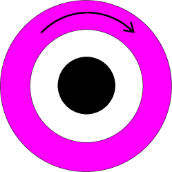
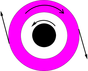
At the same time there is a build-up of matter trapped near the central black hole, visible as the familiar bulge, which totally masks the black hole, and the fiction that the central black hole of the Milky Way could be only solar masses is not obviously wrong (though it is completely incompatible with the dynamics presented in this chapter).
Once the central black hole starts rotating, the inertial drag effects calculated in Sections 3.2 and LABEL:sec:dyn come into play and, further out, matter ejected from the centre starts to rotate with the hole and against the rotation of the belt. Matter is lost from the outer regions and, if ejected from the centre fairly slowly so that the inertial drag effect dominates, carries away angular momentum of the opposite sign, \fullreffig:arms.
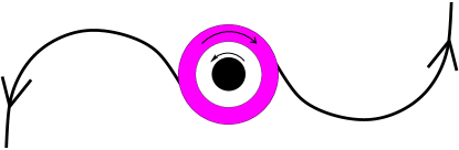
There is a stable situation in which the loss of angular momentum in both directions is in balance: highly energetic particles ejected from the belt are not strongly affected by inertial drag effects and carry away clockwise angular momentum; less energetic particles are affected and carry away anticlockwise angular momentum. This balancing effect is why there is strong stability in the limiting tangential velocity, in other words why rotation velocity is roughly constant over all galaxies observed, \fullreffig:rotsSR. Note that \fullreffig:arms shows orbits not arms. It should be compared with \fullreffig:loose left. Inertial drag causes the roots of the arms to appear to precess clockwise and the snapshot of orbits that is seen has the familiar spiral form (as demonstrated in the Mathematica drawn figures in \fullrefsec:math).
Energy is lost from the black hole because of the matter ejected from the belt, but energy is recovered by matter falling into the active region near the black hole so that the whole structure is stable over an immense timescale. In the next chapter compatibility of this model with the timescale of the big bang is discussed. This global loss of energy implies that there is no further growth in general, indeed there is now steady loss due to radiation energy and matter lost to the system, to balance accretion.
The spiral arms form as follows. The explosions from the belt mentioned above are the mechanism which feeds the spiral arms. These do not occur in random places: most normal galaxies have a pronounced bilateral symmetry with two main opposing arms (eg Figures 5.1, 5.3 and LABEL:fig:more_gals). There is no intrinsic reason for this to happen, but it is a stable situation. Once two arms have formed, then the gravitational pull of these arms will form bulges at the roots of the arms and encourage explosions there to feed the arms. The bilateral symmetry arises because the bulges are tidal bulges, caused by the pull of the nearby spriral arms, and tidal bulges always have bilateral symmetry. This tendency to bilateral structure is weak and looking at a gallery of galaxies many examples where it fails to form or where other weak arms have formed as well as the two main arms can be found.
Notice that ejection from the belt is generally in the direction of the belt rotation, which is opposite to the direction of the black hole rotation and this as will be explained later is why the roots of the arms generally have a noticeable offset (see the galaxy examples referred to above). To be precise, there is a constant in the model which sets the tangential velocity at the root of the arms, and with this set negative, the arms are offset, cf \fullrefsec:math.
How the structure fits with detailed observations of our galaxy, the Milky Way, and other nearby galaxies is explained in the next chapter, and more detail on the composition of the arms and of the corresponding stellar population distribution is given. Here it only needs to be noted that the arms are fed by a stream of gasplasma (comprising H, He and a trace of Li) ejected from the belt which condenses into stars which then form the visible spiral arms.
5.3 The full dynamic
The construction of the model that will explain spiral structure starts here. The first step is to extend the analysis of \fullrefsec:rot_curve to obtain a full model for orbits in the galactic plane and not just a formula for the rotation curve of such an orbit. The analysis applies to any rotating mass, but the results are only significant for truly enormous masses such as the hypothesised central mass in a galaxy.
Equation 3.8 (in \fullrefsec:rot_curve) gave a formula for the tangential velocity in an orbit. What is needed is a formula for the radial velocity (again in terms of ) and these two will describe the full dynamic in the equatorial plane, which can then be used to plot orbits.
Intuitively there are two radial “forces” on a particle: a centripetal force because of the attraction of the massive centre and a centrifugal force caused by rotation in excess of that due to inertial drag. Thus a formula for radial acceleration of the following form is expected
| (5.1) |
where and is the effective central “force” at radius , per unit mass. The same notation as in \fullrefsec:rot_curve is used here and in particular is the inertial drag at radius .
This will be proved in a similar way to the proof of conservation of angular momentum given in \fullrefsec:rot_curve, using a geometrical argument which is valid in the inertial drag metric.
2pt
\pinlabel [r] ¡0pt,0pt¿ at 19 233
\pinlabel [br] ¡0pt,0pt¿ at 36 275
\pinlabel [l] ¡0pt,0pt¿ at 105 275
\pinlabel [l] ¡0pt,0pt¿ at 104 202
\pinlabel [t] ¡0pt,0pt¿ at 35 0
\pinlabel [b] ¡0pt,0pt¿ at 67 275
\pinlabel [t] ¡0pt,-1pt¿ at 56 219
\pinlabel [r] ¡1pt,0pt¿ at 33 121
\pinlabel [l] ¡1pt,0pt¿ at 71 111
\pinlabel [l] ¡0pt,0pt¿ at 104 244
\pinlabel [r] ¡1pt,2pt¿ at 25 252
\pinlabel [lb] ¡0pt,0pt¿ at 65 242
\endlabellist