The scaling of the X–ray variability with black hole mass in AGN

Abstract

The relation between the $2-10$ keV, long term, excess variance and AGN black hole mass is considered in this work. A significant anti-correlation is found between these two quantities in the sense that the excess variance decreases with increasing black hole mass. This anti-correlation is consistent with the hypothesis that the $2-10$ keV power spectrum in AGN follows a power law of slope $-2$ at high frequencies. It then flattens to a slope of $-1$ below a break frequency, $\nu_{hfb}$, until a second break frequency, $\nu_{lfb}$, below which it flattens to a slope of zero. The ratio $\nu_{hfb}$/$\nu_{lfb}$ is equal to $10-30$, similar to the ratio of the respective frequencies in Cyg X-1. The power spectrum amplitude in the (frequency $\times$ power) space does not depend on black hole mass. Instead it is roughly equal to $0.02$ in all objects. The high frequency break decreases with increasing black hole mass according to the relation $\nu_{hfb}$$=1.5\times 10^{-6}/$(M/$10^{7}$ M_⊙) Hz, in the case of “classical” Seyfert 1 galaxies. The excess variance of NGC 4051, a Narrow Line Seyfert 1 object, is larger than what is expected for its black hole mass and X–ray luminosity. This can be explained if its $\nu_{hfb}$ is 20 times larger than the value expected in the case of a “classical” Seyfert 1 with the same black hole mass. Finally, the excess variance vs X–ray luminosity correlation is a byproduct of the excess variance vs black hole mass correlation, with AGN accreting at $\sim 0.1-0.15$ the Eddington limit. These results are consistent with recent results from the power spectral analysis of AGN. However, as they are based on data from a few objects only, further investigation is necessary to confirm that there is indeed a “universal” power spectrum shape in AGN (in the sense that the value of the power spectrum parameters of most AGN will be distributed around the “canonical” slope, and amplitude values listed above). One way to achieve this is to determine the excess variance vs black hole relation more accurately, using data from many more objects. This will be possible in the near future, since it is easier to measure the excess variance of archival light curves than to estimate their power spectrum. The excess variance vs black hole relation can therefore play an important role in the study of the X–ray variability scaling with black hole mass in AGN.

1 Introduction

Since the beginning of the active galactic nuclei (AGN) X–ray variability studies it was noticed that more luminous sources show “slower” variations. Barr & Mushotzky (1986) were the first to show that the “two-folding” time-scale (i.e. the time-scale for the emitted flux to change by a factor of two) was faster in lower luminosity objects. Later, Lawrence & Papadakis (1993) and Green et al. (1993), using the results from the power spectral density function (PSD) analysis of the EXOSAT “long looks”, showed that the PSD amplitude at a given frequency decreases with increasing source luminosity. Nandra et al. (1997) and George et al. (2000), using the so called “excess variance” ($\sigma^{2}_{rms}$, i.e. the variance of a light curve normalised by its mean squared after correcting for the experimental noise) found an anti-correlation between excess variance and source luminosity. Similar results were also presented by Leighly (1999) and Turner et al. (1999), who also found that a particular group of AGN, the so called “Narrow Line Seyfert 1” (NLS1) galaxies, show systematically larger variability amplitude when compared to the same luminosity “classical” AGN (i.e. Seyferts with predominantly broad permitted lines, BLS1s). Further progress in the study of the longer-term X–ray variability has been afforded by RXTE, which has allowed systematic observations over time-scales longer than before (i.e. months, years). Markowitz & Edelson (2001), using 300 day long RXTE light curves of nine Seyfert galaxies, estimated their excess variance and found a significant anti-correlation between $\sigma^{2}_{rms}$ and source luminosity even on these long time-scales.

Most of the previous studies have examined the dependence of the “variability amplitude” on the source luminosity. However, during the last few years, the mass of the central black hole has been estimated for many AGN (see e.g. Woo & Urry 2002 for a recent compilation of AGN black hole mass estimates). It is therefore possible to investigate the dependence of the variability amplitude on the black hole mass (M_BH), a fundamental property of AGN. Recent studies that have followed this approach, have shown that there exists a significant anti-correlation between $\sigma^{2}_{rms}$ and M_BH, using ASCA light curves of BLS1s and NLS1s (Lu & Yu, 2001; Bian & Zao, 2003).

The primary goal of the present work is to investigate the relation between excess variance and M_BH using the $\sigma^{2}_{rms}$ data of Markowitz & Edelson (2001), together with the recent $\sigma^{2}_{rms}$ measurement of a radio-quiet quasar, namely PG 0804+761 (Papadakis, Reig, & Nandra, 2003). Markowitz & Edelson (2001) have already shown that $\sigma^{2}_{rms}$ is strongly anti-correlated with the source luminosity. It is important though to see if there exists a correlation between $\sigma^{2}_{rms}$ and M_BH as well. In this way, one can relate the observed X–ray variations to the physical system itself, since M_BH is an important physical parameter of AGN. Based on the fact that the integral of the PSD is equal to the variance of a light curve, the $\sigma^{2}_{rms}$–M_BH relation is used in order to examine the intrinsic shape of the PSD in AGN, and how this correlates with M_BH. Obviously, a single $\sigma^{2}_{rms}$ value can correspond to different power spectral forms. As a result, the $\sigma^{2}_{rms}$–M_BH relation cannot provide us with a unique answer as to what is the intrinsic shape of PSD in AGN, and how this might correlate/change with M_BH. However, assuming a certain PSD shape, the study of the $\sigma^{2}_{rms}$–M_BH relation can be a powerful tool in assessing the reality of the assumed PSD shape.

In this work, the $\sigma^{2}_{rms}$–M_BH relation is used in order to examine the recent results from the power spectrum analysis of RXTE, XMM-Newton and ASCA light curves of AGN (e.g. Uttley, McHardy,& Papadakis, 2002; Markowitz et al., 2003). These results have increased significantly our knowledge of the intrinsic PSD shape of AGN. However, high quality PSD estimation is currently possible for a few objects only, due to the lack of a large number of data sets that meet the necessary requirements (i.e. high signal-to-noise, long, well sampled light curves). The results presented in this work are also based on the use of a small number of objects, which have high quality, long term $\sigma^{2}_{rms}$ measurements. However, although the number of objects with accurate PSD estimation may not increase significantly in the near future, the study of the $\sigma^{2}_{rms}$–M_BH relation can be extended soon to incorporate the use of $\sigma^{2}_{rms}$ measurements from a large number of objects. For example, the are numerous AGN observations with RXTE and ASCA, which last typically for $\sim 1$ day (assuming a $\sim 30-40$ ksec exposure time). Although the PSD estimation is difficult with these light curves, the measurement of their $\sigma^{2}_{rms}$ is easier. Taking also into account the wealth of the new data that are currently provided by XMM-Newton, and CHANDRA, it will be possible to define the $\sigma^{2}_{rms}$–M_BH relation more accurately in the near future. Consequently, the $\sigma^{2}_{rms}$–M_BH relation will probably play an important role in the study of the X–ray variability scaling with M_BH in AGN.

2 The dependence of long term variability amplitude on BH mass

Markowitz & Edelson (2001) have calculated the excess variance for nine Seyfert galaxies using 300 day long, RXTE (PCA), $2-10$ keV light curves with a uniform $5$ day sampling. Recently, Papadakis et al. (2003) calculated the excess variance of PG 0804+761 using a year long, RXTE (PCA), $2-10$ keV light curve with a $3$ day sampling. The sampling and duration of the quasar light curve is similar to the respective properties of the Seyfert galaxy light curves of Markowitz & Edelson. Therefore the quasar $\sigma^{2}_{rms}$ measurement can be used together with the Seyfert values. The $\sigma^{2}_{rms}$ values, together with M_BH estimates, are listed in Table 1. In most cases, the M_BH estimates are taken from Kaspi et al. (2000), and they correspond to the mean of their “rms FWHM” and “mean FWHM” estimates. All objects with a $\sigma^{2}_{rms}$ estimate are BLS1s except from NGC 4051 and MCG 6-30-15, which are classified as NLS1s.

Table 1: The excess variance ($\sigma^{2}_{rms}$), PSD break frequency ($\nu_{hfb}$) and black hole mass (M_BH) estimates of the objects studied in this work. The objects are ranked by their M_BH.

Name	Type	$\sigma^{2}_{rms}$	$\nu_{hfb}$	BHMass
		$(\times 10^{-2})$	($\times 10^{-6}$ Hz)	($\times 10^{7}$ M${}_{\odot})$
Akn 120	BLS1	$3.7\pm 0.7$	$-$	$18.6(1)$
PG0804	BLS1	$2.1\pm 0.4$	$-$	$17.6(1)$
3C120	BLS1	$3.9\pm 0.8$	$-$	$13.5(2)$
NGC 5548	BLS1	$5.4\pm 1.1$	$0.6^{+1.9}_{-0.5}(1)$	$10.9(1)$
Fairal 9 (F9)	BLS1	$4.4\pm 0.9$	$0.4^{+0.23}_{-0.24}(1)$	$8.2(1)$
NGC 5506	NLS1	$-$	$51.2^{+49}_{-50.8}(2)$	$8.8^{*}$
NGC 3516	BLS1	$8.7\pm 1.7$	$2.0^{+3}_{-1}(1)$	$1.7(3)$
NGC 4151	BLS1	$10.3\pm 2.1$	$1.3^{+1.9}_{-1.0}(1)$	$1.4(1)$
NGC 3783	BLS1	$5.3\pm 1.1$	$4.0^{+6.0}_{-1.5}(1)$	$1.0(1)$
Mrk766	NLS1	$-$	$500^{+300}_{-300}(4)$	$0.35(2)$
MCG-6-30-15	NLS1	$8.0\pm 1.6$	$100^{+100}_{-60}(3)$	$0.1(4)$
NGC 4051	NLS1	$20\pm 4.0$	$800^{+400}_{-300}(5)$	$0.05(5)$
NGC 4395	BLS1	$-$	$320^{+320}_{-160}(6)$	$0.0066(6)$
Ark564	NLS1	$-$	$1700^{+600}_{-900}(7)$	$<0.8(7)$

Column 2 lists the object type (BLS1 or NLS1). Note that NGC 5506 was recently classified as NLS1 (Nagar et al., 2002). All $\sigma^{2}_{rms}$ estimates in Col. (3) are taken from Markowitz & Edelson (2001), except from PG 0804+761 which is taken from Papadakis et al. (2003). The numbers in parenthesis in Col. (4) correspond to the references for $\nu_{hfb}$ as follows: (1) Markowitz et al. (2003), (2) Uttley et al. (2002), (3) Vaughan et al. (2003), (4) Vaughan & Fabian (2003), (5) McHardy et al. (2003), (6) Shih et al. (2003), (7) Papadakis et al. (2002). Note that the $\nu_{hfb}$ values of NGC 5548 and F9, together with their errors, are taken from Table 5 of Markowitz et al., while the respective estimate of NGC 3783 was taken from Section 4.3 of the same work. The numbers in parenthesis in Col. (5) correspond to the references for M_BH as follows: (1) Kaspi et al. (2000), (2) Woo & Urry (2002), (3) Onken et al. (2003), (4) Uttley et al. (2002), (5) Shemmer et al. (2003), (6) Filippenko & Ho (2003), (7) Collier et al. (2001). The BH mass for NGC 5006 is estimated as explained in the text. Note that the M_BH estimate of MCG 6-30-15 is rather uncertain (see discussion in Section 6.3 of Uttley et al., 2002.)

In order to compute the uncertainty of the $\sigma^{2}_{rms}$ estimates, the uncertainty of the PG 0804+761 $\sigma^{2}_{rms}$ measurement was estimated first, based on the PSD results of Papadakis et al. (2003). As $\sigma^{2}_{rms}$ is roughly equal to the PSD integral from the highest to the lowest sampled frequency, using the best-fitting parameter values from the power-law model fitting to the PSD, it is straightforward to compute the uncertainty of the PSD integral over the sampled frequencies, and hence $\sigma^{2}_{rms}$ itself. The result shows that [error($\sigma^{2}_{rms}$)/$\sigma^{2}_{rms}$]$\sim 0.2$. The uncertainty of the PSD integral depends mainly on the frequency range and frequency resolution of the PSD. These properties are determined by the number of points and the length of the light curve. Since all the $\sigma^{2}_{rms}$ values listed in Table 1 are estimated by light curves with almost identical length and number of points, the “signal-to-noise” ratio of the $\sigma^{2}_{rms}$ values should be $\sim 0.2$ in all cases. The $\sigma^{2}_{rms}$ errors listed in Table 1 are computed based on this assumption. As for the M_BH estimates, reverberation mapping and stellar velocity dispersion methods give reliable estimates within factors of a few (Woo & Urry, 2002). However, it is difficult to determine the actual error of all the individual M_BH estimates listed in Table 1. For that reason they will not be considered hereafter.

Figure 1: RXTE excess variance plotted as a function of M_BH. The solid line shows the best-fitting model in the case of a universal PSD with $\nu_{hfb}$ $\propto$ M_BH^-1. The long-dashed line shows the $\sigma^{2}_{rms}$ vs M_BH relation in the case when $\nu_{hfb}$ scales with M_BH with a normalisation 20 times larger than case of the model shown with the solid line. The short-dashed and dot-dashed lines show a model with two PSD break frequencies, $\nu_{hfb}$ and $\nu_{lfb}$, with $\nu_{lfb}$ being $10-30$ time smaller than $\nu_{hfb}$, respectively (see text for details).

Fig. 1 shows the $\sigma^{2}_{rms}$ vs M_BH plot. Clearly, there is a strong correlation between the two variables in the sense that that $\sigma^{2}_{rms}$ decreases with increasing M_BH. Computation of Kendal’s $\tau$ yields $-0.69$, which implies that the anti-correlation between $\sigma^{2}_{rms}$ and M_BH is highly significant (probability $>99.5\%$).

Let us suppose that the power spectrum, normalised to the mean squared, follows the form: $P(\nu)=A(\nu/\nu_{hfb})^{-1}$ Hz^-1, for $\nu<\nu_{hfb}$, and the form: $P(\nu)=A(\nu/\nu_{hfb})^{-2}$ Hz^-1, at higher frequencies ($A$ is the PSD value at $\nu=\nu_{hfb}$). Let us also suppose that the PSD “amplitude”, i.e. PSD_amp=$A\times\nu_{hfb}$, is constant and does not depend on M_BH, while $\nu_{hfb}$ is inversely proportional to the black hole mass, i.e. $\nu_{hfb}$$=C/$M₇ Hz, where M₇=M_BH/$10^{7}$M_⊙. Under these assumptions, one can find a unique relation between $\sigma^{2}_{rms}$ and M₇ using the fact that $\sigma^{2}_{rms}=\int_{\nu_{ls}}^{\infty}P(\nu)d\nu$, where $\nu_{ls}$ is the lowest frequency sampled ($=1/300$ days = $3.858\times 10^{-8}$ Hz, for the objects considered in this work). Note that, strictly speaking, the upper limit of the $\sigma^{2}_{rms}$ integral should be closer to $2\Delta T_{obs}$, where $\Delta T_{obs}\sim 1$ ksec is the length of the individual monitoring exposures, since variations on shorter time scales are smoothed out. In any case though, use of either limits does not affect the integral’s value almost at all.

The integral’s estimation depends on whether $\nu_{hfb}$ is higher or lower than $\nu_{ls}$. In the first case, one can show that:

$$\sigma^{2}_{rms}={\rm PSD_{amp}}\times[\ln(C/{\rm M}_{7})+18.07],$$ (1)

while in the second case, $\sigma^{2}_{rms}$ is given by the relation,

$$\sigma^{2}_{rms}={\rm PSD_{amp}}\times 2.592\times 10^{7}\times C/{\rm M}_{7}.$$ (2)

The data shown in Fig. 1 were fitted with the model given by equations (1) and (2), excluding the points which correspond to the two NLS1s. The best fitting model is also shown in Fig 1 (solid line). The best fitting model parameter values are PSD_amp$=0.017\pm 0.006$, and $C=1.7^{+3.9}_{-0.8}\times 10^{-6}$ Hz (errors correspond to the $68\%$ confidence for two interesting parameters, i.e. $\Delta\chi^{2}=\chi^{2}+2.3$). Although the model does not provide a statistically accepted fit to the data ($\chi^{2}=14.8/6$ dof), it describes rather well the overall trend of decreasing $\sigma^{2}_{rms}$ with increasing M_BH. The $\sigma^{2}_{rms}$ values of the two NLS1s (NGC 4051 and MCG 6-30-15), NGC 3783, and PG 0804+761 show the largest deviations from the best fitting model.

2.1 The possibility of a second frequency break in the PSDs

If there is a second PSD flattening to zero slope at a frequency $\nu_{lfb}$$<$$\nu_{hfb}$ (like the PSD of Galactic black hole candidates, GBHs, when at low/hard state), then $\sigma^{2}_{rms}$ is given by the following relation,

$$\sigma^{2}_{rms}={\rm PSD_{amp}}\times[2-\nu_{ls}/\nu_{lfb}+\ln(\nu_{hfb})-\ln(\nu_{lfb})],$$ (3)

in the case when $\nu_{lfb}$$>\nu_{ls}$. In the opposite case, $\sigma^{2}_{rms}$ is not affected by the presence of $\nu_{lfb}$  and equations (1), (2) still hold. The dashed and dot-dashed lines in Fig. 1 show a plot of equation (3) using the best fitting PSD_amp and $C$ values from the previous section, and assuming that $\nu_{hfb}$/$\nu_{lfb}$$=10-30$, respectively. This ratio is similar to the ratio of the respective break frequencies in the PSD of Cyg X-1 at low/hard state (Belloni & Hasinger, 1990). Equation (3) provides an acceptable fit to all data (except from NGC 4051): $\chi^{2}=10.7/7$ dof and $\chi^{2}=10.2/7$ in the case when $\nu_{hfb}$/$\nu_{lfb}$$=10-30$, respectively.

As Fig. 1 shows, the MCG 6-30-15 and NGC 3783 $\sigma^{2}_{rms}$ measurements are now consistent with the model defined by equation (3). In other words, their $\sigma^{2}_{rms}$ measurements suggest that there are two breaks in their PSD, both of which are higher than $\nu_{ls}$. Interestingly, the observed PSD of NGC 3783 does show two breaks, with $\nu_{hfb}$/$\nu_{lfb}$$\sim 20$ (Markowitz et al., 2003). However, only one break (which corresponds to the “$-2$ to $-1$” slope flattening) has been reported in the case of MCG 6-30-15. Uttley et al. (2002) and Vaughan, Fabian, & Nandra (2003), report $\nu_{hfb}$$\sim 5\times 10^{-5}$ Hz, and $\sim 1\times 10^{-4}$ Hz, respectively, with the two values being consistent within the errors. If indeed $\nu_{hfb}$ $\sim 5\times 10^{-5}-10^{-4}$ Hz, the present results suggest that the low frequency break should be located at a frequency $10-30$ times lower, i.e. at around $\sim 1-5\times 10^{-6}$ Hz. Such a break should be detected by Uttley et al. (2002), as their PSD extends to frequencies lower than $\sim 10^{-7}$ Hz. A combined long-term RXTE and short-term XMM-Newton PSD could resolve this issue.

2.2 The case of NGC 4051

NGC 4051 is the only source which deviates significantly from all model lines plotted in Fig. 1. This NLS1 is one of the most variable radio-quiet AGN. The discrepancy between the NGC 4051 $\sigma^{2}_{rms}$ estimate and the model defined by equation (3) (dashed and dot-dashed lines in Fig. 1) suggests that the PSD of this object should have just one frequency break at frequencies higher than $1/300$ days^-1. This is consistent with the results of McHardy et al. (2003). Using RXTE and XMM-Newton data, McHardy et al. detect a frequency break at $\sim 8\times 10^{-4}$ Hz (where the PSD changes slope from $-2$ to $-1$), but they do not observe any further flattening at lower frequencies down to $10^{-8}$ Hz. However, the NGC 4051 $\sigma^{2}_{rms}$ measurement does not agree with the best-fitting model defined by equations (1) and (2) (solid line in Fig. 1). This implies that either the PSD_ampof NGC 4051 is larger than in other AGN, or $\nu_{hfb}$ is higher than expected for its M_BH. According to the results of McHardy et al. (2003), PSD_amp$\sim 0.01$, which is smaller than the best fitting PSD_amp value of $0.017$. Therefore, the $\sigma^{2}_{rms}$ measurement of NGC 4051 can be consistent with equations (1) and (2) only if $C$ is increased. The long-dashed line in Fig. 1 shows a plot of the model defined by equations (1) and (2), using PSD_amp$=0.017$, and $C=20$ times larger than the best-fitting value reported in Section 2. The agreement now between the model and the NGC 4051 measurement is good.

2.3 The scaling of $\nu_{hfb}$ with M_BH

One of the results from the model fitting of the $\sigma^{2}_{rms}$–M_BH relation is that, under the assumption of a universal PSD shape in AGN, then $\nu_{hfb}$$\sim 1.7\times 10^{-6}/$M₇ Hz. It is interesting to see how this relation compares with the results from the power spectral analysis of recent observations in AGN. Table 1 lists the M_BH and $\nu_{hfb}$ estimates for all AGN where a “$-2$ to $-1$” frequency break has been detected recently, irrespective of whether the same object has a long term $\sigma^{2}_{rms}$ measurement or not. The M_BH of NGC 5506 was estimated using the stellar velocity dispersion measurement of 180 km/sec (Oliva et al., 1999), together with the M_BH – stellar velocity dispersion relation of Tremaine et al. (2002).

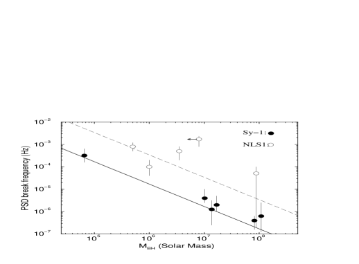
Figure 2: PSD Break frequency plotted as a function of M_BH. The solid line shows a plot of the $\nu_{bf}$$=C/M_{7}$ relation, with $C$ being equal to the value from the best model fitting of the $\sigma^{2}_{rms}$–M_BH relation. The dash line shows a plot of the same relation with $C$ being 20 times larger.

Fig. 2 shows a plot of $\nu_{hfb}$ as a function of M_BH. The solid line is not a plot of the best fitting model to the data. Instead, it shows a plot of the $\nu_{bf}=C/$M₇ relation, with $C=1.7\times 10^{-6}$ Hz (i.e. the value estimated from the best model fitting to the $\sigma^{2}_{rms}$ vs M_BH data in Section 2). The agreement between this line and the BLS1 data is very good. However, the NLS1s $\nu_{hfb}$ estimates lie consistently above the solid line. The dashed line in Fig. 2 shows a plot of the $\nu_{bf}=C/$M₇ with $C=20\times 1.7\times 10^{-6}$ Hz (i.e. the $C$ value which can explain the high $\sigma^{2}_{rms}$ measurement of NGC 4051, as discussed in Section 2.2). As Fig. 2 shows, the agreement between this line and the $\nu_{hfb}$ measurements of NLS1s is good. Therefore, both the large value of the $\sigma^{2}_{rms}$ measurement of NGC 4051 and the location of the NLS1 data in Fig. 2 suggest that, for the same M_BH, $\nu_{hfb}$ is $\sim$ 20 times higher in NLS1s than in BLS1s.

2.4 A universal PSD_amp value in AGN?

Another result from the study the $\sigma^{2}_{rms}$–M_BH relation is that PSD_amp should be $\sim 0.017$ in all AGN. It is not straightforward to compare this result with recent results from power spectral analysis of X–ray light curves, as in most cases the PSD normalisation is not reported. In the cases where the relevant information is listed, the estimated PSD_amp values are indeed close to 0.017. For example, using the results of Markowitz et al. (2003), one can find that: PSD_amp=0.021, 0.016, 0.012, 0.016, and 0.017 in the case of F9, NGC 5548, NGC 3783, NGC 3516, and NGC 4151, respectively. In the case of Cyg X-1, the Belloni & Hasinger (1990) data suggest that PSD_amp$=0.02\pm 0.002$. This is consistent, within the errors, with the value of 0.017. Interestingly, the existing data for NLS1s are systematically lower than 0.017. For example, Papadakis et al. (2002) and Vaughan & Fabian (2003) find PSD_amp$\sim 0.005$ and $\sim 0.01$ in the case of Ark 564 and Mrk 766, respectively. Furthermore, McHrady et al. (2003) find PSD_amp$\sim 0.01$ for NGC 4051. However, this value was estimated using a PSD model different than the “broken power-law model” used in the other cases. In fact, as Figure 17 in McHardy et al.(2003) shows clearly, the PSD_amp of NGC 4051 is probably as large as the PSD_amp of other BLS1s.

2.5 The accretion rate of AGN

Figure 3: The excess variance measurements plotted as a function of the X–ray ($2-10$ keV) luminosity. The dot-dashed line shows a plot of the expected $\sigma^{2}_{rms}$–$L_{X}$ relation using the results from the best model fitting of the $\sigma^{2}_{rms}$–M_BH relation (shown with the dot-dashed line in Fig. 1), and assuming that $L_{X}\propto$M_BH. The solid and dashed lines show plots of models defined to account for the high $\sigma^{2}_{rms}$ measurement of NGC 4051 (see text for details).

It is interesting to investigate if the $\sigma^{2}_{rms}$ vs $2-10$ keV X–ray luminosity ($L_{X}$) correlation of Markowitz & Edelson (2001) is in fact a byproduct of the $\sigma^{2}_{rms}$ vs M_BH correlation presented in this work. This is possible only if there exists a relation between M_BH and $L_{X}$, which is the same for all the objects. This implies that the accretion rate, when considered as a fraction of the Eddington limit, should be similar in all objects.

Fig. 3 shows the $\sigma^{2}_{rms}$–$L_{X}$ relation for the objects with $\sigma^{2}_{rms}$ measurements listed in Table 1, using the $L_{X}$ measurements of Markowitz et al. (2003) for F9, NGC 5548, NGC 3783, NGC 3516, and NGC 4151, Markowitz & Edelson (2001) for 3C120, Akn120, and MCG -6-30-15, McHardy et al. (2003) for NGC 4051, and the measurement of Papadakis et al. (2003) for PG 0804+761. The dot-dashed line in Fig. 3 shows a plot of a model, which is based on: (1) the best fitting “2 PSD breaks with $\nu_{lfb}$/$\nu_{hfb}$=30” model to the $\sigma^{2}_{rms}$–M_BH relation (the one shown with the dot-dashed line in Fig. 1), and (2) the relation $L_{X}=({\rm BH}_{\rm Mass}/{\rm M}_{\odot})\times 10^{35.8}$ ergs/sec. As Fig. 3 shows clearly, this line fits the data very well ($\chi^{2}=8.8/9$ dof), except from NGC 4051. Using the mean bolometric conversion factor of $L_{bol}\sim 27\times L_{X}$ of Padovani & Rafanelli (1988), the adopted relation between $L_{X}$ and M_BH implies that $L_{bol}=1.7\times 10^{37}({\rm BH}_{\rm Mass}/{\rm M}_{\odot})$ ergs/sec. Since $L_{\rm Edd}=1.25\times 10^{38}({\rm BH}_{\rm Mass}/{\rm M}_{\odot})$ ergs/sec, the main conclusion is that the $\sigma^{2}_{rms}$–$L_{X}$ correlation could be explained in terms of the $\sigma^{2}_{rms}$–M_BH relation if all the objects in the present sample radiate at $\sim 13.5\%$ of their Eddington luminosity.

The fact that NGC 4051 is not consistent with the dot-dashed line plotted in Fig. 3 implies that either its accretion rate is significantly larger than $\sim 10\%$ of the Eddington limit, or its $\sigma^{2}_{rms}$ measurement is significantly higher than that expected for its luminosity. The solid line in Fig. 3 shows the expected $\sigma^{2}_{rms}$–$L_{X}$ relation, using: (1) the best fitting “1 PSD break with $\nu_{hfb}$ $\propto$ M_BH^-1” model to the $\sigma^{2}_{rms}$–M_BH relation (shown with the solid line in Fig. 1) and (2) assuming an accretion rate three times higher than 0.1 of the Eddington limit. The agreement between the model and NGC 4051 is reasonably good. The dashed line in Fig. 3, shows the expected $\sigma^{2}_{rms}$–$L_{X}$ relation, using: (1) the best fitting “1 PSD break with $\nu_{hfb}$ $\propto$ M_BH^-1 and $C$ 20 times larger” model to the $\sigma^{2}_{rms}$–M_BH relation (dashed line in Fig. 1) and (2) assuming an accretion rate $\sim 0.1$ of the Eddington limit. This model also agrees well with NGC 4051. Therefore, the “unusually” large variability amplitude of NGC 4051 for its luminosity does not necessarily imply an exceptionally high accretion rate; a PSD break at a frequency higher than what is expected for its M_BH can also account for the discrepancy of NGC 4051, with respect to the other objects in the sample.

3 Discussion and conclusions

The main results of this work are the following:

(i) There is a significant correlation between the long term excess variance of AGN and their M_BH, in the sense that $\sigma^{2}_{rms}$ decreases with increasing M_BH.

(ii) The $\sigma^{2}_{rms}$–M_BH relation is consistent with the hypothesis of a universal PSD shape in AGN with two frequency breaks, $\nu_{hfb}$ and $\nu_{lfb}$. The PSD changes its slope from $-2$ to $-1$ at $\nu_{hfb}$, and from $-1$ to zero at $\nu_{lfb}$.

(iii) The high frequency break, $\nu_{hfb}$, decreases with increasing M_BH as $\nu_{hfb}$$=1.7\times 10^{-6}{\rm M}_{7}^{-1}$ Hz. The low frequency break, $\nu_{lfb}$, is $\sim$ 10 to 30 times smaller than $\nu_{hfb}$.

(iv) The PSD peak amplitude in the $\nu\times P(\nu)$ space is $\sim 0.017$ in all objects.

(v) The correlation between $\sigma^{2}_{rms}$ and $L_{X}$ is a byproduct of the $\sigma^{2}_{rms}$–M_BH correlation, with AGN radiating at $\sim 10-15\%$ of the Eddington luminosity.

(vi) The $\sigma^{2}_{rms}$ measurement of NGC 4051, a NLS1 object, is larger than what is expected for its M_BH and $L_{X}$. This result can be explained if its PSD has only one break (at frequencies higher than $\sim 4\times 10^{-8}$ Hz) which is located at a frequency $\sim 20$ times higher than the frequency expected in the case of a BLS1 with the same M_BH. An intrinsically higher PSD amplitude (e.g. see McHardy et al. 2003) may also contribute to the larger $\sigma^{2}_{rms}$ of this source.

These results are based on $\sigma^{2}_{rms}$ measurements of long light curves in the $2-10$ keV band. Since the power spectra of individual AGN appear to be energy dependent (e.g. Papadakis & Lawrence 1995, Nandra & Papadakis 2001, Vaughan et al. 2003), if there is indeed a “universal” PSD shape, this should also be energy dependent. For example, a slope of $-2$ should characterize the AGN power spectra above the high frequency break in the $2-10$ keV band only.

The results listed above are entirely consistent with the recent results from the power spectral analysis of RXTE, XMM-Newton, and ASCA light curves. For example, in all cases where a high frequency PSD slope break has been detected, the slope of the PSD below and above this break is roughly equal to $-1$ and $-2$ (see e.g. Uttley et al., 2002; Markowitz et al., 2003). Furthermore, as discussed in Section 2.3, the $\nu_{hfb}$–M_BH relation determined from the $\sigma^{2}_{rms}$–M_BH correlation is entirely consistent with the existing data. In fact, the relation of $T_{break}(=1/$$\nu_{hfb}$)=M_BH$/(10^{6.5}$ M${}_{\odot})$ days, of Markowitz et al. (2003), is in agreement with the results of the present work. Finally, the observed PSD_amp values are also consistent with the value of 0.017, which is derived from the study of the $\sigma^{2}_{rms}$–M_BH relation.

One of the most interesting results presented in this work is that the $2-10$ keV band PSD of BLS1s, at least, has a “universal” shape: there two break frequencies, the slope between them is $\sim-1$, the slope above the high frequency break $\sim-2$, the high frequency break is mass dependent, but the PSD_amp is not. Instead it has a constant value of $\sim 0.02$. Since this result is based on the measurement of $\sigma^{2}_{rms}$ and M_BH of ten objects only (most of which are among the most frequently observed AGN in X–rays) it is then premature to accept that it holds for the Seyfert galaxies as a class. Even if it does, it is not expected that either the high frequency slope slope for example or PSD_amp will be exactly equal to $-2$ and $0.02$ for each individual AGN. Instead, these values should be considered as “average” or “typical” values around which the respective values of all AGN will be distributed, in the same way that the energy spectral slopes of AGN are distributed around the “canonical” value of $\Gamma\sim 1.9$. Confirmation of this result can be achieved in two ways. First, by using the results from the PSD analysis of many AGN. This is the direct and most powerful method, as it will allow us to actually determine the distribution of the PSD slope and PSD_amp values around the “canonical” values. However, its rather unlikely that the number of AGN with well studied PSDs will increase significantly in the near future. What the present works shows clearly is that there is a second way, which involves the $\sigma^{2}_{rms}$ estimation of many objects with known M_BH. Although the $\sigma^{2}_{rms}$ of an individual object cannot constrain its PSD shape in any way, the study of the $\sigma^{2}_{rms}$–M_BH relation can be useful in order to investigate whether there is indeed a “universal” PSD shape in AGN. Furthermore, contrary to the former possibility, the use of archival data of many objects for the detailed study of the $\sigma^{2}_{rms}$–M_BH relation should be possible in the near future as discussed in the Introduction.

If indeed the PSD of BLS1s AGN has a “universal” shape (in the sense that was described above) then this result could constrain physical models proposed to explain the physical process responsible for the X–ray variations. For example, models should be able to predict the $\nu_{hfb}$–M_BH relation, and explain the “universal” PSD_amp value of $\sim 0.02$ in AGN (perhaps in GBHs as well). As an example of how this can be achieved, I present below a simple “exercise”, based on the assumption that the X-ray variations of AGN at frequencies between $\nu_{lfb}$ and $\nu_{hfb}$ are associated with accretion disc instabilities which cause variations either to the energy release in the innermost regions of the disc or to the soft photons input to the X–ray emitting corona.

As a first step, one should investigate the relevance of physical processes to the origin of X–ray variability by comparing the various physical time-scales in accretion disc to the PSD break time-scales. Let us consider a BLS1 with M_BH$=10^{7}$ M_⊙. According to the $\nu_{hfb}$–M_BH relation, the break time-scale for this object should be $T_{break}=6.8^{+7.6}_{-3.8}$ days. Let us also consider the case of a standard $\alpha-$disc (Shakura & Sunyaev, 1973) around the central object, and let us assume that $T_{break}$ is associated with one of the characteristic time-scales of the disc, i.e. the orbital ($T_{orb}$), thermal ($T_{th}$), sound-crossing ($T_{sc}$), and viscous time-scale ($T_{visc})$. Using the relations given by Treves, Maraschi, & Abramowicz (1988), one can estimate these time-scales at every radius from the central object. The results show that $T_{break}\sim T_{orb}$ at $R\sim 70-80R_{S}$ (where $R_{S}$ is the Schwarzschild radius). However, this seems rather unlikely as most of the energy in the accretion disc is dissipated at smaller radii. $T_{break}$ could also correspond to $T_{sc}$ at $R\sim 3-5R_{Sch}$ (assuming that $R\sim 100H$, where $H$ is the disc’s scale height). However, if $T_{break}$ for a NLS1 with the same M_BH is $\sim 20$ times faster, and $T_{break}$ corresponds to the same physical time-scale in both type of objects, then obviously this cannot be the sound-crossing time-scale. Furthermore, $T_{visc}$ is far too slow to account for $T_{break}$. Assuming that $\alpha\leq 0.1$ (where $\alpha$ is the viscosity parameter), and $R\leq H$, then $T_{visc}>870$ days even at $R=3R_{S}$. Finally, $T_{break}$ could correspond to $T_{th}$ at $R\sim 30-40R_{Sch}$, for $\alpha=0.1$. In the case of a NLS1 with the same M_BH, $T_{break}$ could also correspond to $T_{th}$, but at a smaller radius ($\sim 4-6R_{S}$).

Viscosity variations which happen at large radii, and develop on the local $T_{visc}$, can affect the energy release of the accretion disc in its innermost part, and result in a PSD with slope $-1$ between $\nu_{lfb}$ and $\nu_{hfb}$ (Lyubarskii, 1997). However, if the PSD breaks are associated with the thermal time-scales, then perhaps as the accretion rate increases at various radii and the disc becomes unstable, thermal instabilities set in. The disc temperature will increase, increasing the local flux, hence the soft photons input to the X–ray corona. These soft photon “flares” should then develop on the local thermal time-scale. Assuming an exponential increase of soft photons with time, the superposition of these flares with the different time-scales can lead to a PSD with a flat shape up to $\nu_{lfb}$$=1/T_{th}(R_{out})$, a $-1$ slope up to $\nu_{lfb}$$=1/T_{th}(R_{in})$, and $-2$ slope at higher frequencies (Lehto 1989), where $R_{out}$ and $R_{in}$ are the outer and inner radius of the disc region which is affected by the thermal instabilities. If $R_{out}=200-300R_{S}$, and $R_{in}=30-40R_{S}$, then the resulting PSD will be in agreement with the present results.

The fact that the $P(\nu)\times\nu$ value between $\nu_{lfb}$ and $\nu_{hfb}$ is similar in all objects implies that the PSD integral between $\nu_{lfb}$ and $\nu_{hfb}$ (i.e. the excess variance associated with the components of those frequencies) remains roughly constant, irrespective of M_BH. In the context of shot noise models where flares occur randomly with a constant rate of say $\lambda$ flares per unit time, and have the same shape and amplitude, then $\sigma^{2}_{rms}$$\propto 1/\lambda$. Considering the case of soft photons flares, which develop on the local thermal time-scale, as M_BH increases, and $T_{th}$ increases accordingly, it is natural to expect that $\lambda$ should decrease, as it should take longer time for the instability to develop and the accretion disc to “relax” before the next instability starts to build up. In this case we should expect PSD_amp to increase with increasing M_BH. However, at the same time, as M_BH increases, the flares should become “smoother” (because $T_{th}$ also increases). This fact should result in a decrease in $\sigma^{2}_{rms}$. Perhaps then, because an increase of the M_BH causes a decrease of $\lambda$ and, at the same time, “smoother” flares, and because these two effects affect the observed variability in the opposite way, $\sigma^{2}_{rms}$ may turn out to be roughly constant in all objects. However, further work is needed in order to examine if such a model can also predict correctly the PSD_amp value of $\sim 0.02$, as suggested by this work.

The differences in the variability properties between NLS1s and BLS1s can be explained by the fact that $\nu_{hfb}$ is higher in a NLS1 than in a BLS1 with the same M_BH. The same explanation has also been proposed recently by McHardy et al. (2003). In the framework of the picture presented above, which involves thermal instabilities at a certain region of the accretion disc, the different $\nu_{hfb}$ values should correspond to differences in the location of this region in the two type of objects. In the innermost region of BLS1s (i.e. at radii smaller $30R_{S}$) the thermal instabilities could be stabilized by a physical mechanism (e.g. the formation of a hot wind). The same mechanism may not be sufficient to stabilize the innermost region of the NLS1s, perhaps because the accretion rate is larger in these objects. Whether NLS1s show a second PSD break at $\nu_{lfb}$ $\sim 10-30$ times smaller than $\nu_{hfb}$ is not certain yet. The results of this work show that the long term $\sigma^{2}_{rms}$ measurement of NGC 4051 is not consistent with the presence of a second break, in agreement with the results of McHardy et al.(2003). As these authors point out, NGC 4051 is the first Seyfert galaxy which shows a PSD similar to the power spectrum of GBHs at high/soft state. However, the $\sigma^{2}_{rms}$ measurement of MCG -6-30-15 is consistent with the presence of a second break. Ark 564 also shows two breaks in its PSD (Pounds et al., 2001; Papadakis et al., 2002). Power spectrum analysis of more NLS1s or the study of the $\sigma^{2}_{rms}$–M_BH relation of a large number of NLS1s is necessary to clarify this issue.

References

- [1] Bian W., Zao Y., 2003, MNRAS, 343, 164
- [2] Barr P., Mushotzky R.F., 1986, Nature, 320, 421
- [3] Belloni T., Hasinger G., 1990, A&A, 227, L33
- [4] Collier S., et al. 2001, ApJ, 561, 146
- [5] Filippenko A.V., Ho L.C., 2003, ApJ, 588, L13
- [6] George I.M., Turner T.J., Yaqoob T., Netzer H., Laor A., Mushotzky R.F., Nandra K., Takahashi T., 2000, ApJ, 531, 52
- [7] Green A.R., McHardy I.M., Lehto H.J., 1993, MNRAS, 265, 664
- [8] Kaspi S., Smith P.S., Netzer H., Maoz D., Buell T.J., Giveon U., 2000, 2000, ApJ, 533, 631
- [9] Lawrence A., Papadakis I.E., 1993, ApJ, 414, L85
- [10] Leighly K.M., 1999, ApJS, 125, 297
- [11] Lehto H.J., 1989, in Hunt J., Battrick B., eds, Two Topics in X–ray Astronomy, ESA SP-296, ESA, Noordwijk, p. 499
- [12] Lu Y., Yu Q., 2001, MNRAS, 324, 653
- [13] Lyubarskii Y., 1997, MNRAS, 292, 679
- [14] Markowitz, A., Edelson, R., 2001, ApJ, 547, 684
- [15] Markowitz, A. et al. 2003, ApJ, 593, 96
- [16] McHardy I., Papadakis I.E., Uttley P., Page M., Mason K., 2003, MNRAS, submitted
- [17] Nagar N.M., Oliva E., Marconi A., Maiolino R., 2002, A&A, 391, L21
- [18] Nandra K., George I.M., Mushotzky R.F., Turner T.J., Yaqoob T., 1997, ApJ, 476, 70
- [19] Nandra K., Papadakis, I. E., 2001, ApJ, 554, 710
- [20] Oliva E., Origlia L., Maiolino R., Moorwood A.F.M., 1999, A&A, 350, 90
- [21] Onken C.A., Peterson B.M., Dietrich M., Robinson A., Salamanca I.M., 2003, ApJ, 585, 120
- [22] Papadakis I.E., Lawrence A., 1995, MNRAS, 272, 161
- [23] Papadakis I.E., Brinkman W., Negoro H., Gliozzi M., 2002, A&A, 382, L1
- [24] Papadakis I.E., Reig P., Nandra K., 2003, MNRAS, 344, 993
- [25] Padovani P., Rafanelli P., 1988, A&A, 205, 53
- [26] Pounds K., Edelson R., Markowitz A., Vaughan S., 2001, ApJ, 550, L15
- [27] Shakura N., Sunyaev R., 1973, A&A, 24, 337
- [28] Shemmer O., Uttley P., Netzer H., McHardy I.M., 2003, MNRAS, 343, 1341
- [29] Shih D., Iwasawa K., Fabian A.C., 2003, MNRAS, 341, 973
- [30] Tremaine S., et al. 2002, ApJ, 574, 740
- [31] Treves A., Maraschi L., Abramowitz M., 1988, PASP, 100, 427
- [32] Turner T.J., George I.M., Nandra K., Turcan D., 1999, ApJ, 524, 667
- [33] Uttley P., McHardy I., Papadakis I.E., 2002, MNRAS, 332, 231
- [34] Vaughan S., Fabian A.C., Nandra K., 2003, MNRAS, 339, 1237
- [35] Vaughan S., Fabian A.C., 2003, MNRAS, 341, 496
- [36] Woo J.H.,Urry M.C., 2002, ApJ, 579, 530