The Structure of the Local Interstellar Medium. II. Observations of D I, C II, N I, O I, Al II, and Si II toward Stars within 100 parsecs

Abstract

Moderate and high-resolution measurements ($\lambda/\Delta\lambda\,\gtrsim\,$40,000) of interstellar resonance lines of D I, C II, N I, O I, Al II, and Si II (hereafter called light ions) are presented for all available observed targets located within 100 pc which also have high-resolution observations of interstellar Fe II or Mg II (heavy ions) lines. All spectra were obtained with the Goddard High Resolution Spectrograph (GHRS) or the Space Telescope Imaging Spectrograph (STIS) instruments aboard the Hubble Space Telescope (HST). Currently, there are 41 sightlines to targets within 100 pc with observations that include a heavy ion at high resolution and at least one light ion at moderate or high resolution. We present new measurements of light ions along 33 of these sightlines, and collect from the literature results for the remaining sightlines that have already been analyzed. For all of the new observations we provide measurements of the central velocity, Doppler width parameter, and column density for each absorption component. We greatly increase the number of sightlines with useful LISM absorption line measurements of light ions by using knowledge of the kinematic structure along a line of sight obtained from high resolution observations of intrinsically narrow absorption lines, such as Fe II and Mg II. We successfully fit the absorption lines with this technique, even with moderate resolution spectra. Because high resolution observations of heavy ions are critical for understanding the kinematic structure of local absorbers along the line of sight, we include 18 new measurements of Fe II and Mg II in an appendix. We present a statistical analysis of the LISM absorption measurements, which provides an overview of some physical characteristics of warm clouds in the LISM, including temperature and turbulent velocity. This complete collection and reduction of all available LISM absorption measurements provides an important database for studying the structure of nearby warm clouds, including ionization, abundances, and depletions. Subsequent papers will present models for the morphology and physical properties of individual structures (clouds) in the LISM.

1 Introduction

Most resonance lines of important ions in the local interstellar medium (LISM) lie in the ultraviolet (UV) spectral range. This paper continues our inventory of LISM absorption line observations observed by the two high resolution spectrographs onboard the Hubble Space Telescope (HST), the Goddard High Resolution Spectrograph (GHRS) and the Space Telescope Imaging Spectrograph (STIS). In this paper, we extend the work of Redfield & Linsky (2002), who analyzed all available LISM Fe II and Mg II absorption lines observed by HST and Ca II lines observed from the ground, along sightlines $<$ 100 pc, to include six more ions: D I, C II, N I, O I, Al II, and Si II. These ions, which all fall in the 1200-1800 Å  spectral range, extend the resonance line database to include a range of ion masses from atomic weight 2.01, D I, to atomic weight 55.85, Fe II. This collection of LISM absorption line observations will form the basis for a comprehensive analysis of many of the physical properties of the LISM, which will be published in subsequent papers of this series.

The format of this work is similar to that of Redfield & Linsky (2002), and we refer the reader to that paper for a thorough introduction to our procedure for the analysis of interstellar absorption lines. The most important difference between these two papers is our inclusion of moderate resolution spectra for the analysis of low mass ions. The velocity structure along a line of sight is best measured by resonance lines of the heaviest ions observed with high spectral resolution, as discussed by Redfield & Linsky (2002). We use the kinematic information obtained from the high resolution spectra of the high mass ions when fitting the moderate resolution spectra of the lighter ions. Because of the cosmological and Galactic chemical evolution implications of the abundance of deuterium in the LISM (Linsky, 1998), D I measurements have already been published for many nearby stars, and 11 more measurements are presented in this paper. The other light ions: C II, N I, O I, Al II, and Si II have not been analyzed for the majority of sightlines with available spectra. Although a few sightline investigations have already been presented (Hébrard et al., 1999; Wood & Linsky, 1997; Gnaciński, 2000; Wood et al., 2002; Vidal-Madjar, des Etangs, & Ferlet, 1998), this paper provides a valuable new database of LISM measurements of these ions which is complete to date. By coupling the datasets presented here with those of Mg II and Fe II (Redfield & Linsky, 2002), we can investigate fundamental physical properties of the LISM, including: the morphology (Redfield & Linsky, 2000), small scale structure (Redfield & Linsky, 2001), ionization structure (Wood et al., 2002), and the temperature and turbulent velocity structure (Redfield & Linsky, 2003).

2 Observations

We list in Table 1 all stars located within 100 pc that have moderate ($30,000\,\leq\,\lambda/\Delta\lambda\,\leq\,45,000$) or high ($\lambda/\Delta\lambda\,\geq\,$100,000) resolution spectra of LISM absorption lines in the 1200-1800 Å spectral range. We include in this sample only those sightlines that also have high resolution observations of Fe II and/or Mg II to ensure that we have an accurate measurement of the kinematic structure along the line of sight (Redfield & Linsky, 2002). Ca II is not used alone, as a kinematic constraint on other UV lines, because low column density clouds not detected in Ca II are observed in stronger UV resonance lines (e.g. the $\alpha$ Cen line of sight). Resonance lines that show LISM absorption in the 1200-1800 Å spectral range include: the D I fine structure doublet at 1215.3376 Å and 1215.3430 Å, C II at 1334.532 Å, the N I triplet at 1199.5496 Å, 1200.2233 Å, and 1200.7098 Å, O I at 1302.1685 Å, Al II at 1670.7874 Å, and five Si II resonance lines at 1190.4158 Å, 1193.2897 Å, 1260.4221 Å, 1304.3702 Å, and 1526.7066 Å. Because some sightlines with light ion absorption spectra included recent high resolution observations of Mg II and Fe II, we have included the analysis of new heavy ion absorption lines in Appendix A. These measurements complement the Mg II and Fe II survey published by Redfield & Linsky (2002).

For all of the stars, the stellar spectral type, visible magnitude, stellar radial velocity, and Galactic coordinates are taken from the SIMBAD database unless otherwise noted. The Hipparcos distances (Perryman et al., 1997) are listed without errors, but the errors in trigonometric parallax measurements for stars within 100 pc are small enough to have no influence on the interpretation of our results. In general, at 1 pc the $1\sigma$ error in the distance is $\sim~{}0.1$ pc, at 30 pc the $1\sigma$ error is $\sim~{}1.0$ pc, and at 100 pc the $1\sigma$ error is $\sim~{}5.0$ pc. Also listed are the predicted absorption velocities for the Local Interstellar Cloud (LIC) and Galactic (G) clouds computed using the vectors proposed by Lallement & Bertin (1992) and Lallement et al. (1995).

All observations were taken with the high resolution spectrographs onboard the HST: the GHRS and the STIS instruments. The GHRS instrument is described by Brandt et al. (1994) and Heap et al. (1995). Soderblom et al. (1994) describe improvements to the GHRS instrument for observations taken after the installation of the Corrective Optics Space Telescope Axial Replacement (COSTAR) in December 1993. The STIS instrument is described by Kimble et al. (1998) and by Woodgate et al. (1998).

Many HST observations of the stars listed in Table 1 were taken for the express purpose of studying the structure of the LISM along these sight lines. However, more than a third of the observations along lines of sight listed in Table 1 were taken for other purposes. We list in Table 2 the HST observations of those stars with LISM absorption data that have not been published. All of these data were taken from the HST Data Archive and are publicly available. The data reduction procedure for the observations listed in Table 2 is described in Section 2.1, and the spectral analysis is discussed in Section 2.2.

2.1 Data Reduction

We reduced the GHRS data acquired from the HST Data Archive with the CALHRS software package using the Image Reduction and Analysis Facility (IRAF) and the Space Telescope Science Data Analysis System (STSDAS) software. The most recent reference files were used in the reduction. In many cases, the current reference files produced an improvement in data quality, compared to data reduced with reference files contemporaneous with the observations. Many of the echelle observations were obtained in the FP-SPLIT mode to reduce fixed-pattern noise. The individual readouts of the FP-SPLIT spectra were combined using a cross-correlation procedure called HRS_MERGE (Robinson et al., 1992). The reduction included assignment of wavelengths using calibration spectra obtained during the course of the observations. The calibration spectra include either a WAVECAL, a direct Pt-Ne lamp spectrum from which a dispersion relation can be obtained, or a SPYBAL (Spectrum Y-Balance), from which only a zero-point offset can be obtained. Any significant errors involved in the wavelength calibration are included in our central velocity determinations.

We reduced the STIS data acquired from the HST Data Archive using the STIS team’s CALSTIS software package written in IDL (Lindler, 1999). The reduction included assignment of wavelengths using calibration spectra obtained during the course of the observations. The ECHELLE_SCAT routine in the CALSTIS software package was used to remove scattered light.

2.2 Spectral Analysis

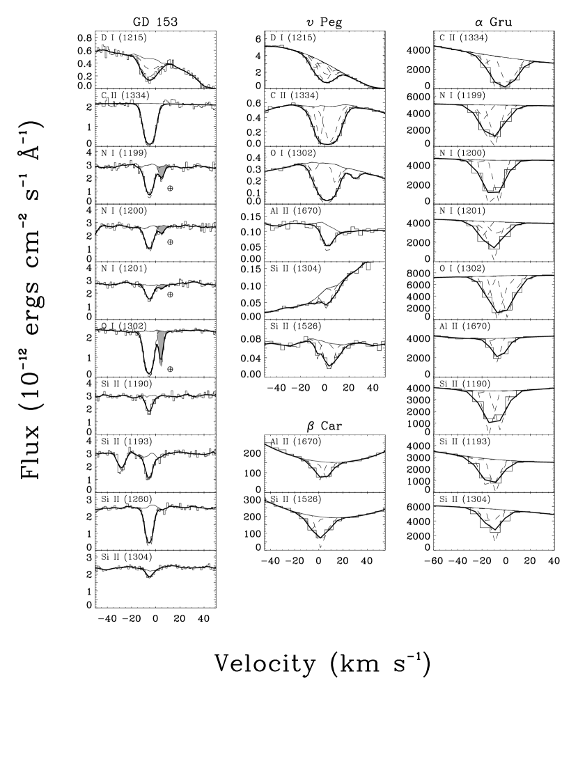
Figure 5: Continuation of Figure 1. The shaded absorption component are due to terrestrial airglow.

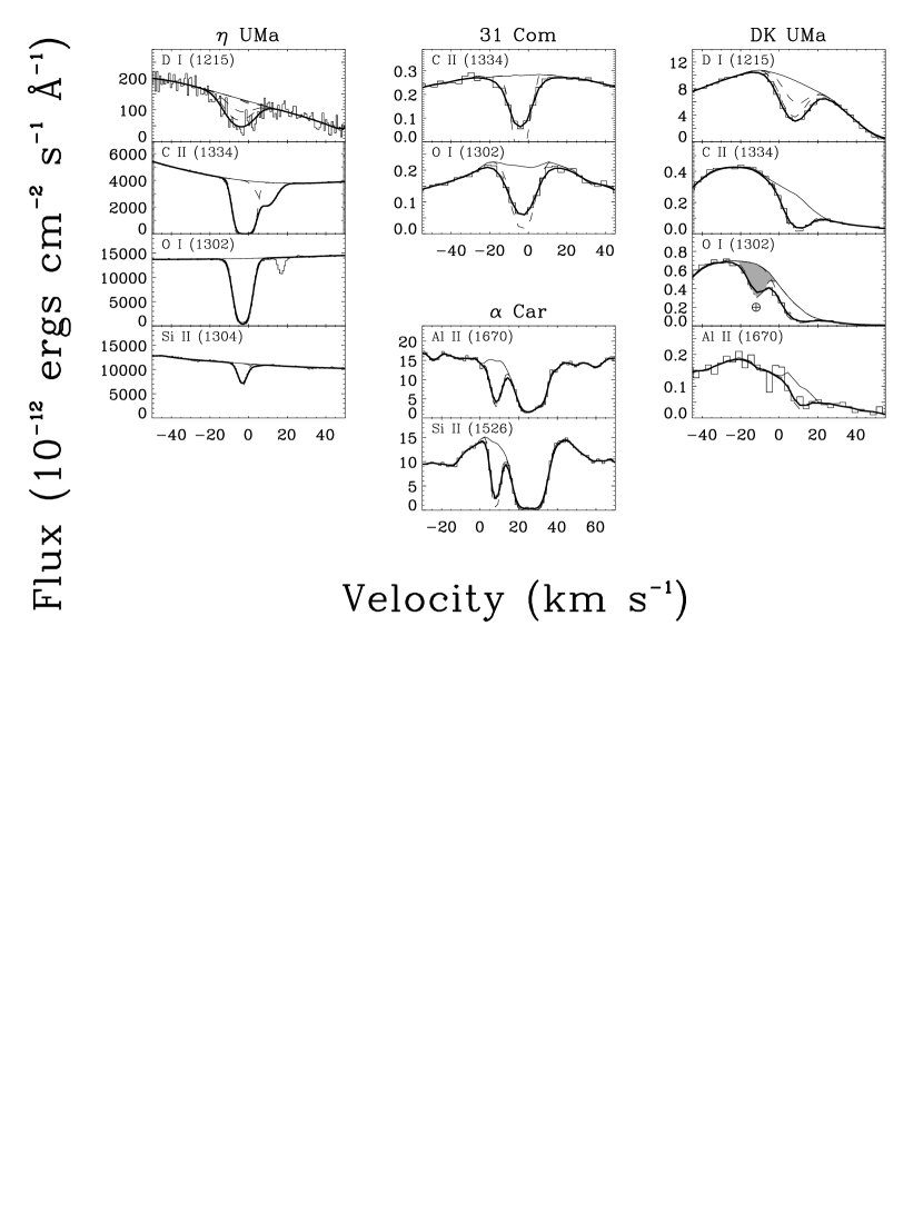
Figure 6: Continuation of Figure 1. The shaded absorption component is due to terrestrial airglow.

Figures 1-6 show our fits to the LISM absorption lines that were observed in the 1200-1800 Å spectral range and have not yet been published (see Table 2 for a list of the observational parameters). All of the spectra are shown with a heliocentric velocity scale, together with our estimate of the stellar continuum (thin solid lines), the best fits to the absorption by each interstellar component (dashed lines), and the total interstellar absorption convolved with the instrumental profile (thick solid lines). Table 3 presents an inventory of detected LISM absorption toward all 41 stars within 100 pc that have both a high resolution heavy ion detection and at least one moderate to high resolution detection of a light ion. We differentiate the new measurements presented in this work, with those already analyzed in the literature. Of the 41 sightlines listed in Table 3, 33 have new LISM absorption line observations.

The LISM absorption lines are fit using standard techniques (Linsky & Wood, 1996; Piskunov et al., 1997; Dring et al., 1997; Redfield & Linsky, 2002). This involves estimating the stellar continuum, determining the fewest number of absorption components required to obtain a satisfactory fit, convolving the absorption feature with an instrumental line spread function, and fitting all lines of the same ion simultaneously. Determining the stellar continuum is usually straightforward when dealing with high resolution data, and systematic errors in this procedure are further reduced when several resonance lines of the same ion are fit simultaneously. Because the central wavelength of the interstellar absorption is different for each line of sight, the placement of the unobserved stellar flux for some cases can be both difficult and the dominant source of error. In most cases, the “continuum” against which the absorption is measured can be determined by fitting a simple polynomial to spectral regions just blueward and redward of the interstellar absorption. Of the 206 interstellar absorption spectra shown in Figures 1-6 (as well as those shown in Appendix A), 68% of the continua were determined in this straightforward way.

Occasionally, a simple polynomial is not sufficient to accurately estimate the missing stellar continuum. We employ three additional techniques to accurately estimate the continuum: mirroring, similarity, and simultaneous fitting. The mirroring technique for estimating the unobserved stellar flux involves reflecting the emission line about the stellar photospheric radial velocity. If the interstellar absorption is far from line center, typically because of the high radial velocity of the star, this technique can be very useful in estimating the stellar flux. Since these circumstances are not very common, we used this method for estimating the continuum for only 5% of the sample. Fitting the C II line of 36 Oph A and 70 Oph (see Figure 1) are examples of this technique.

A stellar emission line with LISM absorption is often a member of a multiplet. Because the other members of the multiplet are not resonance transitions, no LISM absorption is seen against these emission lines. The shape of this line can be used to help reconstruct the continuum of the absorbed resonance line. This is particularly useful with lines that may or may not exhibit self-reversals at line center or multiple Gaussian profiles, such as Mg II, C II, and O I, as well as lines that are severely blended with additional lines or a rising stellar continuum, such as Fe II. Although the line width and integrated flux vary among multiplet members, the shapes of the line profiles are often very similar. Examples of this technique are the C II lines of $\epsilon$ Eri (see Figure 1), and the O I lines of $\beta$ Gem, $\beta$ Cet, and $\iota$ Cap (see Figures 2, 3, and 5, respectively). This method is used for estimating 13% of the continua in this sample.

One of the strengths of this sample, is that there are often several absorption lines for the same ion, particularly N I, Si II, Mg II, and Fe II. Because the oscillator strengths are known, the measured absorption in one line, predicts the absorption for all of the other resonance lines of the same ion. In this way, we can estimate continua for low signal-to-noise (S/N) absorption features in moderate resolution data for an ion, as long as we have at least one other reasonably simple absorption feature of the same ion. By simultaneously fitting all of the absorption features of the same ion, we can make a reasonable estimate of the continuum that is consistent with each absorption line. Although this technique can cause some curious continua estimates, it is the best method for reducing the systematic errors involved in continua placement. In only a few cases, approximately 14%, does this method produce results that deviate from a simple polynomial continuum estimation. Some examples include the Si II lines of GD 153 (see Figure 5) and the Fe II lines of HD 184499.

Once the continuum has been determined, we apply the minimum number of absorption components for a satisfactory fit to the spectra. Adding more absorption components invariably improves the goodness-of-fit metric ($\chi^{2}$). We use the F-test to determine whether the improvement in the fit is statistically significant (Bevington & Robinson, 1992), and allows us to determine the minimum number of necessary absorption components in an objective way.

The instrumental line spread functions assumed in our fits for GHRS spectra are taken from Gilliland (1994) and for STIS spectra from Sahu et al. (1999). The rest wavelengths and oscillator strengths of the lines used in our fits are taken from Morton (1991) with updates from D.C. Morton (2003, private communication). We fit all lines of each ion simultaneously in order to obtain the most robust parameters for the interstellar absorption. The difference in oscillator strengths between the various lines can be very useful in constraining the interstellar parameters, the stellar continuum level, and the number of absorption components. By providing an independent measure of the same absorbing column using absorption lines with different optical depths and at different locations relative to the stellar continuum, our analysis of several lines of the same ion reduces the effect of systematic errors, in particular from saturation and line blends, that result from the measurement of only one line.

Occasionally, absorption features due to terrestrial material are detected in spectra of O I and N I (see HZ 43, GD 153, and DK UMa, in Figures 4-6). The absorption is easily identified because it is centered at the mean velocity of the Earth during the time of observation, and because it is often also seen in the other members of the multiplet, where no LISM absorption is detected. The airglow absorption features are easily modeled and do not adversely affect the fit to the LISM absorption lines.

For each absorption component there are three fit parameters: the central velocity ($v$ [km s^-1]), the Doppler width ($b$ [km s^-1]), and the column density ($N_{\rm ion}$ [cm^-2]). The central velocity corresponds to the mean projected velocity of the absorbing material along the line of sight to the star. If, as a first approximation, we assume that the warm partially ionized material in the solar neighborhood exists in small, homogeneous cloudlets each moving with a single bulk velocity, then each absorption component will correspond to a single cloudlet, and its velocity is the projection of its three-dimensional velocity vector along the line of sight. The Doppler width parameter is related to the temperature ($T$ [K]) and nonthermal velocity ($\xi$ [km s^-1]) of the interstellar material by the following equation:

$$b^{2}=\frac{2kT}{m}+\xi^{2}=0.016629\left(\frac{T}{A}\right)+\xi^{2},$$ (1)

where $k$ is Boltzmann’s constant, $m$ is the mass of the ion observed, and $A$ is the atomic weight of the element in atomic mass units (where $A$ can range from $A_{\rm D}=2.01410$ to $A_{\rm Fe}=55.847$). The Doppler width parameter, or line width, of an ion with a large atomic weight is more sensitive to turbulent broadening than thermal broadening. The column density measures the amount of material along the line of sight to the star. If we assume homogeneous cloudlets with constant density, then the column density will be directly proportional to the cloud thickness. The compilation of all measurements for stars within 100 pc provides an important database for the analysis of the structure of the LISM. The velocity structure is discussed in Section 3.1, the Doppler width parameter structure is discussed in Section 3.2, and the column density structure is discussed in Section 3.3.

In order to extract as much information as possible from the UV observations of LISM absorption lines, we apply knowledge of the velocity structure along the line of sight derived from high resolution spectra of intrinsically narrow absorption lines of Fe II and Mg II to the fitting of the moderate resolution spectra of the lower mass, and thus, intrinsically broader absorption lines. For example, an Fe II absorption line formed by interstellar material at the canonical LISM temperature, $\sim\,7000$ K, and with no turbulent broadening will have a Doppler line width of $b\,=\,1.44$ km s^-1, whereas the D I absorption line for the same conditions will have $b\,=\,7.60$ km s^-1. To fully resolve the interstellar Fe II absorption feature requires a spectral resolution of $R\,=\,\lambda/\Delta\lambda\,>\,$200,000, whereas the D I feature requires a resolution of $R\,>\,$40,000. If the heavy ions accurately trace the same collection of gas as the light ions, then the required resolving power can decrease, as the atomic weight of the ion decreases, provided that the kinematic structure along the line of sight has already been determined from the analysis of intrinsically narrow lines observed at high resolution.

In this paper, we take advantage of such high resolution observations of Fe II and Mg II lines presented by Redfield & Linsky (2002) to fit moderate resolution data of the same sightlines. In particular, we fit the same number of velocity components to the light ion spectra that were necessary in the high resolution spectra. In practice, the vast majority of light ion absorption spectra have enough spectral resolution and signal-to-noise to independently constrain the number of components and their central velocities. However, in cases where the absorption components are severely blended, or the S/N is particularly poor, we use information from the high resolution fits to Fe II and Mg II. In only two sightlines, 70 Oph (C II, O I, and Si II) and HD 28568 (C II), the absorption features are so blended that we use the velocity information directly from the Mg II data to fit these spectra. In a handful of additional cases, the absolute velocity structure is not constrained, only the differences in central velocities are taken from the high resolution fits to constrain the light ion spectra.

Tables The Structure of the Local Interstellar Medium. II. Observations of D I, C II, N I, O I, Al II, and Si II toward Stars within 100 parsecs through The Structure of the Local Interstellar Medium. II. Observations of D I, C II, N I, O I, Al II, and Si II toward Stars within 100 parsecs list the interstellar absorption parameters and $1\sigma$ errors for all targets in Table 1 that show interstellar absorption in D I, C II, N I, O I, Al II, and Si II, respectively. The data in Tables The Structure of the Local Interstellar Medium. II. Observations of D I, C II, N I, O I, Al II, and Si II toward Stars within 100 parsecs-The Structure of the Local Interstellar Medium. II. Observations of D I, C II, N I, O I, Al II, and Si II toward Stars within 100 parsecs include our fits to the lines of sight shown in Figures 1-6. All errors quoted in the text, tables, and figures are $1\sigma$ error bars. In Table The Structure of the Local Interstellar Medium. II. Observations of D I, C II, N I, O I, Al II, and Si II toward Stars within 100 parsecs we list 1$\sigma$ errors in $\log N_{\rm DI}$ that for the best cases are as small as 0.01. For those lines of sight with only one velocity component and high S/N spectra, we can reliably interpolate the H I line profile in the neighborhood of the D I line to achieve this precision. Observations with moderate S/N, and/or several velocity components detected along the line of sight, typically have uncertainties in $\log N_{\rm DI}$ on the order of 0.1.

3 Discussion

The following discussion will be primarily a statistical analysis of the LISM absorption fit parameters discussed above. In future papers we will present more detailed analyses of the database, including the morphology, kinematics, and physical properties of identifiable structures (i.e. clouds) in the LISM. The location of all stars listed in Table 1 are shown in Galactic coordinates in Figure 7. Although spatial coverage overall is fairly good, there are areas of the sky that are poorly sampled, while others are densely sampled.

3.1 Velocity Distribution

Because the focus of this paper is the fitting of relatively broad absorption lines of low mass ions with moderate resolution data, the measurement of velocity centroids is unlikely to improve the accuracy obtained from fits to the high resolution spectra of narrow absorption lines. However, our analysis of the low mass ion profiles provides an opportunity to measure the consistency of the observed velocity centroids for a particular absorber. By comparing the measured absorption velocities of many resonance lines along the same sightline, we can test: (1) the implicit assumption that all of the observed ions sample the same collection of gas, and will therefore have the same observed projected velocity, and (2) the magnitude of systematic errors involved in comparing observations obtained with different spectral resolutions and observed with different instruments (e.g. GHRS or STIS). Ionization models of the LISM by Slavin & Frisch (2002) indicate that all of the measured ions discussed in this paper are expected to be the dominate ion of the element, and therefore we expect them all to sample the same collection of gas.

Each individual sightline now includes multiple measurements with different ions of the projected velocity of each interstellar absorber (cloud) along the line of sight. Figure 8 shows the distribution of the standard deviation about the weighted mean of these velocity measurements for each particular absorber. If all ions sample the same collection of gas and all of our instruments were infinitely precise and perfectly calibrated, then the standard deviation should be $\sim\,0$. Although there is a distribution of standard deviations, it is strongly peaked at 0. Therefore, all of the measured ions for each cloud appear to sample the same collection of gas. The dashed line indicates a Gaussian fit to the distribution, which well characterizes the data. The Gaussian has a standard deviation of $\sigma_{\rm G}\,=\,0.59\,$km s^-1. We believe that this is a good estimate of the typical systematic error involved in measuring LISM absorption lines in moderate and high resolution spectra observed with the GHRS and STIS instruments. Because we are comparing a large number of individual observations, each with its own systematic errors particular to each absorption feature (i.e. continuum placement, degree of blending with other lines, etc…), the distribution of systematic errors approaches a random distribution. Therefore, the range of standard deviations for all of the central velocity measurements of a particular absorber (cloud) should and does approximate a Gaussian distribution with a rather small half width.

3.2 Doppler Width Parameter Distribution

The observed value of the Doppler width parameter ($b$) is a measure of the temperature ($T$) and turbulent velocity ($\xi$). The relationship is provided by Equation 1. With increasing atomic mass, the Doppler width parameter is influenced less by thermal broadening and more by turbulence or unresolved clouds along the line of sight. In Figure 9, the Doppler width parameter distribution is plotted for all ions, from the heaviest ion, Fe II, at the top, to the lightest ion, D I, at the bottom. The increase in line width for ions with decreasing atomic weight demonstrates that thermal broadening becomes increasingly important relative to turbulent broadening for the lightest ions. The Doppler width parameter distributions of the heaviest ions look very similar, probably because turbulent broadening completely dominates over the thermal broadening, thereby making the Doppler width parameter independent of atomic mass. The weighted mean and standard deviation of the Doppler width parameter for all of the ions is given in Table 10. The high Doppler width parameter tails for all of the distributions likely results from unresolved blends (Welty, Morton, & Hobbs, 1996). We attempt to minimize the occurrence of unresolved blends by, (1) observing many absorbing ions along the same line of sight, (2) observing optically thin absorption lines where individual cloud absorbers are more easily identified, (3) using high resolution observations, and (4) observing the shortest ($\leq\,$100 pc) lines of sight to keep the absorption profile relatively simple. However, despite our efforts, we may not be resolving all the absorbers. Observations with higher spectral resolution would help to disentangle the component structure and to fully resolve the smallest line widths, allowing us to investigate more accurately the thermal and nonthermal characteristics of warm clouds in the LISM.

Comparing the line widths of various atomic species with a range of atomic masses, is a powerful technique for measuring the temperature and turbulent velocity of clouds in the LISM. In Figure 10, we plot the mean Doppler width parameters, inversely weighted by the variance of each measurement, of the entire dataset, as a function of atomic weight. We fit the weighted mean values to Equation 1 to calculate a typical temperature and turbulent velocity for the LISM in the aggregate. The variations in temperature and turbulent velocity among the various warm clouds in the LISM will be discussed in detail in Redfield & Linsky (2003). As a whole, the LISM can be roughly characterized by a temperature of $6900^{+2400}_{-2100}\,$K and a turbulent velocity of $1.67^{+0.57}_{-0.71}$ km s^-1, where the error bars likely reflect the intrinsic range in these parameters rather than measurement uncertainties (Redfield & Linsky, 2003).

3.3 Column Density Distribution

The observed column densities give the number of ions along the line of sight to the background source. If we assume a homogeneous medium with constant gas density, the column density is directly proportional to the distance that the line of sight traverses through the cloud. If the gas density is known, the column density of an individual absorption component is a direct measurement of the cloud thickness, which is vital to understanding the morphology of the LISM. The measured abundances also provide information on the degree of ionization and depletion of ions in the LISM. These characteristics can vary from cloud to cloud and even within a single cloud structure.

The cloud column density distribution function for each ion is given in Figure 11. The distribution functions vary due to differences in cosmic abundances, depletion patterns, and ionization structure. The weighted mean and standard deviation of the individual cloud column density for all of the ions are given in Table 10. The relatively small dispersion in the column densities, particularly in D I, suggests that nearby clouds in the LISM may have similar sizes. If we assume a constant D/H ratio of $1.5\,\times\,10^{-5}$ in the LISM (Linsky, 1998; Moos et al., 2002), and a constant H I number density of 0.1 cm^-3 (Redfield & Linsky, 2000), then we can use the weighted mean and standard deviation of the D I column density distribution to estimate a typical length scale for clouds in the LISM. This calculation results in a mean length of $2.2^{+1.7}_{-1.0}$ pc, and a range from 0.1 pc to 11 pc.

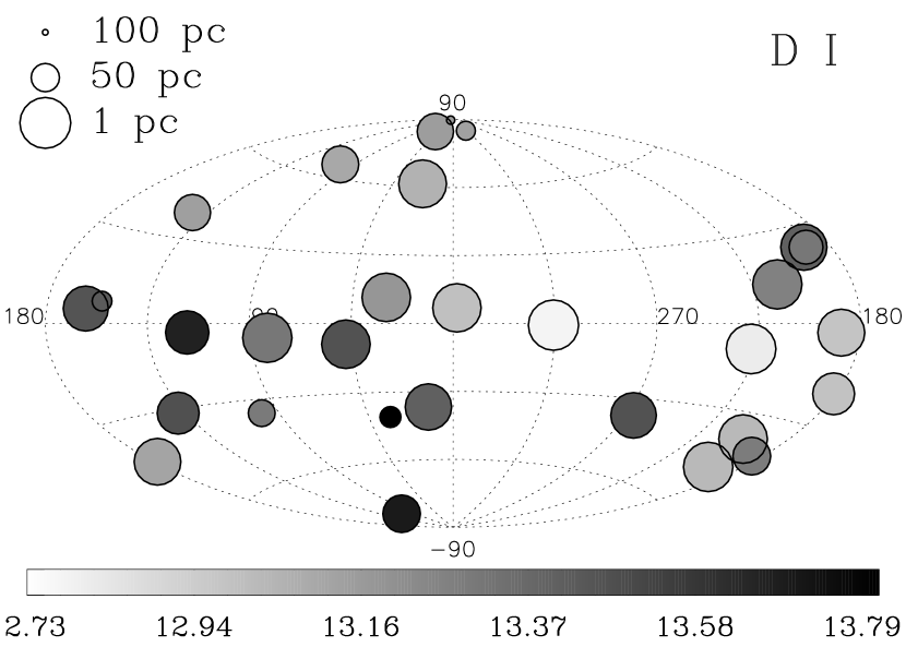
Figure 12: The total column density of D I along different lines of sight is shown in Galactic coordinates. The size of each symbol is inversely proportional to the distance to the star, and the shading of the symbol indicates the total column density, as shown by the scale at the bottom of each plot. Tables 1, 3, and The Structure of the Local Interstellar Medium. II. Observations of D I, C II, N I, O I, Al II, and Si II toward Stars within 100 parsecs can be used to identify each particular sightline. The total column densities are clearly spatially correlated. The highest column densities tend to be in the southern Galactic Center direction, and the lowest column densities tend to be in the northern anti-Galactic Center direction.

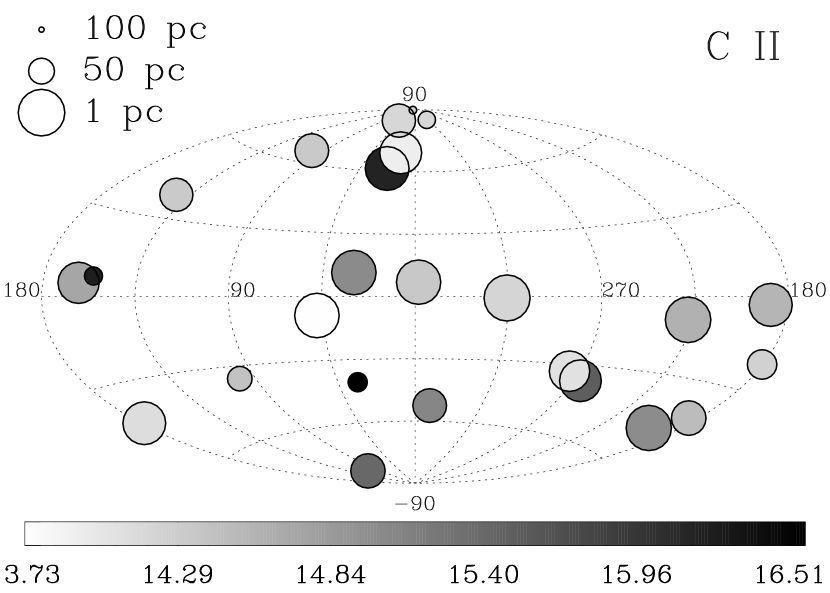
Figure 13: Similar to Figure 12, but displaying the total column density of C II in Galactic coordinates. Tables 1, 3, and The Structure of the Local Interstellar Medium. II. Observations of D I, C II, N I, O I, Al II, and Si II toward Stars within 100 parsecs can be used to identify each particular sightline.

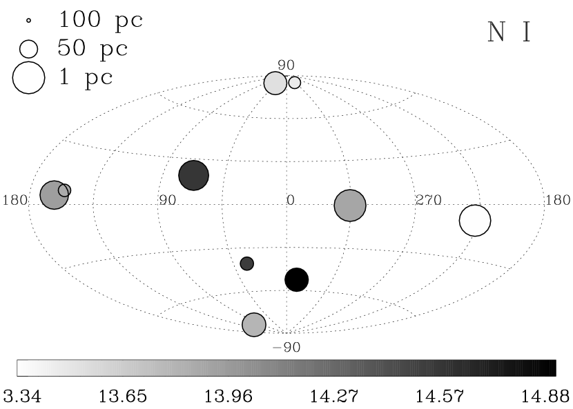
Figure 14: Similar to Figure 12, but displaying the total column density of N I in Galactic coordinates. Tables 1, 3, and The Structure of the Local Interstellar Medium. II. Observations of D I, C II, N I, O I, Al II, and Si II toward Stars within 100 parsecs can be used to identify each particular sightline.

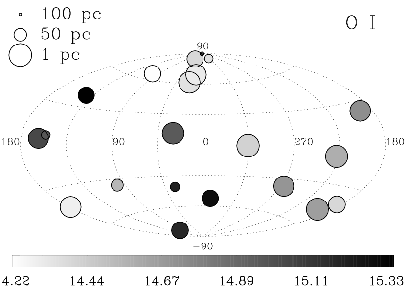
Figure 15: Similar to Figure 12, but displaying the total column density of O I in Galactic coordinates. Tables 1, 3, and The Structure of the Local Interstellar Medium. II. Observations of D I, C II, N I, O I, Al II, and Si II toward Stars within 100 parsecs can be used to identify each particular sightline.

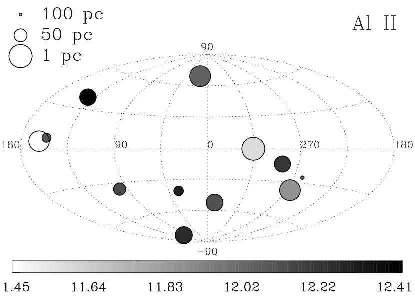
Figure 16: Similar to Figure 12, but displaying the total column density of Al II in Galactic coordinates. Tables 1, 3, and The Structure of the Local Interstellar Medium. II. Observations of D I, C II, N I, O I, Al II, and Si II toward Stars within 100 parsecs can be used to identify each particular sightline.

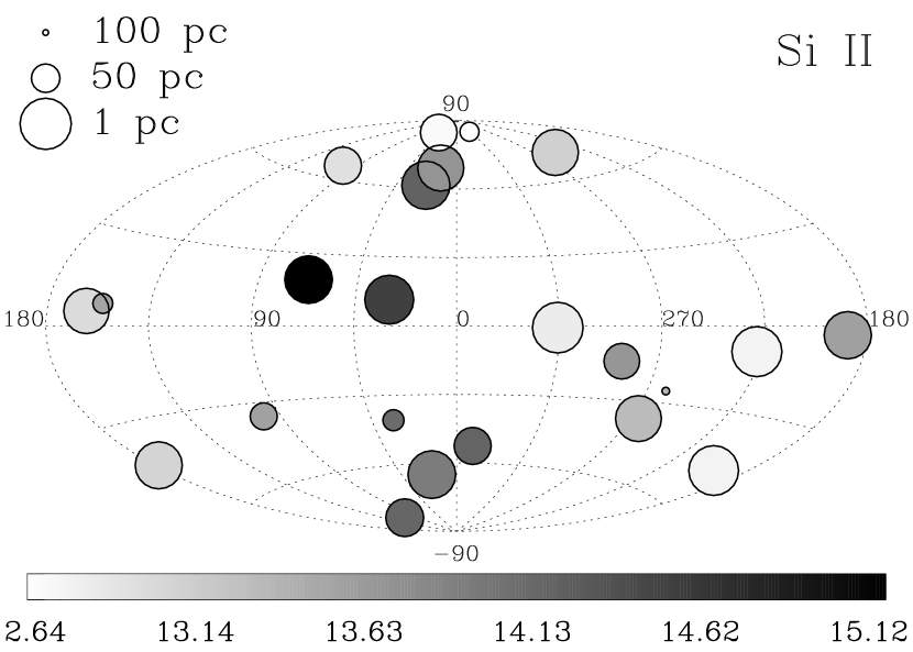
Figure 17: Similar to Figure 12, but displaying the total column density of Si II in Galactic coordinates. Tables 1, 3, and The Structure of the Local Interstellar Medium. II. Observations of D I, C II, N I, O I, Al II, and Si II toward Stars within 100 parsecs can be used to identify each particular sightline.

In Figures 12-17, the total column density for each ion is shown in Galactic coordinates. The size of a symbol is inversely proportional to the target’s distance, and the shading of a symbol indicates the total column density, as shown by the scale at the bottom of each plot. The total column densities are clearly spatially correlated. As was found by Génova et al. (1990), the highest column densities tend to be for lines of sight south of the Galactic Center, and the lowest column densities tend to be in the northern anti-Galactic Center direction. However, exceptions to this generalization exist. Good spatial coverage of the sky and of objects at various distances is crucial to understanding the morphology of the LISM.

4 Conclusions

We present a compilation of LISM absorption line measurements of ions in the spectral range from 1200-1800 Å, which includes lines of D I, C II, N I, O I, Al II, and Si II. This work is a companion paper to the research presented by Redfield & Linsky (2002) on the high resolution LISM absorption lines of the heavy ions Fe II, Ca II and Mg II. These two papers provide a complete inventory of available LISM measurements in the UV that can be used to determine the physical properties of the LISM and to test models of the structure of the gas in our local environment. The results of this work can be summarized as follows:

1. We take advantage of the known kinematic structure along a line of sight, obtained from high resolution observations of intrinsically narrow (high resolution) absorption lines (Redfield & Linsky, 2002), to accurately measure the LISM absorption features of intrinsically broad (low mass ion) lines. We successfully fit the absorption lines with this technique, even with moderate resolution spectra. This greatly enlarges the number of sightlines with useful LISM absorption line measurements.

2. The central velocity of a particular absorbing cloud is now measured using many resonance lines of different ions. The central velocity measurement for a given velocity component made with two different instruments (GHRS and STIS) and with a range of spectral resolutions have a standard deviation of only 0.59 km s^-1.

3. The distribution of Doppler widths shows a systematic increase as the atomic weight of the absorbing ion decreases. This demonstrates that thermal broadening becomes more important compared to turbulent broadening with decreasing ion mass. For the LISM in aggregate, we measure a temperature of $6900^{+2400}_{-2100}\,$K and a turbulent velocity of $1.67^{+0.57}_{-0.71}$ km s^-1. Variations in temperature and turbulent velocity are significant in the LISM as is discussed in detail in Redfield & Linsky (2003).

Appendix A High Resolution Observations of Fe II and Mg II

A survey of all available high resolution observations of Fe II and Mg II absorption along sightlines within 100 pc was presented by Redfield & Linsky (2002). We have expanded the survey in this work to include other ions, such as, D I, C II, N I, O I, Al II, and Si II. For three lines of sight with new light ion measurements presented here, we also have new heavy ion observations that we analyzed before fitting the moderate to high resolution light ion spectra. We include in this appendix the new high resolution Fe II line (2600.1729 Å, 2586.6500 Å, 2382.7652 Å, 2374.4612 Å, 2344.2139 Å) and Mg II h and k line (2803.5305 Å and 2796.5318 Å) observations toward stars within 100 pc, since the publication of Redfield & Linsky (2002). These sightlines are listed in Table 11, while the particular observational details are given in Table 12.

Figures 18-20 show our best fits to the new Mg II and Fe II observations. Tables The Structure of the Local Interstellar Medium. II. Observations of D I, C II, N I, O I, Al II, and Si II toward Stars within 100 parsecs and The Structure of the Local Interstellar Medium. II. Observations of D I, C II, N I, O I, Al II, and Si II toward Stars within 100 parsecs give the absorption line fit parameters for Mg II and Fe II, respectively, for all targets shown in Figures 18-20. In addition, some errors in the tables of Redfield & Linsky (2002) are corrected here. Tables The Structure of the Local Interstellar Medium. II. Observations of D I, C II, N I, O I, Al II, and Si II toward Stars within 100 parsecs and The Structure of the Local Interstellar Medium. II. Observations of D I, C II, N I, O I, Al II, and Si II toward Stars within 100 parsecs are meant to be continuations of Tables 3 and 4 in Redfield & Linsky (2002).

Based on the number of observed LISM absorbers for each ion, given in Table 10, the best sampling of the distribution of LISM clouds will come from Mg II and Fe II. By comparing the number of velocity components (clouds) along a given sightline with the distance of the background star, we can investigate the rough distribution of warm clouds within 100 pc. In Figure 21, the average number of clouds along the line of sight toward stars located in 10 pc bins is compared for the heavy ions, Fe II, Ca II, and Mg II, based on the analysis of only high-resolution spectra presented here and in Redfield & Linsky (2002). It is remarkable that the average number of clouds remains nearly constant out to 100 pc. Only a very slight increasewith stellar distance is detected, indicating that the distribution of clouds in the LISM is not uniform, but instead is concentrated near the Sun. The specific morphology of the LISM can induce biases into these estimates, particularly if only one star is used in a particular distance bin, as is the case for Fe II and Mg II at distances $>\,70$ pc. These particular sightlines happen to be at high latitudes, where little LISM material is detected (see Figures 12 to 17). The specific morphology of the LISM will be the subject of a future paper in this series.

Previous estimates of the number density of clouds in the ISM have been between 8 and 10 cloud components per kpc (Spitzer, 1978). These, relatively low resolution observations, were of more distant sightlines that traversed a more varied ISM environment and more clouds. Our estimate, as shown in Figure 21 is $\sim\,20$ clouds per kpc. Although we only sample a relatively simple ISM environment, namely warm partially ionized clouds within the Local Bubble, our data are not severely blended because of the short lines of sight and high spectral resolution. The cloud density estimated from more distant sightlines may suffer from such severe blending that many clouds are undetected, leading to an underestimate of the number of clouds along the line of sight.

Figure 1: Fits to the light ion LISM absorption lines for 32 lines of sight toward stars located within 100 pc. The name of the target star is given above each group of plots, and the resonance line ion (D I, C II, N I, O I, Al II, or Si II) and wavelength (Å) are identified within each individual plot. The data are shown in histogram form. The thin solid lines are our estimates of the intrinsic stellar flux across the absorption lines. The dashed lines are the best-fit individual absorption lines before convolution with the instrumental profile. The thick solid line represents the combined absorption fit after convolution with the instrumental profile. The spectra are plotted versus heliocentric velocity. The parameters for these fits are given in Tables The Structure of the Local Interstellar Medium. II. Observations of D I, C II, N I, O I, Al II, and Si II toward Stars within 100 parsecs through The Structure of the Local Interstellar Medium. II. Observations of D I, C II, N I, O I, Al II, and Si II toward Stars within 100 parsecs.

Figure 2: Continuation of Figure 1.

Figure 3: Continuation of Figure 1.

Figure 4: Continuation of Figure 1. The shaded absorption component are due to terrestrial airglow.

Figure 7: The location of all stars listed in Table 1 are shown in Galactic coordinates. All HST targets with high resolution spectra of Mg II and/or Fe II are indicated by the “$\times$” symbol. There are 80 sightlines within 100 pc, which currently have these heavy ion detections (see Redfield & Linsky (2002) and Appendix A of this work). Those stars that in addition, have moderate or high resolution spectra of any light ions, such as D I, C II, N I, and O I, are plotted as open circles. Of the 41 sightlines that have both high resolution observations of a heavy ion and at last one observation of a light ion at moderate or high resolution, new data are presented in this work for 33 lines of sight.

Figure 8: The distribution of standard deviations (the square root of the weighted average variance) about the weighted mean velocity centroid measurements in resonance lines of different ions for individual LISM components along the same line of sight. There are 87 individual components along 45 sightlines, where two or more resonance lines trace absorption from the same collection of local gas. The sightlines include those presented in this paper with both heavy and light ion observations, plus a few lines of sight with both Fe II and Mg II, but no light ion observations, as discussed by Redfield & Linsky (2002) and in Appendix A. Each absorption line provides an independent measurement of the projected velocity of the absorbing gas. However, due to random and systematic errors, those measurements are distributed about the true value. This figure shows the standard deviation about the weighted mean for all of the velocity centroid measurements for each component along each line of sight. The dashed line indicates a Gaussian distribution with a mean of 0 km s^-1, and a standard deviation of 0.59 km s^-1. The large majority (78%) of velocity components agree to within 1.0 km s^-1. The outliers are most likely caused by unresolved blends, or large systematic errors in the instrumental wavelength calibration. The bin size used is 0.2 km s^-1.

Figure 9: The Doppler width parameter distribution for eight ions, from the heaviest ion, Fe II, at the top, to the lightest ion, D I, at the bottom. The bin size used is 0.25 km s^-1. The dashed lines indicate the weighted mean Doppler width. The weighted mean, standard deviation of the weighted mean, and the total number of observations (N) of each ion are presented in Table 10. A clear shift to larger line widths is seen toward lighter ions, indicating that for the heaviest ions turbulent broadening dominates and the Doppler width parameter is independent of atomic mass, while for the lightest ion thermal broadening dominates.

Figure 10: The weighted mean Doppler width parameter for all LISM absorbers, is plotted as a function of the atomic weight of the observed ion. The error bars indicate the weighted standard deviation of the sample. The ions are identified along the top axis. The best fit temperature and turbulent velocity for the LISM in aggregate is given in the plot, and the best fit curve is displayed by the solid line, as described by Equation 1. Variations in temperature and turbulent velocity do exist among the various warm clouds in the LISM, as discussed in detail in Redfield & Linsky (2003).

Figure 11: The column density distribution for individual clouds is given for each ion. The dashed lines indicate the weighted mean column densities. The weighted mean, standard deviation of the weighted mean, and the total number of observations (N) of each ion are presented in Table 10. The variations among the various ions results from different cosmic abundances, depletions, and ionization structure.

Figure 18: Fits to the Mg II and Fe II lines for 16 lines of sight toward stars within 100 pc. These sightlines complement the Mg II and Fe II LISM absorption line sample presented by Redfield & Linsky (2002). The name of the target star is given above each group of plots, and the resonance line is identified within each individual plot. The data are shown in histogram form. The thin solid lines are our estimates for the intrinsic stellar flux across the absorption lines. The dashed lines are the best-fit individual absorption lines before convolution with the instrumental profile. The thick solid line represents the combined absorption fit after convolution with the instrumental profile. The spectra are plotted versus heliocentric velocity. The parameters for these fits are given in Table The Structure of the Local Interstellar Medium. II. Observations of D I, C II, N I, O I, Al II, and Si II toward Stars within 100 parsecs for Mg II and in Table The Structure of the Local Interstellar Medium. II. Observations of D I, C II, N I, O I, Al II, and Si II toward Stars within 100 parsecs for Fe II.

Figure 19: Continuation of Figure 18.

Figure 20: Continuation of Figure 18.

Figure 21: The distribution of the average number of velocity components (clouds) along sightlines as a function of the distance to the background star. The binsize is 10 pc. The total number of sightlines included in the average is given near the bottom of each bin. Although the distance to each cloud is not known, the distance to the star provides an upper limit. The specific morphology of the LISM can induce biases into the distribution. For example, the sharp decline in the average number of absorbers for Fe II and Mg II at distances approaching 100 pc, results from the few stars observed at these distances being located at high latitudes, where little LISM material is detected (see Figures 12 to 17). The relatively constant average number of absorbers with distance indicates that the distribution of LISM clouds within the Local Bubble is not uniform but instead is concentrated close to the Sun.

Table 1: Parameters for Stars within 100 pc with Light Ion Observations

HD	Other	Spectral	$m_{\rm V}$	$v_{\rm R}$	$l$	$b$	distance	$v_{\rm{LIC}}$	$v_{\rm{G}}$
#	Name	Type		(km s-1)	(∘)	(∘)	(pc)	(km s-1)	(km s-1)
128620	$\alpha$ Cen A	G2V	–0.0–	–24.6	315.7	0–0.7	01.3	–15.6	–18.0
128621	$\alpha$ Cen B	K1V	1.3	–20.7	315.7	0–0.7	01.3	–15.6	–18.0
48915	$\alpha$ CMa A	A1V	–1.5–	0–7.6	227.2	0–8.9	02.6	–19.5	–21.6
48915B	$\alpha$ CMa B	DA	8.4	$\cdots$	227.2	0–8.9	02.6	–19.5	–21.6
22049	$\epsilon$ Eri	K2V	3.7	–15.5	195.8	–48.1	03.2	–21.6	–25.7
201091	61 Cyg A	K5V	5.2	–64.3	082.3	0–5.8	03.5	0–5.1	0–4.7
61421	$\alpha$ CMi	F5V	0.3	0–3.2	213.7	–13.0	03.5	–19.7	–21.1
26965	40 Eri A	K1V	4.4	–42.2	200.8	–38.1	05.0	–23.2	–27.2
165341	70 Oph	K0V	4.0	0–6.9	029.9	–11.4	05.1	–23.5	–26.4
187642	$\alpha$ Aql	A7V	0.8	–26.1	047.7	0–8.9	05.1	–17.1	–18.2
155886	36 Oph A	K0V	5.3	0–0.6	358.3	–06.9	05.5	–25.2	–28.4
131156A	$\xi$ Boo A	G8V	4.7	–03.0	023.1	–61.4	06.7	–17.7	–21.5
216956	$\alpha$ PsA	A3V	1.2	–06.5	020.5	–64.9	07.7	0–3.6	0–1.9
172167	$\alpha$ Lyr	A0V	0.0	–13.9	067.5	–19.2	07.8	–13.5	–15.2
39587	$\chi^{1}$ Ori	G0V	4.4	–13.5	188.5	0–2.7	08.7	–24.9	–27.9
20630	$\kappa^{1}$ Cet	G5V	4.8	–19.9	178.2	–43.1	09.2	–22.8	–27.0
197481	AU Mic	M0	8.6	–01.2	012.7	–36.8	09.9	–15.3	–15.7
62509	$\beta$ Gem	K0III	1.2	–03.3	192.2	–23.4	10.3	–19.6	–21.0
102647	$\beta$ Leo	A3V	2.1	0–0.2	250.6	–70.8	11.1	0–3.4	0–6.1
124897	$\alpha$ Boo	K1.5III	–0.0–	0–5.2	015.1	–69.1	11.3	–15.5	–19.3
33262	$\zeta$ Dor	F7V	4.7	0–2.0	266.0	–36.7	11.7	–07.8	–09.4
34029	$\alpha$ Aur	G5III	0.1	–30.2	162.6	–04.6	12.9	–22.0	–24.6
36705	AB Dor	K1III	6.9	–33.0	275.3	–33.1	14.9	–04.3	0–5.3
432	$\beta$ Cas	F2IV	2.3	–11.3	117.5	0–3.3	16.7	–09.4	–11.3
11443	$\alpha$ Tri	F6IV	3.4	–12.6	138.6	–31.4	19.7	–18.0	–21.7
29139	$\alpha$ Tau	K5III	0.9	–54.3	181.0	–20.3	20.0	–25.5	–29.4
22468	HR 1099	G9V	5.9	–23.0	184.9	–41.6	29.0	–23.3	–27.4
4128	$\beta$ Cet	K0III	2.0	–13.0	111.3	–80.7	29.4	–08.2	–11.4
120315	$\eta$ UMa	B3V	1.9	–10.9	100.7	–65.3	30.9	0–5.8	0–8.1
209952	$\alpha$ Gru	B7IV	1.7	–11.8	350.0	–52.5	31.1	0–8.7	0–8.1
$\cdots$	HZ 43	DAw	12.70	–62.0	054.1	–84.2	32.0	0–8.9	–12.0
82210	DK UMa	G4IV	4.6	–27.2	142.6	–38.9	32.4	–09.4	–09.5
80007	$\beta$ Car	A2IV	1.7	–5.0	286.0	–14.4	34.1	0–2.3	0–2.8
62044	$\sigma$ Gem	K1III	4.3	–45.8	191.2	–23.3	37.5	–19.7	–21.0
28568	SAO 93981	F5V	6.5	–40.9	180.5	–21.4	41.2	–25.5	–29.3
220657	$\upsilon$ Peg	F8IV	4.4	–11.1	098.6	–35.4	53.1	–05.1	–07.6
203387	$\iota$ Cap	G8III	4.3	–11.5	033.6	–40.8	66.1	–11.8	–11.5
$\cdots$	G191-B2B	DAw	11.60	–05.0	156.0	–07.1	68.8	–20.3	–22.7
$\cdots$	GD 153	DAw	13.4	$\cdots$	317.3	84.8	70.5	–8.7	–12.0
111812	31 Com	G0III	4.9	.–1.4	115.0	–89.6	94.2	0–7.2	–10.2
45348	$\alpha$ Car	F0II	–0.7	20.5	261.2	–25.3	95.9	8.8	10.1

Table 2: HST Observational Parameters

HD	Other	Instrument	Grating	Spectral	Resolution	Exposure	PI	Program	Date
#	Name			Range		Time	Name	ID
				(Å)	($\lambda/\Delta\lambda$)	(s)
128620	$\alpha$ Cen A	STIS	E140H	1140-1335	114000	4695.0	LINSKY	7263	1999 Feb 12
		STIS	E140H	1315-1517	114000	4695.0	LINSKY	7263	1999 Feb 12
		STIS	E140H	1497-1699	114000	4695.0	LINSKY	7263	1999 Feb 12
48915	$\alpha$ CMa A	GHRS	G160M	1645-1679	20000	1740.8	LALLEMENT	2461	1992 Aug 15
		GHRS	G160M	1651-1686	20000	108.8	WAHLGREN	3496	1993 Mar 16
		GHRS	G160M	1651-1686	20000	108.8	WAHLGREN	3496	1993 May 8
22049	$\epsilon$ Eri	STIS	E140M	1140-1735	45800	5798.0	JORDAN	7479	2000 Mar 17
165341	70 Oph	STIS	E140M	1140-1735	45800	7809.0	AYRES	8280	2000 Aug 23
187642	$\alpha$ Aql	GHRS	G160M	1315-1351	20000	544.0	WALTER	3950	1993 Apr 7
		GHRS	G160M	1317-1352	20000	435.2	SIMON	3737	1993 Apr 7
		GHRS	G140M	1201-1229	20000	761.6	SIMON	6083	1996 Mar 5
155886	36 Oph A	STIS	E140H	1170-1372	114000	8769.0	LINSKY	7262	1999 Oct 10
131156A	$\xi$ Boo A	STIS	E140M	1140-1735	45800	2450.0	TIMOTHY	7585	1998 Dec 16
216956	$\alpha$ PsA	GHRS	G160M	1524-1559	20000	3628.8	FERLET	2537	1993 Oct 31
		GHRS	G160M	1644-1679	20000	576.0	FERLET	2537	1993 Oct 31
172167	$\alpha$ Lyr	GHRS	G140M	1189-1217	20000	435.2	VIDAL-MADJAR	6828	1996 Aug 28
		GHRS	G160M	1185-1222	20000	435.2	VIDAL-MADJAR	6828	1996 Dec 23
39587	$\chi^{1}$ Ori	STIS	E140M	1140-1735	45800	6770.0	AYRES	8280	2000 Oct 3
20630	$\kappa^{1}$ Cet	STIS	E140M	1140-1735	45800	7805.0	AYRES	8280	2000 Sep 19
197481	AU Mic	STIS	E140M	1150-1735	45800	10105.0	LINSKY	7556	1998 Sep 6
62509	$\beta$ Gem	GHRS	ECH-A	1300-1307	100000	761.6	LINSKY	5647	1995 Sep 20
		GHRS	ECH-A	1300-1307	100000	761.6	LINSKY	5647	1995 Sep 20
102647	$\beta$ Leo	GHRS	G160M	1524-1559	20000	6912.0	FERLET	2537	1992 Jan 23
		GHRS	G160M	1645-1679	20000	1209.6	FERLET	2537	1992 Jan 24
124897	$\alpha$ Boo	STIS	E140M	1150-1735	45800	5208.0	AYRES	7733	1998 Aug 24
33262	$\zeta$ Dor	STIS	E140M	1140-1735	45800	6000.0	AYRES	8280	1999 May 1
34029	$\alpha$ Aur	STIS	E140M	1140-1735	45800	8113.0	DRAKE	8546	1999 Sep 12
36705	AB Dor	GHRS	G160M	1318-1354	20000	1305.6	WALTER	5181	1994 Nov 14-15
29139	$\alpha$ Tau	STIS	E140M	1140-1735	114000	10512.0	AYRES	9273	2002 Jan 3
22468	HR1099	STIS	E140M	1140-1735	45800	12225.0	AYRES	8280	1999 Sep 15
4128	$\beta$ Cet	STIS	E140M	1140-1735	100000	4737.0	LINSKY	8039	1999 Sep 13
120315	$\eta$ UMa	GHRS	ECH-A	1212-1218	100000	652.8	FRISCH	6886	1997 Jan 1
		GHRS	ECH-A	1298-1306	100000	217.6	FRISCH	6886	1997 Jan 1
		GHRS	ECH-A	1332-1339	100000	1171.4	FRISCH	6886	1997 Jan 1
209952	$\alpha$ Gru	GHRS	G160M	1174-1211	20000	460.8	SMITH	3941	1993 Jul 24
		GHRS	G160M	1277-1313	20000	230.4	SMITH	3941	1993 Jul 24
		GHRS	G160M	1309-1345	20000	230.4	SMITH	3941	1993 Jul 24
		GHRS	G160M	1642-1677	20000	230.4	SMITH	3941	1993 Jul 24
$\cdots$	HZ 43	STIS	E140H	1140-1335	114000	11656.0	SAHU	8595	2001 May 3
82210	DK UMa	STIS	E140M	1140-1735	45800	9300.0	AYRES	8280	2000 Feb 24
80007	$\beta$ Car	GHRS	G160M	1524-1559	20000	748.8	FERLET	2537	1993 Mar 16
		GHRS	G160M	1645-1679	20000	345.6	FERLET	2537	1993 Mar 16
28568	SAO 93981	STIS	E140M	1140-1735	45800	1065.0	BOHM-VITENSE	7389	1998 Nov 8
220657	$\upsilon$ Peg	STIS	E140M	1140-1735	45800	8226.0	AYRES	8280	2000 Jul 11
203387	$\iota$ Cap	STIS	E140M	1140-1735	45800	11651.0	AYRES	8280	2000 Apr 15
$\cdots$	G191-B2B	STIS	E140H	1140-1335	114000	2789.0	LEITHERER	8067	1998 Dec 17
		STIS	E140H	1497-1699	114000	2703.0	LEITHERER	8067	1998 Dec 17
		STIS	E140H	1140-1335	114000	8279.0	LEITHERER	8421	2000 Mar 16-17
		STIS	E140H	1497-1699	114000	8284.0	LEITHERER	8421	2000 Mar 17
		STIS	E140H	1140-1335	114000	1734.0	VALENTI	8915	2001 Sep 17
		STIS	E140H	1170-1372	114000	696.0	VALENTI	8915	2001 Sep 17
		STIS	E140H	1206-1408	114000	654.0	VALENTI	8915	2001 Sep 17
		STIS	E140H	1242-1444	114000	686.0	VALENTI	8915	2001 Sep 17
		STIS	E140H	1279-1481	114000	752.0	VALENTI	8915	2001 Sep 17
		STIS	E140H	1315-1517	114000	851.0	VALENTI	8915	2001 Sep 17
		STIS	E140H	1352-1554	114000	1038.0	VALENTI	8915	2001 Sep 17
		STIS	E140H	1388-1590	114000	1263.0	VALENTI	8915	2001 Sep 17
		STIS	E140H	1425-1627	114000	1636.0	VALENTI	8915	2001 Sep 17
		STIS	E140H	1461-1663	114000	1996.0	VALENTI	8915	2001 Sep 17
		STIS	E230H	1624-1896	114000	1314.0	VALENTI	8915	2001 Sep 18
$\cdots$	GD 153	STIS	E140H	1140-1335	114000	11697.0	SAHU	8595	2001 Mar 14
		STIS	E140H	1140-1335	114000	1851.0	SAHU	8595	2001 Mar 22
111812	31 Com	STIS	E140M	1140-1735	45800	7733.0	AYRES	8889	2001 Mar 13
45348	$\alpha$ Car	STIS	E140M	1140-1735	45800	2000.0	BROWN	7764	2002 Jun 11
		STIS	E140H	1497-1699	114000	1200.0	BROWN	7764	2002 Jun 11

Table 3: Inventory of LISM Absorption Line Detections

HD	Other	Moderate to High Resolution Light Ions						High Resolution Heavy Ions
#	Name	D I	C II	N I	O I	Al II	Si II	Mg II	Fe II
128620	$\alpha$ Cen A	($\surd$)	$\surd$	$\surd$	$\surd$	$\surd$	$\surd$	($\surd$)	($\surd$)
128621	$\alpha$ Cen B	($\surd$)						($\surd$)	($\surd$)
48915	$\alpha$ CMa A	($\surd$)	($\surd$)			$<$		($\surd$)	($\surd$)
48915B	$\alpha$ CMa B	($\surd$)	($\surd$)	($\surd$)	($\surd$)		($\surd$)	($\surd$)	($\surd$)
22049	$\epsilon$ Eri	($\surd$)	$\surd$		$\surd$	$<$	$\surd$	($\surd$)	($\surd$)
201091	61 Cyg A	($\surd$)						($\surd$)
61421	$\alpha$ CMi	($\surd$)						($\surd$)	($\surd$)
26965	40 Eri A	($\surd$)						($\surd$)
165341	70 Oph	$\surd$	$\surd$		$\surd$	$<$	$\surd$	($\surd$)	($\surd$)
187642	$\alpha$ Aql	$\surd$	$\surd$					($\surd$)	($\surd$)
155886	36 Oph A	($\surd$)	$\surd$					($\surd$)	($\surd$)
131156A	$\xi$ Boo A	$\surd$	$\surd$		$\surd$	$<$	$\surd$	($\surd$)
216956	$\alpha$ PsA					$<$	$\surd$		($\surd$)
172167	$\alpha$ Lyr			$\surd$			$\surd$		($\surd$)
39587	$\chi^{1}$ Ori	$\surd$	$\surd$			$<$	$\surd$	($\surd$)	($\surd$)
20630	$\kappa^{1}$ Cet	$\surd$	$\surd$		$\surd$	$<$	$\surd$	($\surd$)	($\surd$)
197481	AU Mic	$\surd$						($\surd$)
62509	$\beta$ Gem	($\surd$)			$\surd$			($\surd$)	($\surd$)
102647	$\beta$ Leo					$<$	$\surd$		($\surd$)
124897	$\alpha$ Boo		$\surd$		$\surd$	$\surd$	$\surd$	($\surd$)	($\surd$)
33262	$\zeta$ Dor	$\surd$	$\surd$		$\surd$	$\surd$	$\surd$	($\surd$)	($\surd$)
34029	$\alpha$ Aur	($\surd$)	($\surd$)	$\surd$	$\surd$	$\surd$	$\surd$	($\surd$)	($\surd$)
36705	AB Dor		$\surd$					($\surd$)
432	$\beta$ Cas	($\surd$)						($\surd$)	($\surd$)
11443	$\alpha$ Tri	($\surd$)						($\surd$)	($\surd$)
29139	$\alpha$ Tau	$\surd$						($\surd$)
22468	HR 1099	($\surd$)	$\surd$		$\surd$	$<$	$<$	($\surd$)
4128	$\beta$ Cet	($\surd$)	$\surd$	$\surd$	$\surd$	$\surd$	$\surd$	($\surd$)
120315	$\eta$ UMa	$\surd$	$\surd$		$\surd$		$\surd$	($\surd$)	($\surd$)
209952	$\alpha$ Gru		$\surd$	$\surd$	$\surd$	$\surd$	$\surd$	($\surd$)	($\surd$)
$\cdots$	HZ 43	$\surd$	$\surd$	$\surd$	$\surd$		$\surd$	($\surd$)	($\surd$)
82210	DK UMa	$\surd$	$\surd$	$<$	$\surd$	$\surd$	$<$	($\surd$)	($\surd$)
80007	$\beta$ Car					$\surd$	$\surd$		($\surd$)
62044	$\sigma$ Gem	($\surd$)						($\surd$)
28568	SAO 93981		$\surd$					($\surd$)
220657	$\upsilon$ Peg	$\surd$	$\surd$	$<$	$\surd$	$\surd$	$\surd$	($\surd$)	($\surd$)
203387	$\iota$ Cap	$\surd$	$\surd$	$\surd$	$\surd$	$\surd$	$\surd$	($\surd$)	($\surd$)
$\cdots$	G191-B2B	$\surd$	$\surd$	$\surd$	$\surd$	$\surd$	$\surd$	$\surd$	$\surd$
$\cdots$	GD 153	$\surd$	$\surd$	$\surd$	$\surd$		$\surd$		$\surd$
111812	31 Com	($\surd$)	$\surd$		$\surd$	$<$	$<$	($\surd$)	($\surd$)
45348	$\alpha$ Car					$\surd$	$\surd$	$\surd$	$\surd$

Note. — The $\surd$ symbol indicates a detection of LISM absorption. The $<$ symbol indicates no LISM absorption is detected, but an upper limit is provided. Symbols in parentheses indicate the LISM absorption analysis has already been presented in the literature. All detections that have not been previously analyzed are presented in this work. For the light ions, references for analyzed sightlines can be found in Tables The Structure of the Local Interstellar Medium. II. Observations of D I, C II, N I, O I, Al II, and Si II toward Stars within 100 parsecs-The Structure of the Local Interstellar Medium. II. Observations of D I, C II, N I, O I, Al II, and Si II toward Stars within 100 parsecs. Details regarding the heavy ion measurements can be found in Redfield & Linsky (2002) and Appendix A.

Table 4: Fit Parameters for D I ISM Velocity Components

HD	Other	Component	$v$	$b$	$\log N_{\rm DI}$	Reference
#	Name	#	(km s-1)	(km s-1)	$\log(\rm cm^{-2})$
128620	$\alpha$ Cen A	1	–18.2 $\pm$ 0.1	6.55 $\pm$ 0.27	12.799 $\pm$ 0.015	1
128621	$\alpha$ Cen B	1	–18.2 $\pm$ 0.1	6.88 $\pm$ 0.17	12.775 $\pm$ 0.009	1
48915	$\alpha$ CMa A	1	19.5	$\cdots$	12.43${}^{+0.14}_{-0.20}$	2
		2	13.7	$\cdots$	12.43${}^{+0.14}_{-0.20}$	2
48915B	$\alpha$ CMa B	1	17.6	8.14	12.81${}^{+0.09}_{-0.11}$	3
		2	11.7	5.66	$<$ 12.48	3
22049	$\epsilon$ Eri	1	20.5 $\pm$ 0.7	8.1 $\pm$ 0.4	13.03 $\pm$ 0.06	4
201091	61 Cyg A	1	–3.0	7.8	13.01	5
		2	–9.0	7.8	13.01	5
61421	$\alpha$ CMi	1	24.0 $\pm$ 0.10	7.59 $\pm$ 0.10	12.81 $\pm$ 0.03	6
		2	20.5 $\pm$ 0.10	7.59 $\pm$ 0.10	13.08 $\pm$ 0.04	6
26965	40 Eri A	1	21.4	8.2	13.03	5
165341	70 Oph	1	–26.2 $\pm$ 0.9	6.22 $\pm$ 0.54	12.95 $\pm$ 0.07	7
		2	–32.4 $\pm$ 0.9	4.95 $\pm$ 1.51	12.64 $\pm$ 0.24	7
		3	–42.9 $\pm$ 0.9	5.73 $\pm$ 1.40	12.27 $\pm$ 0.11	7
187642	$\alpha$ Aql	1	–18.4 $\pm$ 1.5	10.3 $\pm$ 1.0	13.09 $\pm$ 0.27	7 (see 8)
		2	–22.0 $\pm$ 1.5	10.3 $\pm$ 1.0	13.11 $\pm$ 0.54	7 (see 8)
		3	–25.8 $\pm$ 1.5	10.3 $\pm$ 1.0	12.65 $\pm$ 0.22	7 (see 8)
155886	36 Oph A	1	–29.0 $\pm$ 0.2	7.33 $\pm$ 0.17	13.00 $\pm$ 0.01	9
131156A	$\xi$ Boo A	1	–17.9 $\pm$ 0.3	6.83 $\pm$ 0.46	13.06 $\pm$ 0.02	7
39587	$\chi^{1}$ Ori	1	21.6 $\pm$ 0.2	7.94 $\pm$ 0.22	12.98 $\pm$ 0.01	7
20630	$\kappa^{1}$ Cet	1	22.8 $\pm$ 1.4	6.96 $\pm$ 0.98	12.68 $\pm$ 0.13	7
		2	15.3 $\pm$ 1.4	6.04 $\pm$ 1.67	12.66 $\pm$ 0.17	7
		3	9.2 $\pm$ 1.4	7.06 $\pm$ 1.42	12.59 $\pm$ 0.21	7
197481	AU Mic	1	–21.7 $\pm$ 0.2	9.50 $\pm$ 0.26	13.41 $\pm$ 0.01	7
62509	$\beta$ Gem	1	33.0 $\pm$ 1.0	7.8 $\pm$ 0.7	13.0 $\pm$ 0.1	4
		2	21.9 $\pm$ 1.0	8.7 $\pm$ 0.7	13.2 $\pm$ 0.1	4
33262	$\zeta$ Dor	1	10.8 $\pm$ 1.3	9.48 $\pm$ 1.35	13.32 $\pm$ 0.29	7
		2	5.4 $\pm$ 1.3	8.25 $\pm$ 1.00	12.94 $\pm$ 0.24	7
34029	$\alpha$ Aur	1	22.04	7.81	13.47	10
		1	21.8 $\pm$ 0.4	7.8 $\pm$ 0.3	13.44 $\pm$ 0.02	6
432	$\beta$ Cas	1	10 $\pm$ 1	$\cdots$	13.4 $\pm$ 0.1	11
		1	8.3 $\pm$ 0.3	9.0 $\pm$ 0.4	13.36 $\pm$ 0.06	4
11443	$\alpha$ Tri	1	16.9 $\pm$ 0.7	8.4 $\pm$ 1.0	13.3 $\pm$ 0.1	4
		2	12.5 $\pm$ 0.7	8.5 $\pm$ 1.0	13.0 $\pm$ 0.1	4
29139	$\alpha$ Tau	1	20.62 $\pm$ 0.15	8.55 $\pm$ 0.20	12.990 $\pm$ 0.008	7
22468	HR 1099	1	22 $\pm$ 2	$\cdots$	13.06 $\pm$ 0.03	11
		2	15 $\pm$ 2	$\cdots$	12.76	11
		3	8 $\pm$ 2	$\cdots$	12.36	11
4128	$\beta$ Cet	1	8 $\pm$ 2	$\cdots$	13.7${}^{+0.2}_{-0.3}$	11
		2	1 $\pm$ 2	$\cdots$	12.1	11
120315	$\eta$ UMa	1	0.76 $\pm$ 0.34	4.73 $\pm$ 1.82	11.74 $\pm$ 0.03	7
		2	-4.77 $\pm$ 0.34	8.64 $\pm$ 0.63	13.08 $\pm$ 0.03	7
	HZ 43	1	–6.15 $\pm$ 0.27	8.09 $\pm$ 0.40	13.15 $\pm$ 0.02	7
82210	DK UMa	1	7.8 $\pm$ 0.1	7.59 $\pm$ 0.12	13.14 $\pm$ 0.01	7
62044	$\sigma$ Gem	1	32.0 $\pm$ 1.0	7.8 $\pm$ 0.7	12.9 $\pm$ 0.1	4
		2	21.4 $\pm$ 1.0	8.8 $\pm$ 0.7	13.1 $\pm$ 0.1	4
220657	$\upsilon$ Peg	1	7.0 $\pm$ 1.2	4.46 $\pm$ 1.37	12.61 $\pm$ 0.24	7
		2	0.0 $\pm$ 1.2	5.39 $\pm$ 0.71	13.09 $\pm$ 0.05	7
		3	–8.6 $\pm$ 1.2	4.84 $\pm$ 1.00	12.58 $\pm$ 0.18	7
203387	$\iota$ Cap	1	–5.3 $\pm$ 2.3	10.5 $\pm$ 1.4	13.55 $\pm$ 0.37	7
		2	–15.2 $\pm$ 2.3	10.5 $\pm$ 1.4	13.11 $\pm$ 0.33	7
		3	–22.9 $\pm$ 2.3	10.5 $\pm$ 1.4	13.30 $\pm$ 0.18	7
	G191-B2B	1	18.87 $\pm$ 0.66	7.42 $\pm$ 0.28	13.36 $\pm$ 0.03	7
		2	7.78 $\pm$ 1.54	6.96 $\pm$ 0.60	12.62 $\pm$ 0.10	7
	GD 153	1	–5.04 $\pm$ 0.47	7.56 $\pm$ 0.71	13.13 $\pm$ 0.03	7
111812	31 Com	1	–4 $\pm$ 1	$\cdots$	13.1 $\pm$ 0.1	11
		1	–3.3 $\pm$ 0.6	8.5 $\pm$ 0.5	13.19 $\pm$ 0.05	4

References. — (1) Linsky & Wood 1996; (2) Bertin et al. 1995; (3) Hébrard et al. 1999; (4) Dring et al. 1997; (5) Wood & Linsky 1998; (6) Linsky et al. 1995; (7) this paper; (8) Landsman & Simon 1996; (9) Wood, Linsky, & Zank 2000; (10) Linsky et al. 1993; (11) Piskunov et al. 1997.

Table 5: Fit Parameters for C II ISM Velocity Components

HD	Other	Component	$v$	$b$	$\log N_{\rm CII}$	Reference
#	Name	#	(km s-1)	(km s-1)	$\log(\rm cm^{-2})$
128620	$\alpha$ Cen A	1	–18.70 $\pm$ 0.11	2.93 $\pm$ 0.15	14.30 $\pm$ 0.12	1
48915	$\alpha$ CMa A	1	17.6 $\pm$ 1.5	$\cdots$	14.62${}^{+0.23}_{-0.28}$	2
		2	11.7 $\pm$ 1.5	$\cdots$	13.78${}^{+0.15}_{-0.12}$	2
48915B	$\alpha$ CMa B	1	17.6 $\pm$ 1.5	$\cdots$	14.62${}^{+0.23}_{-0.28}$	2
		2	11.7 $\pm$ 1.5	$\cdots$	13.78${}^{+0.15}_{-0.12}$	2
22049	$\epsilon$ Eri	1	18.50 $\pm$ 0.06	4.30 $\pm$ 1.06	15.08 $\pm$ 0.63	1
165341	70 Oph	1	–26.5	3.93 $\pm$ 0.92	14.35 $\pm$ 0.31	1
		2	–32.9	3.40 $\pm$ 1.26	13.92 $\pm$ 0.26	1
		3	–43.4	4.86 $\pm$ 3.44	14.96 $\pm$ 0.34	1
187642	$\alpha$ Aql	1	–15.46 $\pm$ 1.21	5.87 $\pm$ 2.46	13.40 $\pm$ 0.11	1
		2	–18.22 $\pm$ 2.09	6.56 $\pm$ 3.13	13.17 $\pm$ 0.28	1
		3	–23.94 $\pm$ 3.21	6.01 $\pm$ 3.32	13.50 $\pm$ 0.26	1
155886	36 Oph A	1	–26.63 $\pm$ 0.86	4.19 $\pm$ 0.82	14.44 $\pm$ 0.16	1
131156A	$\xi$ Boo A	1	–19.00 $\pm$ 0.49	2.92 $\pm$ 1.96	16.21 $\pm$ 0.39	1
39587	$\chi^{1}$ Ori	1	23.70 $\pm$ 0.37	4.34 $\pm$ 1.39	14.64 $\pm$ 0.32	1
20630	$\kappa^{1}$ Cet	1	20.82 $\pm$ 0.55	3.90 $\pm$ 0.60	13.89 $\pm$ 0.08	1
		2	14.29 $\pm$ 0.98	3.55 $\pm$ 0.95	13.82 $\pm$ 0.17	1
		3	8.21 $\pm$ 1.49	4.15 $\pm$ 2.02	13.29 $\pm$ 0.38	1
124897	$\alpha$ Boo	1	–13.11 $\pm$ 0.41	3.90 $\pm$ 0.78	14.03 $\pm$ 0.20	1
33262	$\zeta$ Dor	1	18.41 $\pm$ 1.43	5.63 $\pm$ 1.59	13.82 $\pm$ 0.18	1
		2	12.15 $\pm$ 1.37	4.04 $\pm$ 0.83	15.57 $\pm$ 0.97	1
34029	$\alpha$ Aur	1	20.2 $\pm$ 1.5	3.5 $\pm$ 0.4	14.8 $\pm$ 0.3	3
36705	AB Dor	1	17.58 $\pm$ 2.00	4.08 $\pm$ 1.87	13.82 $\pm$ 0.55	1
		2	12.48 $\pm$ 2.00	4.98 $\pm$ 2.01	13.41 $\pm$ 1.20	1
		3	3.18 $\pm$ 2.00	6.90 $\pm$ 1.78	13.76 $\pm$ 0.48	1
22468	HR 1099	1	21.38 $\pm$ 0.82	3.42 $\pm$ 0.50	14.44 $\pm$ 0.19	1
		2	14.80 $\pm$ 0.82	3.27 $\pm$ 0.71	13.80 $\pm$ 0.18	1
		3	8.11 $\pm$ 0.62	3.39 $\pm$ 0.73	13.43 $\pm$ 0.09	1
4128	$\beta$ Cet	1	7.52 $\pm$ 1.52	3.21 $\pm$ 0.43	15.30 $\pm$ 0.33	1
		2	2.85 $\pm$ 0.97	4.97 $\pm$ 0.49	14.98 $\pm$ 0.43	1
120315	$\eta$ UMa		$\cdots$	$\cdots$	14.21	4
		1	9.19 $\pm$ 0.64	6.16 $\pm$ 0.71	13.18 $\pm$ 0.05	1
		2	–2.04$\pm$ 0.16	3.79 $\pm$ 0.28	14.40 $\pm$ 0.13	1
209952	$\alpha$ Gru	1	3.81 $\pm$ 1.19	4.45 $\pm$ 1.04	13.81 $\pm$ 0.11	1
		2	–4.30$\pm$ 1.39	4.34 $\pm$ 0.49	15.12 $\pm$ 0.55	1
		3	–12.79$\pm$2.17	4.73 $\pm$ 0.85	13.14 $\pm$ 0.18	1
	HZ 43	1	–6.83 $\pm$ 0.11	3.59 $\pm$ 0.29	14.27 $\pm$ 0.18	1
82210	DK UMa	1	9.71 $\pm$ 0.16	4.53 $\pm$ 1.65	14.41 $\pm$ 0.36	1
28568	SAO 93981	1	23.9	5.10 $\pm$ 1.32	14.27 $\pm$ 0.60	1
		2	16.5	5.81 $\pm$ 1.81	13.48 $\pm$ 0.72	1
220657	$\upsilon$ Peg	1	8.83 $\pm$ 2.67	5.19 $\pm$ 1.76	13.72 $\pm$ 0.32	1
		2	0.57 $\pm$ 1.37	5.36 $\pm$ 1.80	14.35 $\pm$ 0.33	1
		3	–7.28$\pm$ 1.96	3.06 $\pm$ 1.57	13.58 $\pm$ 0.34	1
203387	$\iota$ Cap	1	–1.86 $\pm$ 0.68	5.31 $\pm$ 0.54	14.25 $\pm$ 0.14	1
		2	–14.19$\pm$ 1.92	4.27 $\pm$ 1.74	16.57 $\pm$ 0.31	1
		3	–19.45$\pm$ 1.04	5.76 $\pm$ 0.58	14.75 $\pm$ 0.33	1
	G191-B2B	1	18.12 $\pm$ 1.45	2.98 $\pm$ 0.54	15.70 $\pm$ 0.36	1
		2	9.02 $\pm$ 0.49	4.43 $\pm$ 0.62	16.12 $\pm$ 0.33	1
	GD 153	1	–4.91 $\pm$ 0.12	3.51 $\pm$ 0.65	14.27 $\pm$ 0.26	1
111812	31 Com	1	–3.84 $\pm$ 0.41	3.48 $\pm$ 0.44	14.33 $\pm$ 0.12	1

References. — (1) this paper; (2) Hébrard et al. 1999; (3) Wood & Linsky 1997; (4) Gnaciński 2000.

Table 6: Fit Parameters for N I ISM Velocity Components

HD	Other	Component	$v$	$b$	$\log N_{\rm NI}$	Reference
#	Name	#	(km s-1)	(km s-1)	$\log(\rm cm^{-2})$
128620	$\alpha$ Cen A	1	–19.58 $\pm$ 0.64	3.44 $\pm$ 1.17	13.89 $\pm$ 0.20	1
48915B	$\alpha$ CMa B	1	17.6 $\pm$ 1.5	$\cdots$	13.11${}^{+0.04}_{-0.07}$	2
		2	11.7 $\pm$ 1.5	$\cdots$	12.96${}^{+0.09}_{-0.05}$	2
172167	$\alpha$ Lyr	1	–12.06 $\pm$ 2.16	3.10 $\pm$ 1.87	13.80 $\pm$ 0.13	1
		2	–18.52 $\pm$ 2.77	3.88 $\pm$ 1.95	13.64 $\pm$ 0.11	1
		3	–20.87 $\pm$ 2.05	3.11 $\pm$ 1.30	14.45 $\pm$ 0.58	1
34029	$\alpha$ Aur	1	19.31 $\pm$ 0.35	2.73 $\pm$ 0.64	13.94 $\pm$ 0.20	1 and 3
4128	$\beta$ Cet	1	10.20 $\pm$ 1.73	3.49 $\pm$ 1.29	13.37 $\pm$ 0.20	1
		2	1.95 $\pm$ 1.56	4.58 $\pm$ 1.65	13.60 $\pm$ 0.13	1
209952	$\alpha$ Gru	1	–7.27 $\pm$ 1.80	4.72 $\pm$ 1.36	14.76 $\pm$ 0.62	1
		2	–12.48 $\pm$ 2.07	3.25 $\pm$ 0.94	14.17 $\pm$ 0.29	1
		3	–18.82 $\pm$ 3.46	3.28 $\pm$ 1.56	14.05 $\pm$ 0.62	1
	HZ 43	1	–6.46 $\pm$ 0.24	3.39 $\pm$ 0.31	13.53 $\pm$ 0.03	1
82210	DK UMa		$\cdots$	$\cdots$	$<$ 13.8	1
220657	$\upsilon$ Peg		$\cdots$	$\cdots$	$<$ 13.7	1
203387	$\iota$ Cap	1	0.22 $\pm$ 2.48	5.34 $\pm$ 1.38	13.41 $\pm$ 0.16	1
		2	–9.34$\pm$ 3.19	5.22 $\pm$ 2.80	13.98 $\pm$ 0.36	1
		3	–21.87$\pm$3.25	5.56 $\pm$ 1.44	14.37 $\pm$ 0.32	1
	G191-B2B	1	19.23 $\pm$ 0.08	3.22 $\pm$ 0.10	13.76 $\pm$ 0.02	1
		2	8.62 $\pm$ 0.19	4.34 $\pm$ 0.63	13.16 $\pm$ 0.03	1
		1	20.3 $\pm$ 0.8	$\cdots$	13.83${}^{+0.02}_{-0.03}$	4
		2	13.2 $\pm$ 0.8	$\cdots$	12.54${}^{+0.11}_{-0.14}$	4
		3	8.2 $\pm$ 0.8	$\cdots$	13.08${}^{+0.10}_{-0.13}$	4
	GD 153	1	–5.10 $\pm$ 0.22	3.15 $\pm$ 0.38	13.46 $\pm$ 0.02	1

References. — (1) this paper; (2) Hébrard et al. 1999; (3) Wood et al. 2002; (4) Vidal-Madjar et al. 1998.

Table 7: Fit Parameters for O I ISM Velocity Components

HD	Other	Component	$v$	$b$	$\log N_{\rm OI}$	Reference
#	Name	#	(km s-1)	(km s-1)	$\log(\rm cm^{-2})$
128620	$\alpha$ Cen A	1	–18.63 $\pm$ 0.03	2.64 $\pm$ 0.19	14.43 $\pm$ 0.12	1
48915B	$\alpha$ CMa B	1	17.6 $\pm$ 1.5	$\cdots$	14.53${}^{+0.16}_{-0.15}$	2
		2	11.7 $\pm$ 1.5	$\cdots$	13.70${}^{+0.11}_{-0.10}$	2
22049	$\epsilon$ Eri	1	18.75 $\pm$ 0.15	3.87 $\pm$ 0.91	14.66 $\pm$ 0.52	1
165341	70 Oph	1	–26.5	3.32 $\pm$ 0.75	14.02 $\pm$ 0.08	1
		2	–32.9	2.87 $\pm$ 1.51	13.95 $\pm$ 0.16	1
		3	–43.3	4.76 $\pm$ 3.65	14.86 $\pm$ 0.31	1
131156A	$\xi$ Boo A	1	–18.00 $\pm$ 0.61	3.12 $\pm$ 0.73	14.36 $\pm$ 0.14	1
20630	$\kappa^{1}$ Cet	1	21.20 $\pm$ 1.24	3.02 $\pm$ 0.81	13.88 $\pm$ 0.10	1
		2	14.46 $\pm$ 0.83	3.52 $\pm$ 0.94	14.07 $\pm$ 0.09	1
		3	7.26 $\pm$ 1.24	2.49 $\pm$ 0.37	12.90 $\pm$ 0.31	1
62509	$\beta$ Gem	1	32.67 $\pm$ 0.38	4.05 $\pm$ 1.31	14.25 $\pm$ 0.26	1
		2	21.39 $\pm$ 0.35	4.07 $\pm$ 0.89	14.56 $\pm$ 0.26	1
124897	$\alpha$ Boo	1	–13.97 $\pm$ 0.31	3.72 $\pm$ 0.77	14.32 $\pm$ 0.19	1
33262	$\zeta$ Dor	1	13.44 $\pm$ 0.81	6.12 $\pm$ 1.05	14.48 $\pm$ 0.14	1
		2	8.25 $\pm$ 1.05	5.31 $\pm$ 2.30	14.30 $\pm$ 0.26	1
34029	$\alpha$ Aur	1	21.74 $\pm$ 0.05	3.09 $\pm$ 0.29	15.04 $\pm$ 0.26	1 and 3
22468	HR 1099	1	22.05 $\pm$ 0.70	3.36 $\pm$ 0.90	13.93 $\pm$ 0.11	1
		2	14.41 $\pm$ 1.35	2.16 $\pm$ 0.76	14.13 $\pm$ 0.37	1
		3	8.11 $\pm$ 1.21	2.89 $\pm$ 1.13	13.52 $\pm$ 0.13	1
4128	$\beta$ Cet	1	9.84 $\pm$ 0.47	2.69 $\pm$ 0.78	14.12 $\pm$ 0.25	1
		2	3.53 $\pm$ 1.31	4.77 $\pm$ 0.86	15.14 $\pm$ 0.34	1
120315	$\eta$ UMa	1	$\cdots$	$\cdots$	$<$ 12.5	1
		2	–3.02 $\pm$ 0.15	4.00 $\pm$ 0.26	14.23 $\pm$ 0.08	1
209952	$\alpha$ Gru	1	1.90 $\pm$ 0.95	4.14 $\pm$ 1.05	15.20 $\pm$ 0.47	1
		2	–5.85$\pm$ 1.99	3.86 $\pm$ 1.20	14.57 $\pm$ 0.17	1
		3	–13.98$\pm$0.96	3.14 $\pm$ 1.24	13.38 $\pm$ 0.05	1
	HZ 43	1	–6.40 $\pm$ 0.14	3.22 $\pm$ 0.34	14.40 $\pm$ 0.14	1
82210	DK UMa	1	10.47 $\pm$ 0.87	4.79 $\pm$ 2.52	15.36 $\pm$ 0.70	1
220657	$\upsilon$ Peg	1	8.56 $\pm$ 1.01	3.93 $\pm$ 0.82	13.75 $\pm$ 0.20	1
		2	1.43 $\pm$ 0.85	5.19 $\pm$ 1.34	14.27 $\pm$ 0.10	1
		3	–6.67$\pm$ 2.26	3.18 $\pm$ 1.11	14.06 $\pm$ 0.37	1
203387	$\iota$ Cap	1	–3.18 $\pm$ 2.30	6.15 $\pm$ 1.56	14.32 $\pm$ 0.18	1
		2	–10.40$\pm$ 3.44	6.63 $\pm$ 2.99	14.33 $\pm$ 0.21	1
		3	–19.91$\pm$ 2.21	5.55 $\pm$ 0.93	15.09 $\pm$ 0.37	1
	G191-B2B	1	19.12 $\pm$ 0.29	2.88 $\pm$ 0.36	14.71 $\pm$ 0.28	1
		2	8.79 $\pm$ 0.16	3.69 $\pm$ 0.34	14.64 $\pm$ 0.17	1
		1	20.3 $\pm$ 0.8	$\cdots$	14.49${}^{+0.07}_{-0.08}$	4
		2	13.2 $\pm$ 0.8	$\cdots$	14.18${}^{+0.22}_{-0.48}$	4
		3	8.2 $\pm$ 0.8	$\cdots$	14.45${}^{+0.13}_{-0.19}$	4
	GD 153	1	–5.37 $\pm$ 0.21	3.00 $\pm$ 0.43	14.36 $\pm$ 0.24	1
111812	31 Com	1	–2.62 $\pm$ 0.38	4.07 $\pm$ 1.53	15.04 $\pm$ 0.49	1

References. — (1) this paper; (2) Hébrard et al. 1999; (3) Wood et al. 2002; (4) Vidal-Madjar et al. 1998.

Table 8: Fit Parameters for Al II ISM Velocity Components

HD	Other	Component	$v$	$b$	$\log N_{\rm AlII}$	Reference
#	Name	#	(km s-1)	(km s-1)	$\log(\rm cm^{-2})$
128620	$\alpha$ Cen A	1	–17.81 $\pm$ 0.21	2.08 $\pm$ 0.34	11.59 $\pm$ 0.09	1
48915	$\alpha$ CMa A		$\cdots$	$\cdots$	$<$ 11.8	1
22049	$\epsilon$ Eri		$\cdots$	$\cdots$	$<$ 11.3	1
165341	70 Oph		$\cdots$	$\cdots$	$<$ 12.0	1
131156A	$\xi$ Boo A		$\cdots$	$\cdots$	$<$ 12.1	1
216956	$\alpha$ PsA		$\cdots$	$\cdots$	$<$ 12.6	1
39587	$\chi^{1}$ Ori		$\cdots$	$\cdots$	$<$ 11.8	1
20630	$\kappa^{1}$ Cet		$\cdots$	$\cdots$	$<$ 11.7	1
102647	$\beta$ Leo		$\cdots$	$\cdots$	$<$ 11.9	1
124897	$\alpha$ Boo	1	–19.28 $\pm$ 3.06	2.61 $\pm$ 1.76	12.06 $\pm$ 0.35	1
33262	$\zeta$ Dor	1	13.21 $\pm$ 2.82	4.34 $\pm$ 2.12	11.63 $\pm$ 0.11	1
		2	7.88 $\pm$ 3.02	3.57 $\pm$ 1.43	11.49 $\pm$ 0.15	1
34029	$\alpha$ Aur	1	21.37 $\pm$ 0.70	2.33 $\pm$ 1.07	11.45 $\pm$ 0.08	1 and 2
22468	HR 1099				$<$ 12.0	1
4128	$\beta$ Cet	1	9.83 $\pm$ 0.94	2.90 $\pm$ 1.21	11.91 $\pm$ 0.13	1
		2	1.89 $\pm$ 0.89	4.19 $\pm$ 1.59	12.02 $\pm$ 0.08	1
209952	$\alpha$ Gru	1	–2.91 $\pm$ 0.61	3.28 $\pm$ 1.03	11.77 $\pm$ 0.06	1
		2	–8.94 $\pm$ 0.21	2.48 $\pm$ 0.22	11.83 $\pm$ 0.02	1
		3	–14.78$\pm$ 2.24	3.93 $\pm$ 1.92	10.69 $\pm$ 0.11	1
82210	DK UMa	1	11.19 $\pm$ 0.97	3.60 $\pm$ 1.62	12.43 $\pm$ 0.20	1
80007	$\beta$ Car	1	5.27 $\pm$ 1.77	4.49 $\pm$ 0.69	12.08 $\pm$ 0.21	1
		2	–2.02$\pm$ 2.43	3.64 $\pm$ 0.95	11.68 $\pm$ 0.31	1
220657	$\upsilon$ Peg	2	2.15 $\pm$ 0.48	4.37 $\pm$ 1.26	12.14 $\pm$ 0.08	1
203387	$\iota$ Cap	1	–2.86 $\pm$ 0.77	4.64 $\pm$ 1.46	12.10 $\pm$ 0.07	1
		2	–12.92$\pm$ 1.88	3.55 $\pm$ 2.02	11.88 $\pm$ 0.11	1
		3			$<$ 11.3	1
	G191-B2B	1	20.41 $\pm$ 0.38	2.49 $\pm$ 0.25	11.50 $\pm$ 0.03	1
		2	10.56 $\pm$ 0.20	3.84 $\pm$ 0.56	11.99 $\pm$ 0.01	1
111812	31 Com				$<$ 12.2	1
45348	$\alpha$ Car	1	8.37 $\pm$ 0.16	3.18 $\pm$ 0.25	12.05 $\pm$ 0.02	1

References. — (1) this paper; (2) Wood et al. 2002.

Table 9: Fit Parameters for Si II ISM Velocity Components

HD	Other	Component	$v$	$b$	$\log N_{\rm SiII}$	Reference
#	Name	#	(km s-1)	(km s-1)	$\log(\rm cm^{-2})$
128620	$\alpha$ Cen A	1	–17.92 $\pm$ 1.28	2.15 $\pm$ 0.60	12.83 $\pm$ 0.15	1
48915B	$\alpha$ CMa B	1	17.6 $\pm$ 1.5	$\cdots$	12.48${}^{+0.12}_{-0.08}$	2
		2	11.7 $\pm$ 1.5	$\cdots$	12.43${}^{+0.14}_{-0.09}$	2
22049	$\epsilon$ Eri	1	18.89 $\pm$ 0.62	3.07 $\pm$ 0.46	12.76 $\pm$ 0.14	1
165341	70 Oph	1	–26.8	3.01 $\pm$ 0.48	13.16 $\pm$ 0.13	1
		2	–33.2	2.80 $\pm$ 1.31	13.88 $\pm$ 0.57	1
		3	–43.6	2.65 $\pm$ 0.56	14.42 $\pm$ 0.37	1
131156A	$\xi$ Boo A	1	–17.62 $\pm$ 0.98	3.97 $\pm$ 2.39	14.21 $\pm$ 0.32	1
216956	$\alpha$ PsA	1	-7.64 $\pm$ 1.22	2.34 $\pm$ 1.13	13.69 $\pm$ 0.41	1
		2	-11.45 $\pm$ 1.40	2.82 $\pm$ 0.97	13.60 $\pm$ 0.87	1
172167	$\alpha$ Lyr	1	–13.63 $\pm$ 1.64	1.73 $\pm$ 0.84	14.76 $\pm$ 0.33	1
		2	–17.49 $\pm$ 1.95	1.83 $\pm$ 0.72	14.69 $\pm$ 0.23	1
		3	–19.99 $\pm$ 2.08	2.26 $\pm$ 0.91	14.64 $\pm$ 0.25	1
39587	$\chi^{1}$ Ori	1	23.67 $\pm$ 4.70	3.46 $\pm$ 1.95	13.59 $\pm$ 0.57	1
20630	$\kappa^{1}$ Cet	1	21.20 $\pm$ 0.59	3.05 $\pm$ 0.98	12.60 $\pm$ 0.16	1
		2	14.17 $\pm$ 0.53	2.50 $\pm$ 1.44	12.66 $\pm$ 0.16	1
		3	6.89 $\pm$ 1.21	2.02 $\pm$ 2.29	12.46 $\pm$ 0.28	1
102647	$\beta$ Leo	1	6.50 $\pm$ 7.49	4.15 $\pm$ 1.03	12.17 $\pm$ 0.13	1
		2	1.50 $\pm$ 1.41	4.45 $\pm$ 0.80	13.06 $\pm$ 0.04	1
124897	$\alpha$ Boo	1	–12.27 $\pm$ 0.93	2.18 $\pm$ 0.62	13.71 $\pm$ 0.49	1
33262	$\zeta$ Dor	1	13.05 $\pm$ 1.81	5.79 $\pm$ 1.19	13.13 $\pm$ 0.12	1
		2	10.48 $\pm$ 2.22	3.96 $\pm$ 3.09	12.85 $\pm$ 0.20	1
34029	$\alpha$ Aur	1	21.10 $\pm$ 0.29	2.58 $\pm$ 0.56	13.00 $\pm$ 0.05	1 and 3
22468	HR 1099		$\cdots$	$\cdots$	$<$ 13.0	1
4128	$\beta$ Cet	1	10.02 $\pm$ 2.01	2.60 $\pm$ 1.28	13.45 $\pm$ 0.50	1
		2	3.33 $\pm$ 1.56	3.67 $\pm$ 1.44	14.08 $\pm$ 0.40	1
120315	$\eta$ UMa	1	2.15 $\pm$ 1.64	4.25 $\pm$ 1.31	12.01 $\pm$ 0.17	1
		2	–3.24$\pm$ 0.05	2.61 $\pm$ 0.06	12.90 $\pm$ 0.02	1
209952	$\alpha$ Gru	1	–7.95 $\pm$ 0.85	2.70 $\pm$ 0.90	13.54 $\pm$ 0.08	1
		2	–13.64$\pm$ 1.04	2.63 $\pm$ 0.33	14.07 $\pm$ 0.48	1
		3	–19.99$\pm$ 2.96	2.82 $\pm$ 1.06	11.97 $\pm$ 0.31	1
	HZ 43	1	–6.54 $\pm$ 0.20	2.80 $\pm$ 0.37	12.69 $\pm$ 0.06	1
82210	DK UMa		$\cdots$	$\cdots$	$<$ 13.3	1
80007	$\beta$ Car	1	3.56 $\pm$ 0.12	3.07 $\pm$ 0.11	13.62 $\pm$ 0.03	1
		2	–4.58$\pm$ 0.69	2.67 $\pm$ 1.94	12.89 $\pm$ 0.03	1
220657	$\upsilon$ Peg	1	10.48 $\pm$ 1.79	3.95 $\pm$ 1.07	12.79 $\pm$ 0.17	1
		2	3.17 $\pm$ 0.62	3.61 $\pm$ 0.72	13.39 $\pm$ 0.09	1
		3	–6.01 $\pm$ 0.86	2.43 $\pm$ 1.35	12.84 $\pm$ 0.11	1
203387	$\iota$ Cap	1	–0.73 $\pm$ 4.35	3.57 $\pm$ 1.25	13.94 $\pm$ 0.49	1
		2	–10.81$\pm$ 3.22	5.00 $\pm$ 2.80	13.32 $\pm$ 0.20	1
		3	–20.18$\pm$ 1.80	4.54 $\pm$ 1.06	13.30 $\pm$ 0.23	1
	G191-B2B	1	19.61 $\pm$ 0.32	2.78 $\pm$ 0.41	12.97 $\pm$ 0.05	1
		2	9.15 $\pm$ 0.36	3.53 $\pm$ 0.37	13.42 $\pm$ 0.18	1
		1	20.3 $\pm$ 0.8	$\cdots$	13.04${}^{+0.07}_{-0.09}$	4
		2	13.2 $\pm$ 0.8	$\cdots$	12.92${}^{+0.17}_{-0.28}$	4
		3	8.2 $\pm$ 0.8	$\cdots$	13.28${}^{+0.06}_{-0.08}$	4
	GD 153	1	–4.98 $\pm$ 0.27	2.43 $\pm$ 0.52	12.64 $\pm$ 0.10	1
111812	31 Com		$\cdots$	$\cdots$	$<$ 13.1	1
45348	$\alpha$ Car	1	8.10 $\pm$ 0.08	2.30 $\pm$ 0.14	13.37 $\pm$ 0.03	1

References. — (1) this paper; (2) Hébrard et al. 1999; (3) Wood et al. 2002; (4) Vidal-Madjar et al. 1998.

Table 10: Weighted Mean of LISM Parameters in the Aggregate

	Doppler Width Parameter $b$ (km s-1)			Column Density $\log\,N$ (cm-2)
Ion	Weighted	Standard	N	Weighted	Standard	N
	Mean	Deviation		Mean	Deviation
D I	7.65	0.67	48	13.01	0.25	54
C II	3.64	0.81	45	13.82	0.60	49
N I	3.28	0.30	17	13.51	0.24	19
O I	3.24	0.70	36	14.00	0.44	38
Mg II	2.79	0.55	1070	12.45	0.33	1070
Al II	2.80	0.60	19	11.93	0.17	19
Si II	2.70	0.34	41	13.08	0.34	43
Fe II	2.13	0.25	85	12.45	0.24	91

Table 11: Parameters for Stars within 100 pc with Heavy Ion Observations

HD	Other	Spectral	$m_{\rm V}$	$v_{\rm R}$	$l$	$b$	distance	$v_{\rm{LIC}}$	$v_{\rm{G}}$
#	Name	Type		(km s-1)	(∘)	(∘)	(pc)	(km s-1)	(km s-1)
4614	$\eta$ Cas A	G0V	3.5		122.6	–5.1	6.0	11.6	13.8
103095	CF UMa	G8Vp	6.5	–98.0	168.5	73.8	9.2	–0.4	–2.5
142806	$\gamma$ Ser	F6IV	3.9	6.7	27.7	45.7	11.1	–21.2	–25.0
16895	13 Per	F7V	4.1	25.0	141.2	–9.6	11.2	18.4	21.5
157214	72 Her	G0V	5.4	–78.5	55.9	32.3	14.4	–17.3	–20.0
165908	99 Her	F7V	5.1	1.0	57.0	22.3	15.7	–17.1	–19.4
99028	$\iota$ Leo	F4IV	4.0	–10.3	247.6	63.6	24.2	–1.3	–3.7
15798	$\sigma$ Cet	F5V	4.7	–29.4	191.1	–63.8	25.8	17.4	21.3
17948	HR860	F4V	5.6	29.2	137.2	2.2	26.5	15.9	18.3
198084	SAO 32862	F8IV-V	4.5	–31.4	94.4	9.1	27.1	–1.9	–1.7
157466	SAO 85045	F8V	6.9	28	47.5	29.8	29.8	–19.7	–22.6
13555	$\eta$ Ari	F5V	5.2	6.0	147.2	–37.8	30.1	19.6	23.6
184499	SAO 68491	G0V	6.6	–163.3	67.0	6.5	32.0	–12.7	–13.8
109799	HR4803	F1IV	5.4	–0.9	299.2	35.6	34.6	–12.1	–15.4
43905	45 Aur	M6III	5.3	–0.5	161.2	17.3	57.0	19.2	21.1
140283	SAO 159459	F3	7.2	–171.4	356.3	33.6	57.3	–24.3	–28.4
$\cdots$	G191-B2B	DAw	11.60	–05.0	156.0	–07.1	68.8	–20.3	–22.7
$\cdots$	GD 153	DAw	13.4	$\cdots$	317.3	84.8	70.5	–8.7	–12.0
45348	$\alpha$ Car	F0II	–0.7	20.5	261.2	–25.3	95.9	8.8	10.1

Table 12: HST Observational Parameters

HD	Other	Instrument	Grating	Spectral	Resolution	Exposure	PI	Program	Date
#	Name			Range		Time	Name	ID
				(Å)	($\lambda/\Delta\lambda$)	(s)
4614	$\eta$ Cas A	STIS	E230H	2374-2646	114000	2060.0	BOESGAARD	8770	2001 Feb 14
103095	CF UMa	STIS	E230H	2624-2895	114000	2904.0	PETERSON	9455	2003 Jul 19
142860	$\gamma$ Ser	STIS	E230H	2374-2646	114000	1822.0	BOESGAARD	8770	2001 Aug 31
16895	13 Per	STIS	E230H	2374-2646	114000	1979.0	BOESGAARD	8770	2000 Dec 12
157214	72 Her	STIS	E230H	2374-2646	114000	1870.0	BOESGAARD	8770	2001 Mar 1
165908	99 Her	STIS	E230H	2374-2646	114000	1870.0	BOESGAARD	8770	2000 Nov 3
99028	$\iota$ Leo	STIS	E230H	2374-2646	114000	1824.0	BOESGAARD	8770	2001 Feb 8
15798	$\sigma$ Cet	STIS	E230H	2374-2646	114000	1822.0	BOESGAARD	8770	2000 Dec 18
17948	HR860	STIS	E230H	2374-2646	114000	3690.0	DELIYANNIS	9048	2002 Aug 24
198084	SAO 32862	STIS	E230H	2374-2646	114000	3960.0	DELIYANNIS	9048	2001 Nov 28
157466	SAO 85045	STIS	E230H	2374-2646	114000	5812.0	PETERSON	9455	2002 Sep 18
		STIS	E230H	2624-2895	114000	2906.0	PETERSON	9455	2002 Sep 18
13555	$\eta$ Ari	STIS	E230H	2374-2646	114000	1831.0	BOESGAARD	8770	2001 Sep 26
184499	SAO 68491	STIS	E230H	2374-2646	114000	2945.0	PETERSON	9455	2002 Sep 11
		STIS	E230H	2624-2895	114000	2945.0	PETERSON	9455	2002 Sep 11
109799	HR 4803	STIS	E230H	2374-2646	114000	1956.0	DELIYANNIS	9048	2002 Jul 19
43905	45 Aur	STIS	E230H	2374-2646	114000	2144.0	DELIYANNIS	9048	2001 Nov 16
140283	SAO 159459	STIS	E230H	2374-2646	114000	2899.0	PETERSON	9455	2002 Aug 21
	G191-B2B	STIS	E230H	2374-2646	114000	8304.0	LEITHERER	8421	2000 Mar 18
		STIS	E230H	2274-2546	114000	774.0	VALENTI	8915	2001 Sep 12
		STIS	E230H	2074-2346	114000	620.0	VALENTI	8915	2001 Sep 18
		STIS	E230H	2124-2396	114000	710.6	VALENTI	8915	2001 Sep 18
		STIS	E230H	2174-2446	114000	734.3	VALENTI	8915	2001 Sep 18
		STIS	E230H	2224-2496	114000	748.7	VALENTI	8915	2001 Sep 18
		STIS	E230H	2324-2596	114000	668.0	VALENTI	8915	2001 Sep 19
		STIS	E230H	2374-2646	114000	696.0	VALENTI	8915	2001 Sep 19
		STIS	E230H	2424-2696	114000	731.0	VALENTI	8915	2001 Sep 19
		STIS	E230H	2474-2746	114000	769.0	VALENTI	8915	2001 Sep 19
		STIS	E230H	2524-2796	114000	992.3	VALENTI	8915	2001 Sep 19
		STIS	E230H	2574-2846	114000	900.0	VALENTI	8915	2001 Sep 19
		STIS	E230H	2624-2895	114000	978.0	VALENTI	8915	2001 Sep 19
		STIS	E230H	2674-2945	114000	1097.0	VALENTI	8915	2001 Sep 19
		STIS	E230H	2724-2995	114000	1232.0	VALENTI	8915	2001 Sep 19
		STIS	E230H	2774-3045	114000	1422.0	VALENTI	8915	2001 Sep 19
	GD 153	STIS	E230H	2374-2646	114000	10117.0	SAHU	8595	2001 Mar 22
45348	$\alpha$ Car	STIS	E230H	2374-2646	114000	600.0	BROWN	7764	2002 Jun 11
		STIS	E230H	2624-2895	114000	600.0	BROWN	7764	2002 Jun 11

Table 13: Fit Parameters for Mg II ISM Velocity Components

HD	Other	Component	$v$	$b$	$\log N_{\rm MgII}$	Reference
#	Name	#	(km s-1)	(km s-1)	$\log(\rm cm^{-2})$
48915	$\alpha$ CMa A	1	17.6 $\pm$ 1.5	$\cdots$	12.23${}^{+0.02}_{-0.03}$	1
		2	11.7 $\pm$ 1.5	$\cdots$	12.00${}^{+0.04}_{-0.05}$	1
103095	CF UMa	1	2.05 $\pm$ 0.07	2.08 $\pm$ 0.20	12.58 $\pm$ 0.14	2
157466	SAO 85045	1	–19.01 $\pm$ 0.08	2.40 $\pm$ 0.27	14.15 $\pm$ 0.59	2
184499	SAO 68491	1	–14.00 $\pm$ 0.58	3.22 $\pm$ 0.38	13.68 $\pm$ 0.35	2
		2	–19.80 $\pm$ 0.82	3.71 $\pm$ 0.60	12.94 $\pm$ 0.27	2
		3	–27.85 $\pm$ 0.35	1.93 $\pm$ 0.48	11.97 $\pm$ 0.09	2
30738	SAO 94162	1	20.3 $\pm$ 0.4	3.8 $\pm$ 0.5	12.48 $\pm$ 0.10	3
	G191-B2B	1	19.15 $\pm$ 0.05	2.74 $\pm$ 0.10	12.73 $\pm$ 0.04	2
		2	8.51 $\pm$ 0.04	3.22 $\pm$ 0.38	13.83 $\pm$ 0.52	2
45348	$\alpha$ Car	1	8.56 $\pm$ 0.23	3.39 $\pm$ 0.59	13.23 $\pm$ 0.13	2
			20 to 35	$\cdots$	$\cdots$	2

References. — (1) Hébrard et al. 1999; (2) this paper; (3) Redfield & Linsky 2001.

Table 14: Fit Parameters for Fe II ISM Velocity Components

HD	Other	Component	$v$	$b$	$\log N_{\rm FeII}$	Reference
#	Name	#	(km s-1)	(km s-1)	$\log(\rm cm^{-2})$
48915	$\alpha$ CMa A	1	17.6 $\pm$ 1.5	$\cdots$	11.94${}^{+0.01}_{-0.02}$	1
		2	11.7 $\pm$ 1.5	$\cdots$	11.74 $\pm$ 0.03	1
61421	$\alpha$ CMi	1	22.0 $\pm$ 0.10	2.1 $\pm$ 0.10	11.94 $\pm$ 0.03	2
		2	19.0 $\pm$ 0.10	2.1 $\pm$ 0.10	12.05 $\pm$ 0.02	2
4614	$\eta$ Cas A	1	11.18 $\pm$ 0.40	3.49 $\pm$ 0.43	12.43 $\pm$ 0.09	3
		2	5.80 $\pm$ 0.87	2.00 $\pm$ 0.89	11.67 $\pm$ 0.24	3
216956	$\alpha$ PsA	1	–3.2 $\pm$ 1.5	2.7	12.58	4
		2	–9.7 $\pm$ 1.5	2.8	12.26	4
172167	$\alpha$ Lyr	1	–12.7 $\pm$ 1.5	2.25	13.03	5
		2	–16.0 $\pm$ 1.5	1.53	12.84	5
		3	–18.3 $\pm$ 1.5	1.83	12.81	5
142806	$\gamma$ Ser	1	–18.19$\pm$ 0.51	2.15 $\pm$ 0.62	12.33 $\pm$ 0.10	3
		2	–22.12$\pm$ 0.19	1.55 $\pm$ 0.27	12.62 $\pm$ 0.08	3
16895	13 Per	1	16.45 $\pm$ 0.21	2.15 $\pm$ 0.13	12.61 $\pm$ 0.02	3
157214	72 Her	1	–15.51$\pm$ 0.31	2.82 $\pm$ 0.70	14.32 $\pm$ 0.44	3
		2	–25.95$\pm$ 0.20	2.46 $\pm$ 0.16	12.85 $\pm$ 0.07	3
165908	99 Her	1	–17.43$\pm$ 0.30	2.28 $\pm$ 0.29	13.27 $\pm$ 0.14	3
		2	–22.90$\pm$ 0.56	2.51 $\pm$ 0.29	12.92 $\pm$ 0.06	3
99028	$\iota$ Leo	1	4.99 $\pm$ 0.56	2.22 $\pm$ 0.91	12.05 $\pm$ 0.09	3
		2	1.97 $\pm$ 0.66	2.10 $\pm$ 0.89	12.16 $\pm$ 0.09	3
15798	$\sigma$ Cet	1	21.85 $\pm$ 0.71	2.56 $\pm$ 0.22	13.03 $\pm$ 0.25	3
		2	15.99 $\pm$ 0.57	2.87 $\pm$ 1.02	13.19 $\pm$ 0.10	3
		3	9.74 $\pm$ 0.23	2.07 $\pm$ 0.60	12.48 $\pm$ 0.16	3
17948	HR860	1	15.10 $\pm$ 0.40	1.67 $\pm$ 0.24	12.60 $\pm$ 0.03	3
198084	SAO 32862	1	–2.60 $\pm$ 0.15	2.06 $\pm$ 0.08	12.80 $\pm$ 0.02	3
		2	–12.88$\pm$ 0.20	2.03 $\pm$ 0.30	11.96 $\pm$ 0.04	3
157466	SAO 85045	1	–19.42 $\pm$ 0.45	2.40 $\pm$ 0.44	13.70 $\pm$ 0.36	3
13555	$\eta$ Ari	1	16.99 $\pm$ 0.36	2.66 $\pm$ 0.36	12.38 $\pm$ 0.05	3
184499	SAO 68491	1	–14.35 $\pm$ 0.30	1.96 $\pm$ 0.23	14.36 $\pm$ 0.82	3
		2	–19.55 $\pm$ 1.28	2.82 $\pm$ 1.23	12.51 $\pm$ 0.25	3
		3	–27.87 $\pm$ 0.63	2.23 $\pm$ 1.46	11.78 $\pm$ 0.08	3
109799	HR 4803	1	–0.37 $\pm$ 0.29	1.69 $\pm$ 0.27	12.61 $\pm$ 0.07	3
		2	–7.52 $\pm$ 0.30	1.89 $\pm$ 0.45	13.43 $\pm$ 0.41	3
		3	–11.41 $\pm$ 0.34	1.57 $\pm$ 0.50	12.77 $\pm$ 0.15	3
43905	45 Aur	1	18.47 $\pm$ 0.29	1.53 $\pm$ 0.24	12.47 $\pm$ 0.03	3
		2	11.87 $\pm$ 0.63	2.21 $\pm$ 0.85	12.37 $\pm$ 0.14	3
		3	8.14 $\pm$ 0.73	2.61 $\pm$ 0.66	12.56 $\pm$ 0.12	3
140283	SAO 159459	1	–22.48 $\pm$ 1.33	2.43 $\pm$ 0.83	13.34 $\pm$ 0.31	3
		2	–28.55 $\pm$ 1.04	3.62 $\pm$ 0.92	14.50 $\pm$ 0.40	3
	G191-B2B	1	19.09 $\pm$ 0.80	2.44 $\pm$ 0.35	12.44 $\pm$ 0.07	3
		2	9.17 $\pm$ 0.75	3.55 $\pm$ 0.14	12.93 $\pm$ 0.01	3
	GD 153	1	–5.21 $\pm$ 0.39	1.59 $\pm$ 0.72	12.21 $\pm$ 0.12	3
45348	$\alpha$ Car	1	8.25 $\pm$ 0.23	2.40 $\pm$ 0.23	13.08 $\pm$ 0.06	3
			20 to 35	$\cdots$	$\cdots$	3

References. — (1) Hébrard et al. 1999; (2) Linsky et al 1995; (3) this paper; (4) Ferlet et al 1995; (5) Lallement et al 1995.

References

- Bevington & Robinson (1992) Bevington, P.R., & Robinson, D.K. 1992, Data Reduction and Error Analysis for the Physical Sciences (New York: McGraw-Hill)
- Brandt et al. (1994) Brandt, J.C., et al. 1994, PASP, 106, 890
- Brandt et al. (2001) Brandt, J.C., et al. 2001, AJ, 121, 2173
- Dring et al. (1997) Dring, A.R., Linsky, J.L., Murthy, J., Henry, R.C., Moos, W., Vidal-Madjar, A., Audouze, J., & Landsman, W. 1997, ApJ, 488, 760
- Duflot, Figon, & Meyssonnier (1995) Duflot, M., Figon, P., & Meyssonnier, N. 1995, A&AS, 114, 269
- Génova et al. (1990) Génova, R., Molaro, P., Vladilo, G., & Beckman, J.E. 1990, ApJ, 355, 150
- Gilliland (1994) Gilliland, R.L. 1994, in GHRS Instrument Science Report 063 (Baltimore: STScI)
- Gnaciński (2000) Gnaciński, P. 2000, Acta Astronomica, 50, 133
- Heap et al. (1995) Heap, S.R., et al. 1995, PASP, 107, 871
- Hébrard et al. (1999) Hébrard, G., Mallouris, C., Ferlet, R., Koester, D., Lemoine, M., Vidal-Madjar, A., & York, D. 1999, A&A, 350, 643
- Kimble et al. (1998) Kimble, R.A., et al. 1998, ApJ, 492, L83
- Lallement & Bertin (1992) Lallement, R., & Bertin, P. 1992, A&A, 266, 479
- Lallement et al. (1995) Lallement, R., & Ferlet, R., Lagrange, A.M., Lemoine, M., & Vidal-Madjar, A. 1995, A&A, 304, 461
- Lindler (1999) Lindler, D. 1999, in CALSTIS Reference Guide (Greenbelt:NASA/LASP)
- Linsky (1998) Linsky, J.L. 1998, Space Sci. Rev., 84, 285
- Linsky & Wood (1996) Linsky, J.L., & Wood, B.E. 1996, ApJ, 463, 254
- Moos et al. (2002) Moos, H.W., et al. 2002, ApJS, 140, 3
- Morton (1991) Morton, D.C. 1991, ApJS, 77, 119
- Perryman et al. (1997) Perryman, M.A.C., et al. 1997, A&A, 323, L49
- Piskunov et al. (1997) Piskunov, N., Wood, B.E., Linsky, J.L., Dempsey, R.C., & Ayres, T.R. 1997, ApJ, 474, 315
- Redfield & Linsky (2000) Redfield, S., & Linsky, J.L. 2000, ApJ, 534, 825
- Redfield & Linsky (2001) Redfield, S., & Linsky, J.L. 2001, ApJ, 551, 413
- Redfield & Linsky (2002) Redfield, S., & Linsky, J.L. 2002, ApJS, 139, 439
- Redfield & Linsky (2003) Redfield, S., & Linsky, J.L. 2003, ApJ, submitted
- Reid & Wegner (1988) Reid, N., & Wegner, G. 1988, ApJ, 335, 953
- Robinson et al. (1992) Robinson, R.D., Blackwell, J., Feggans, K., Lindler, D., Norman, D., & Shore, S.N. 1992, in A User’s Guide to the GHRS Software, Version 2.0 (Greenbelt: Goddard Space Flight Center)
- Sahu et al. (1999) Sahu, K.C., et al. 1999, in STIS Instrument Handbook (Baltimore: STScI)
- Slavin & Frisch (2002) Slavin, J.D., & Frisch, P.C. 2002, ApJ, 565, 364
- Soderblom et al. (1994) Soderblom, D.R., Hulbert, S.J., Leitherer, C., & Sherbert, L.E. 1994, in HST Goddard High Resolution Spectrograph Instrument Handbook, Version 5.0 (Baltimore:STScI)
- Spitzer (1978) Spitzer, L. 1978, Physical Processes in the Interstellar Medium (New York: John Wiley & Sons, Inc.)
- Vidal-Madjar, des Etangs, & Ferlet (1998) Vidal-Madjar, A., des Etangs, A.L., & Ferlet, R. 1998, Planet. Space Sci., 46, 629
- Vennes & Thorstensen (1994) Vennes, S., & Thorstensen, J.R. 1994, AJ, 108, 1881
- Welty, Morton, & Hobbs (1996) Welty, D.E., Morton, D.C., & Hobbs, L.M. 1996, ApJS, 106, 533
- Wood & Linsky (1997) Wood, B.E., & Linsky, J.L. 1997, ApJ, 474, L39
- Wood et al. (2002) Wood, B.E., Redfield, S., Linsky, J.L., & Sahu, M.S. 2002, ApJ, 581, 1168
- Woodgate et al. (1998) Woodgate, B.E., et al. 1998, PASP, 110, 1183